


Predictive Assessment of Climate Change Impact on Water Yield in the Meta River Basin, Colombia: An InVEST Model Application

 , ,
, , 

Abstract
1. Introduction
2. Methods
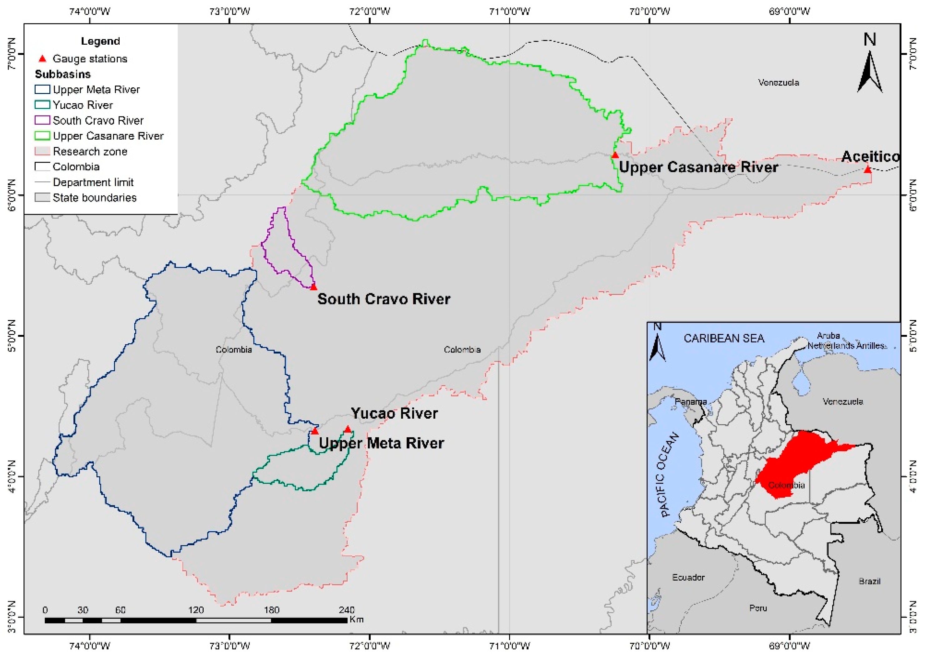
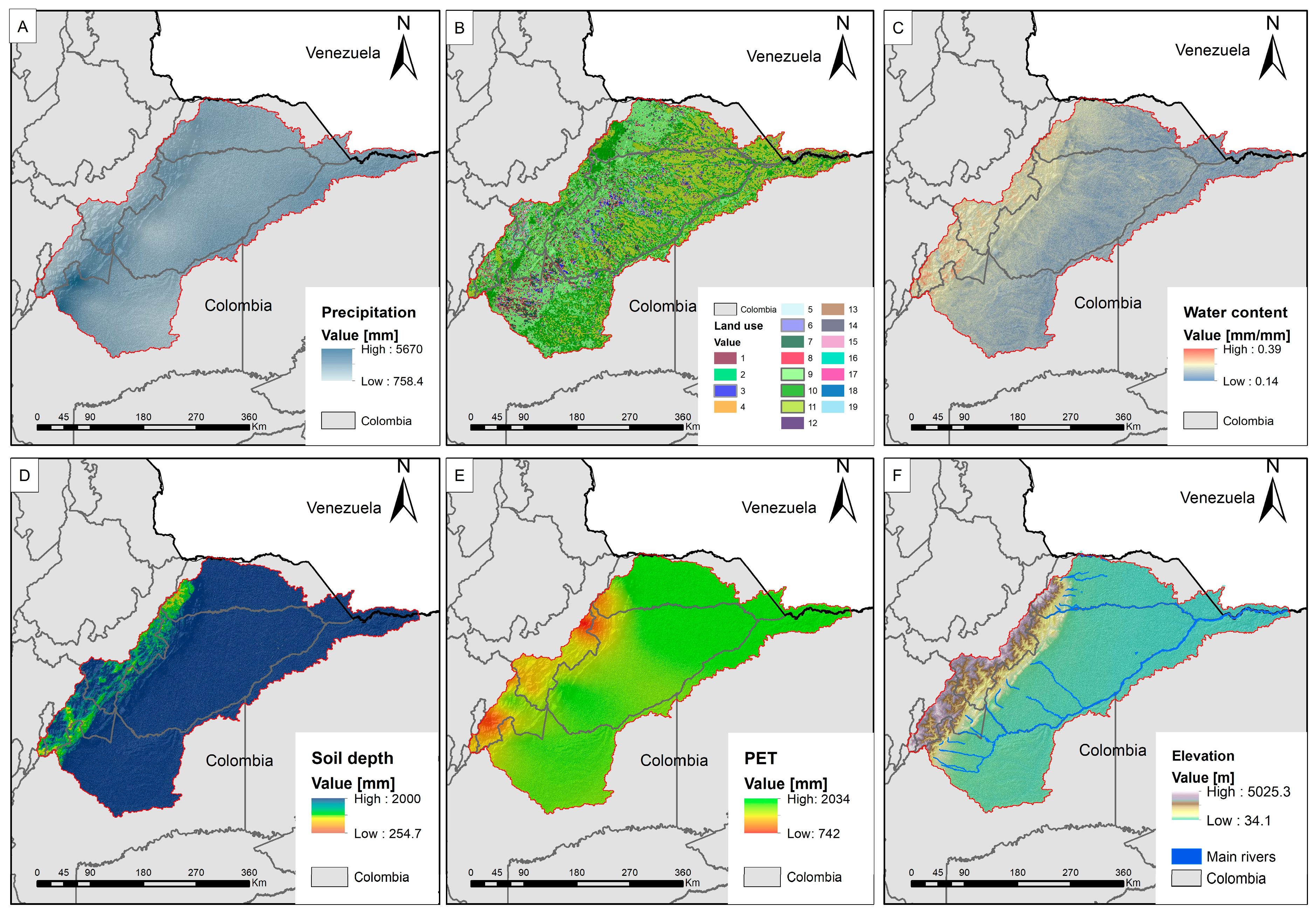
2.1. Study Area
2.2. Method
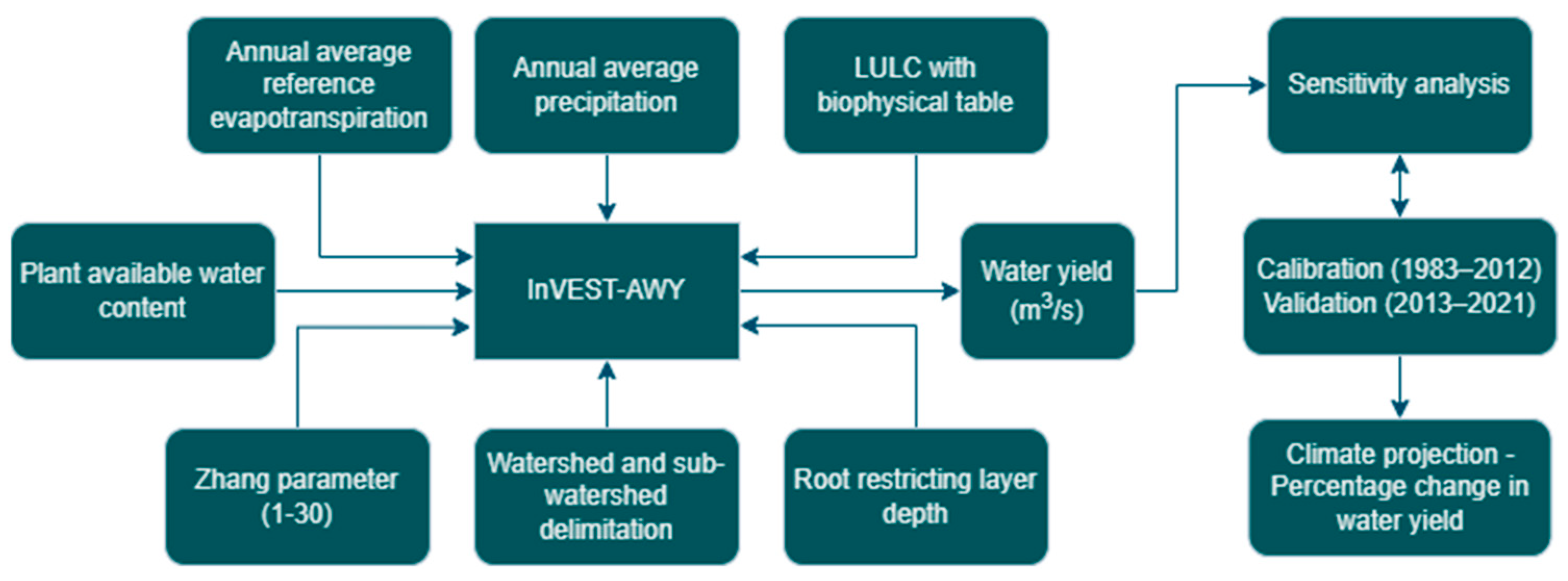
2.2.1. The InVEST–AWY Model
2.2.2. Data Requirements
2.2.3. Meteorological Data
2.2.4. Soil Data and Plant Available Water Content Data
2.2.5. Land-Use Data, Land-Cover Data, and Kc
2.2.6. River Water Discharge Data
2.2.7. Climate CMIP6 Scenarios
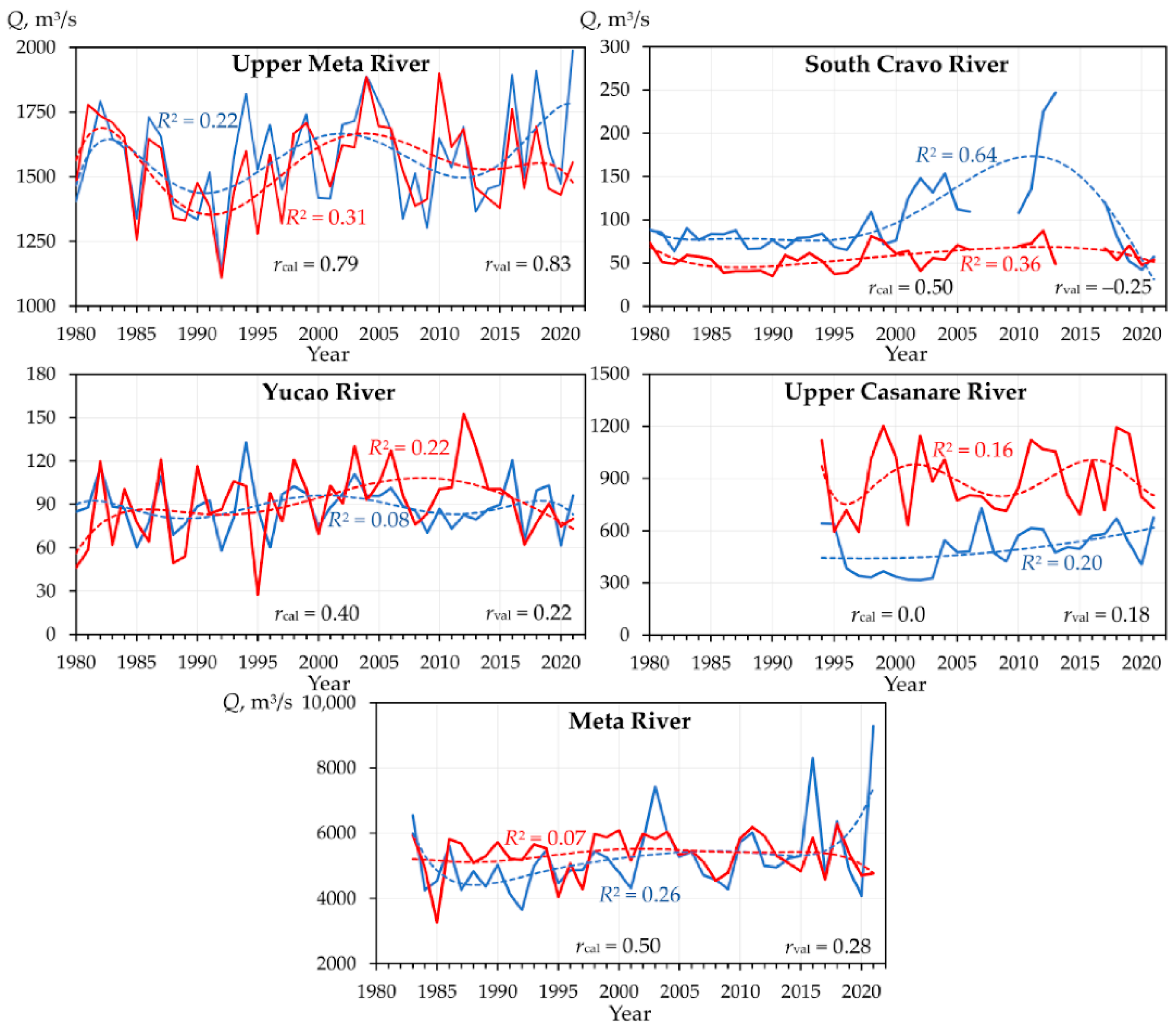
2.3. Calibration and Validation
3. Results
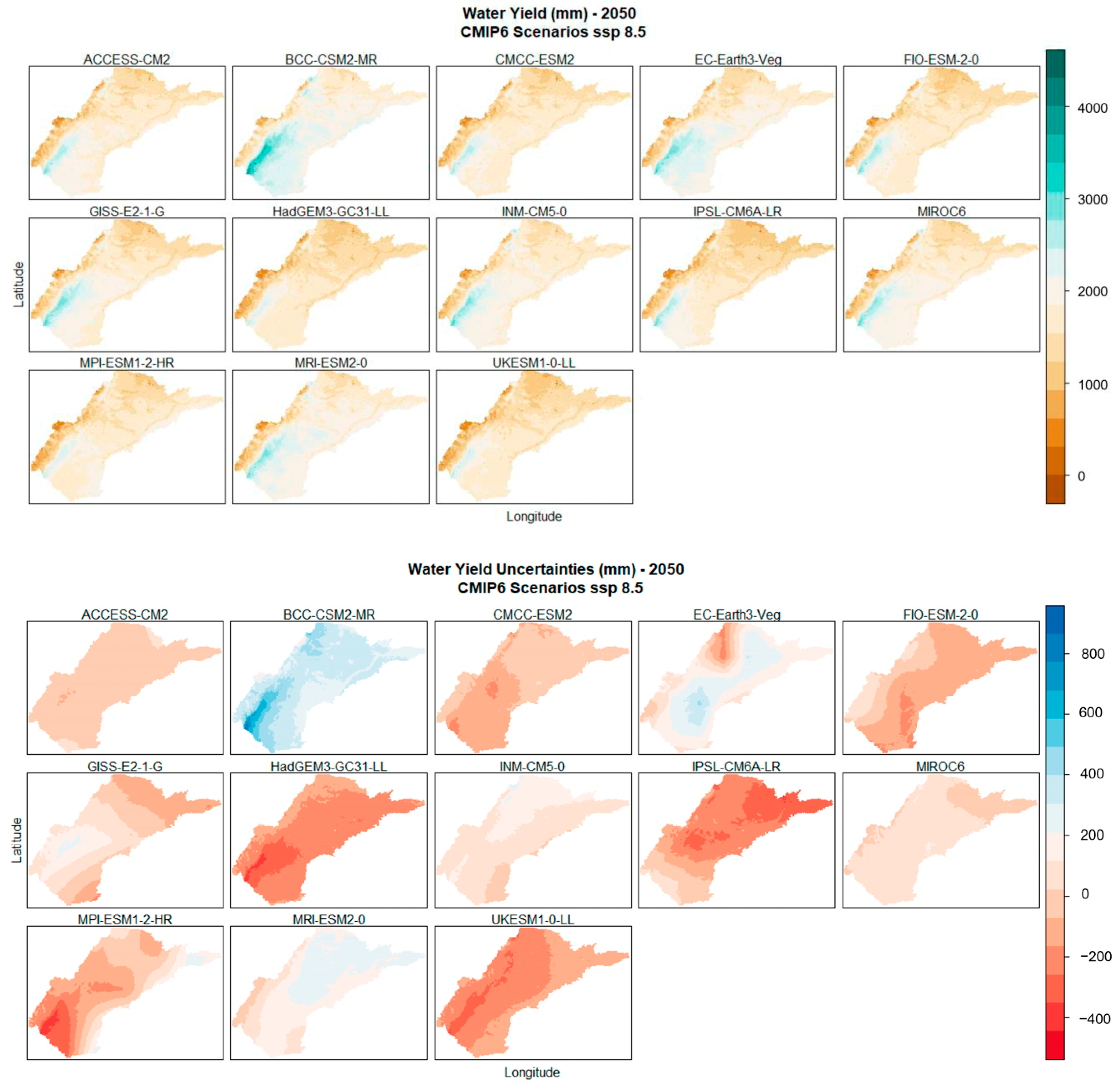
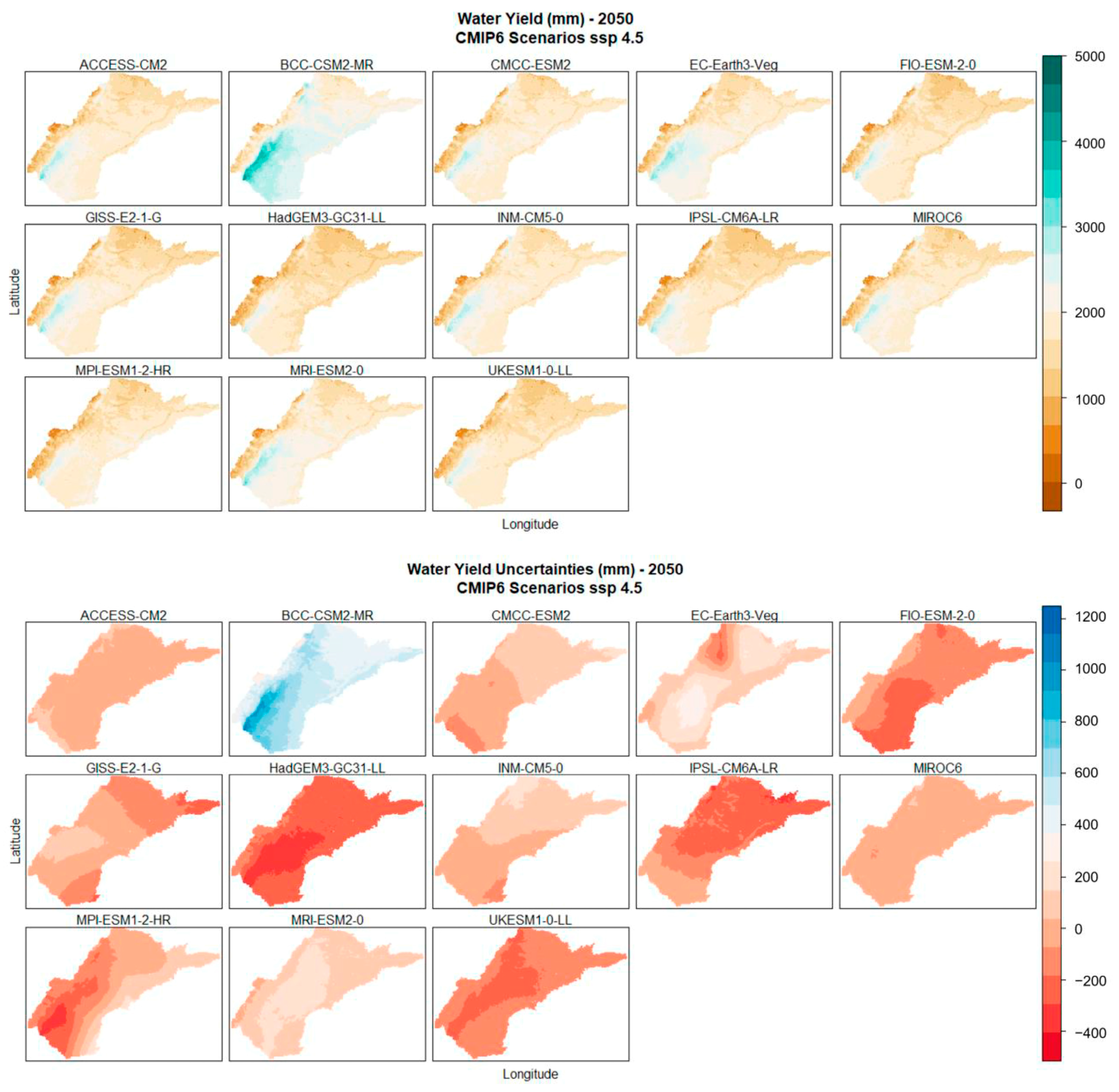
3.1. Changes in the Annual Water Yield Predicted 2050 under CMIP6 Scenarios
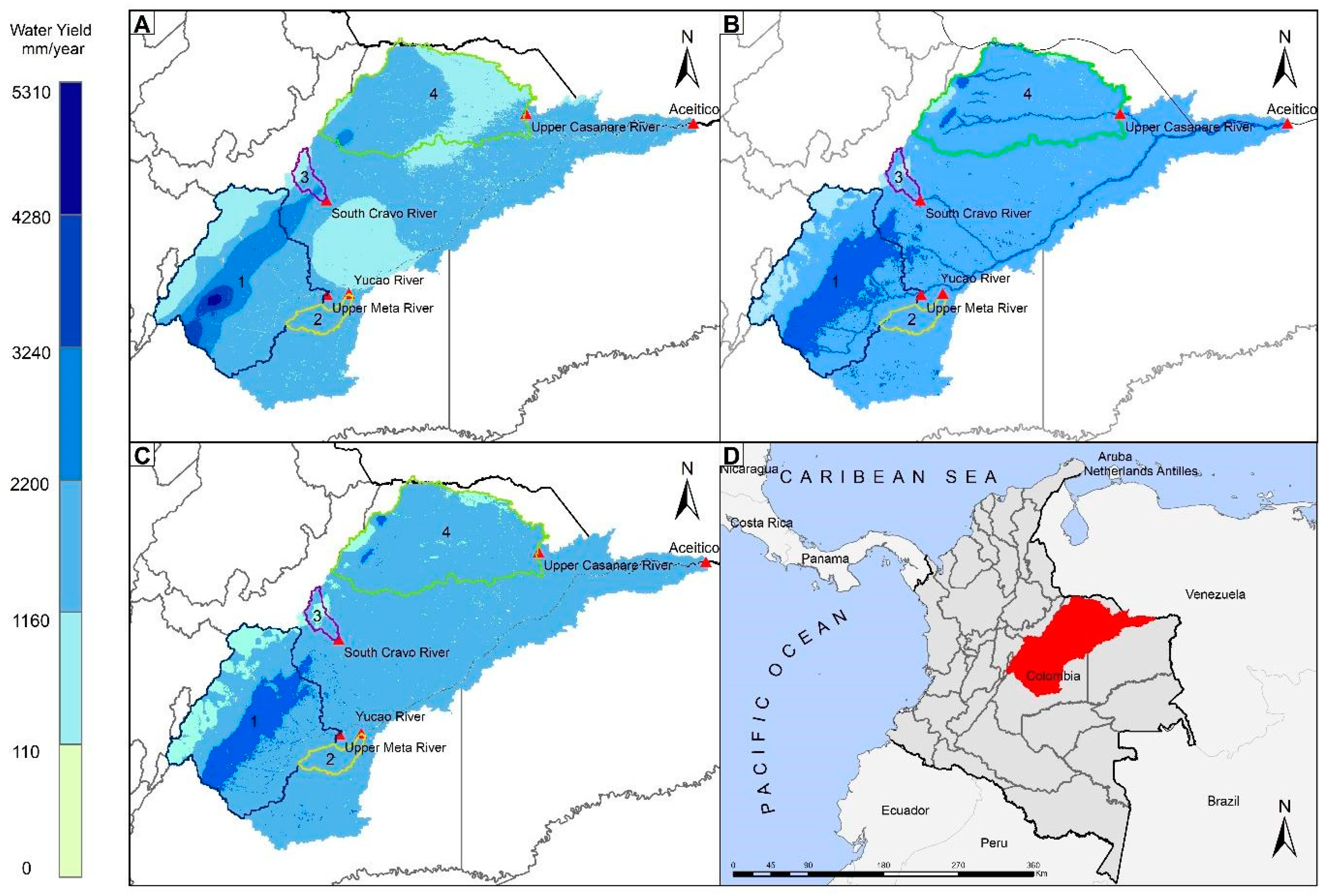
3.2. Spatial Variation in Water Yield for 1983–2012 and 2050 under Two Scenarios
4. Discussion
4.1. Model Limitations
4.2. Uncertainties in the Reported Information
4.3. Climate Change Uncertainties
5. Conclusions
- (1)
- For the Meta River basin, we predict a significant increase in simulated water flow from the current 5141.6 m3/s to 6397.5 m3/s by 2050 under the SSP 4.5 scenario, and an increase to 6101.5 m3/s under the SSP 8.5 scenario. This correlates with an increase in water yield by 24% and 19%, respectively, under the two future scenarios evaluated. The upper Meta River subbasin shows a slight decrease in water flow from the current 1600.6 m3/s to 1578.3 m3/s (SSP 4.5) and a decrease to 1511.3 m3/s (SSP 8.5), with water yield changes ranging by −1% and −6%, respectively. The upper Casanare River subbasin is expected to see a moderate rise in water yield from 976.3 m3/s to 1119.7 m3/s and 1059.9 m3/s under the SSP 4.5 and SSP 8.5 scenarios, respectively, with water yield changes rising by 19% and 9%, respectively. The Yucao River subbasin shows an increase from 95.9 m3/s to 113.3 m3/s and 109 m3/s, with water yield changes increasing by 18% and 15%, respectively. In contrast, the South Cravo River subbasin is predicted to face a decrease in water flow from the current 58.5 m3/s to 52.9 m3/s and 50.3 m3/s, with a significant drop in water yield changes of −10% and −14%, respectively, indicating a marked reduction in water availability.
- (2)
- Although the InVEST–AWY model provided acceptable results for the entire Meta River basin using data from 1983 to 2012, our study showed that the model is capable of effectively predicting potential impacts in well-calibrated areas, especially in the upper Meta River subbasin as defined by the Humapo gauging station.
- (3)
- The uncertainties observed in the thirteen global climate models according to SSP 4.5 and 8.5 scenarios stem from the varying predictions of increased water yield availability in the flatter regions of the main basin. This potential increase could lead to a higher likelihood of concurrent floods or river overflows, emphasizing the need for adaptation strategies in these areas.
- (4)
- Future research should prioritize two key areas. First, flood risk analysis and strategies are needed in areas that have potential for increased water yield, considering expected increases in water levels and the possibility of flooding. This area of research will include the use of models to predict floods, assess impacts on infrastructure and communities, and develop flood mitigation strategies. Second, it is important to study the socioeconomic impacts of water yield fluctuations, especially in regions facing declining water availability, such as the South Cravo River subbasin. Research in this area may focus on water management, impacts on agricultural practices, and impacts on community livelihoods.
- (5)
- Finally, it would be useful to carry out comparative studies using a range of both non-robust and robust hydrological models. This approach would serve to validate the study’s findings and provide a clearer understanding of the comparative advantages of various hydrological models, especially in regions with complex topography and scarce meteorological monitoring data in Colombia.
Author Contributions
Funding
Data Availability Statement
Acknowledgments
Conflicts of Interest
References
- IPCC. Impacts, Adaptation, and Vulnerability: Part A: Global and Sectoral Aspects; Cambridge University Press: Cambridge, UK, 2014. [Google Scholar]
- Bates, B.C.; Kundzewicz, Z.W.; Wu, S.; Palutikof, J.P. Climate Change and Water; Technical Paper of the Intergovernmental Panel on Climate Change; IPCC Secretariat: Geneva, Switzerland, 2008; p. 210. [Google Scholar]
- Vörösmarty, C.J.; McIntyre, P.B.; Gessner, M.O.; Dudgeon, D.; Prusevich, A.; Green, P.; Glidden, S.; Bunn, S.E.; Sullivan, C.A.; Liermann, C.R.; et al. Global Threats to Human Water Security and River Biodiversity. Nature 2010, 467, 555–561. [Google Scholar] [CrossRef] [PubMed]
- Dai, A. Increasing Drought under Global Warming in Observations and Models. Nat. Clim. Chang. 2013, 3, 52–58. [Google Scholar] [CrossRef]
- Budyko, M.I. Climate and Life; Academic Press: Cambridge, MA, USA, 1974. [Google Scholar]
- Hengade, N.; Eldho, T.I. Assessment of LULC and Climate Change on the Hydrology of Ashti Catchment, India Using VIC Model. J. Earth Syst. Sci. 2016, 125, 1623–1634. [Google Scholar] [CrossRef]
- Golmohammadi, G.; Rudra, R.; Prasher, S.; Madani, A.; Mohammadi, K.; Goel, P.; Daggupatti, P. Water Budget in a Tile Drained Watershed under Future Climate Change Using SWATDRAIN Model. Climate 2017, 5, 39. [Google Scholar] [CrossRef]
- Liu, L.; Xu, Z.; Huang, J. Impact of Climate Change on Streamflow in the Xitiaoxi Catchment, Taihu Basin. Wuhan Univ. J. Nat. Sci. 2009, 14, 525–531. [Google Scholar] [CrossRef]
- Valencia, J.B.; Guryanov, V.V.; Mesa-Diez, J.; Tapasco, J.; Gusarov, A.V. Assessing the Effectiveness of the Use of the InVEST Annual Water Yield Model for the Rivers of Colombia: A Case Study of the Meta River Basin. Water 2023, 15, 1617. [Google Scholar] [CrossRef]
- Abdullah, S.M.F.; Ahmed, S.I.; Hussain, E.; Hasan, F.; Ahmed, S. Drought Assessment of a Data-Scarced Watershed—Quetta Valley, Pakistan. Jordan J. Civ. Eng. 2023, 17, 310–321. [Google Scholar] [CrossRef]
- Kim, K.B.; Kwon, H.-H.; Han, D. Hydrological Modelling under Climate Change Considering Nonstationarity and Seasonal Effects. Hydrol. Res. 2015, 47, 260–273. [Google Scholar] [CrossRef]
- Bejagam, V.; Keesara, V.R.; Sridhar, V. Impacts of Climate Change on Water Provisional Services in Tungabhadra Basin Using InVEST Model. River Res. Appl. 2022, 38, 94–106. [Google Scholar] [CrossRef]
- Ryan, W.B.F.; Carbotte, S.M.; Coplan, J.O.; O’Hara, S.; Melkonian, A.; Arko, R.; Weissel, R.A.; Ferrini, V.; Goodwillie, A.; Nitsche, F.; et al. Global Multi-Resolution Topography Synthesis. Geochem. Geophys. Geosystems 2009, 10, Q03014. [Google Scholar] [CrossRef]
- Correa, H.D.; Ruíz, S.L.; Arevalo, L.M. Plan de Acción En Biodiversidad de La Cuenca Del Orinoco 2005–2015: Propuesta Técnica; Instituto de Investigación de Recursos Biológicos Alexander von Humboldt: Bogotá, Colombia, 2006; ISBN 978-958-8151-66-3. [Google Scholar]
- Hoz, J.V.D.L. Geografía económica de la Orinoquia. In Documentos de Trabajo sobre Economía Regional; Banco de la República: Bogotá, Colombia, 2009. [Google Scholar]
- CIAT Cormacarena. Plan Regional Integral de Cambio Cilmático para la Orinoquía (PRICCO); CIAT Publicación No 438; CIAT: Cali, Colombia, 2018; ISBN 978-958-694-168-6. [Google Scholar]
- NaturalCapitalProject Seasonal Water Yield—InVEST 3.6.0 Documentation. Available online: http://data.naturalcapitalproject.org/nightly-build/invest-users-guide/html/seasonal_water_yield.html (accessed on 4 May 2020).
- Yang, Y.; Donohue, R.J.; McVicar, T.R. Global Estimation of Effective Plant Rooting Depth: Implications for Hydrological Modeling. Water Resour. Res. 2016, 52, 8260–8276. [Google Scholar] [CrossRef]
- Hengl, T.; de Jesus, J.M.; Heuvelink, G.B.M.; Gonzalez, M.R.; Kilibarda, M.; Blagotić, A.; Shangguan, W.; Wright, M.N.; Geng, X.; Bauer-Marschallinger, B.; et al. SoilGrids250m: Global Gridded Soil Information Based on Machine Learning. PLoS ONE 2017, 12, e0169748. [Google Scholar] [CrossRef] [PubMed]
- IDEAM Consulta y Descarga de Datos Hidrometeorológicos. Available online: http://dhime.ideam.gov.co/atencionciudadano/ (accessed on 19 February 2023).
- R: Extraterrestrial Solar Radiation. Available online: https://search.r-project.org/CRAN/refmans/envirem/html/ETsolradRasters.html (accessed on 19 February 2023).
- IDEAM. Mapas de Suelos del Territorio Colombiano a Escala 1:100.000; IDEAM: Bogotá, Colombia, 2018.
- Fick, S.E.; Hijmans, R.J. WorldClim 2: New 1-Km Spatial Resolution Climate Surfaces for Global Land Areas. Int. J. Climatol. 2017, 37, 4302–4315. [Google Scholar] [CrossRef]
- Navarro-Racines, C.; Tarapues, J.; Thornton, P.; Jarvis, A.; Ramirez-Villegas, J. High-Resolution and Bias-Corrected CMIP5 Projections for Climate Change Impact Assessments. Sci. Data 2020, 7, 7. [Google Scholar] [CrossRef] [PubMed]
- Pimentel, J.N.; Rogéliz Prada, C.A.; Walschburger, T. Hydrological Modeling for Multifunctional Landscape Planning in the Orinoquia Region of Colombia. Front. Environ. Sci. 2021, 9, 673215. [Google Scholar] [CrossRef]
- Yu, Y.; Sun, X.; Wang, J.; Zhang, J. Using InVEST to Evaluate Water Yield Services in Shangri-La, Northwestern Yunnan, China. PeerJ 2022, 10, e12804. [Google Scholar] [CrossRef] [PubMed]
- Yang, D.; Liu, W.; Tang, L.; Chen, L.; Li, X.; Xu, X. Estimation of Water Provision Service for Monsoon Catchments of South China: Applicability of the InVEST Model. Landsc. Urban Plan. 2019, 182, 133–143. [Google Scholar] [CrossRef]
- Redhead, J.W.; Stratford, C.; Sharps, K.; Jones, L.; Ziv, G.; Clarke, D.; Oliver, T.H.; Bullock, J.M. Empirical Validation of the InVEST Water Yield Ecosystem Service Model at a National Scale. Sci. Total Environ. 2016, 569–570, 1418–1426. [Google Scholar] [CrossRef] [PubMed]
- Benavides Guerrero, C.E.; Caro Caro, L.E.; Mariño Martínez, J.E. Determination of the Hydraulic Behavior of Aquifers in Northern Orinoquia, Colombia. Cienc. E Ing. Neogranadina 2021, 31, 109–126. [Google Scholar] [CrossRef]


| Data | Period | Source | Tool | Format |
|---|---|---|---|---|
| Annual average precipitation | 1983–2021 | Instituto de Hidrología, Meteorología y Estudios Ambientales—IDEAM | R version 4.1.2 | Raster |
| 2040–2060 | Worldclim—CMIP6 scenarios | |||
| Annual average water discharge | 1983–2021 | Instituto de Hidrología, Meteorología y Estudios Ambientales—IDEAM | – | CSV |
| Evapotranspiration | 1983–2021 | Instituto de Hidrología, Meteorología y Estudios Ambientales IDEAM (air temperature) | Hargreaves equation | Raster |
| 2040–2060 | Worldclim—CMIP6 scenarios (air temperature) | |||
| Root restricting layer depth | – | [18] | R version 4.1.2 | Raster |
| Plant available water content | – | [19] | R version 4.1.2 | Raster |
| Land-use/Land-cover | 2018 | Instituto de Hidrología, Meteorología y Estudios Ambientales—IDEAM | ArcMAP software 10.6 | Raster |
| Watersheds DEM | – | GMRTMapTool/ArcSWAT | ArcMAP software 10.6 | Shapefile |
| Biophysical table | – | FAO/IDEAM data | – | CSV |
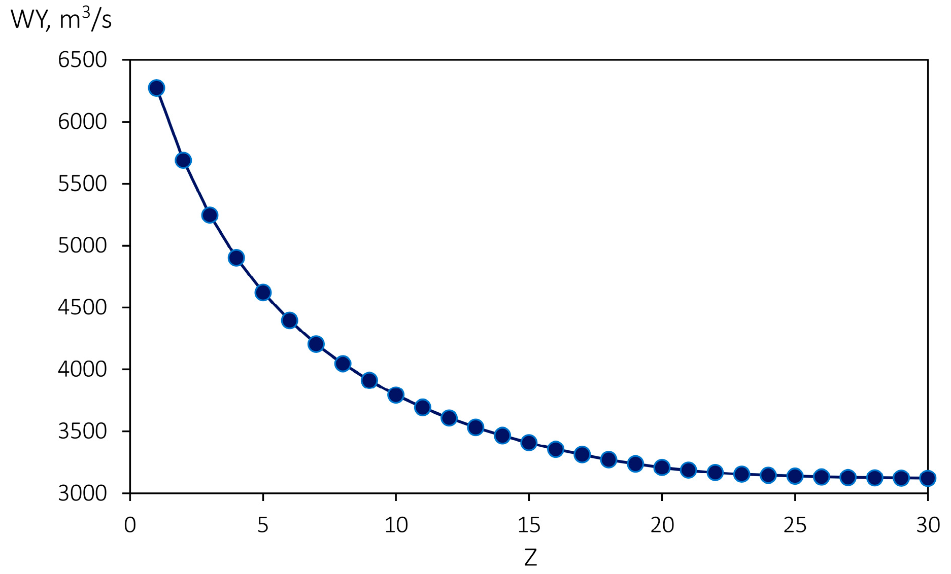
| Z coefficient | – | – | – | Ranges from 1 to 30 |
| LU Code | LULC Description | Kc |
|---|---|---|
| 3 | Cereals | 1.2 |
| 4 | Oilseeds and legumes | 1.2 |
| 8 | Agroforestry crops | 1.2 |
| 2 | Short duration crops | 1.1 |
| 7 | Permanent crops | 1.1 |
| 12 | Shrubland | 1.1 |
| 13 | Secondary vegetation | 1.1 |
| 9 | Pasture | 1.0 |
| 10 | Forest | 1.0 |
| 18 | Aquatic vegetation | 1.0 |
| 19 | Water surface | 1.0 |
| 5 | Vegetables | 0.9 |
| 6 | Tubers | 0.9 |
| 11 | Grassland | 0.9 |
| 14 | Sand | 0.3 |
| 15 | Rocks | 0.3 |
| 16 | Bare soils/grounds | 0.3 |
| 17 | Snow cover | 0.2 |
| 1 | Urban area | 0.1 |
| Code | Station (River) | Basin Area (km2) | Automatic | Period | AAWD (m3/s) |
|---|---|---|---|---|---|
| 35117010 | Humapo (upper Meta River) | 26,343 | No | 1980–2021 | 1576.3 |
| 35127020 | Campamento Yucao (Yucao River) | 1797 | No | 1980–2021 | 88.3 |
| 35217010 | Puente Yopal (South Cravo River) | 1187 | Yes | 1980–2021 | 97.2 |
| 36027050 | Cravo Norte (upper Casanare River) | 22,872 | No | 1994–2021 | 494.2 |
| 35257040 | Aceitico (Meta River) | 113,981 | No | 1983–2021 | 5256.8 |
| 2050 Shared Socioeconomic Pathways Scenario 4.5 | ||||||||
|---|---|---|---|---|---|---|---|---|
| Model | Precipitation, mm | Evapotranspiration (Eto), mm | ||||||
| Max | Min | Mean | SD | Max | Min | Mean | SD | |
| ACCESS-CM2 | 4236.4 | 898.6 | 2537.1 | 420.2 | 1850.8 | 675.8 | 1710.1 | 195.8 |
| BCC-CSM2-MR | 5293.1 | 1109.4 | 3115.3 | 548.1 | 1870.4 | 688.8 | 1733.1 | 191.5 |
| CMCC-ESM2 | 3921.5 | 905.1 | 2572.1 | 405.3 | 1853.4 | 673.1 | 1708.7 | 197.5 |
| EC-Earth3-Veg | 4191.3 | 887.5 | 2659.4 | 476.2 | 1832.4 | 655.8 | 1668.6 | 186.5 |
| FIO-ESM-2-0 | 3916.8 | 879.5 | 2385.4 | 393.5 | 1880.6 | 681.6 | 1737.6 | 203.0 |
| GISS-E2-1-G | 4105.0 | 868.9 | 2478.1 | 448.2 | 1844.7 | 668.7 | 1705.2 | 198.6 |
| HadGEM3-GC31-LL | 3710.0 | 811.5 | 2291.2 | 381.6 | 1937.2 | 729.7 | 1775.5 | 207.4 |
| INM-CM5-0 | 4085.9 | 939.5 | 2572.7 | 406.6 | 1801.9 | 637.0 | 1664.0 | 192.8 |
| IPSL-CM6A-LR | 4150.8 | 802.0 | 2356.7 | 446.3 | 1856.2 | 678.0 | 1701.1 | 193.6 |
| MIROC6 | 4018.7 | 885.1 | 2508.5 | 423.3 | 1823.0 | 642.7 | 1678.2 | 202.8 |
| MPI-ESM1-2-HR | 3728.4 | 827.7 | 2462.2 | 412.1 | 1813.1 | 655.1 | 1659.1 | 185.3 |
| MRI-ESM2-0 | 4246.1 | 913.7 | 2665.6 | 454.7 | 1814.9 | 636.4 | 1663.0 | 193.5 |
| UKESM1-0-LL | 3850.5 | 814.3 | 2381.2 | 405.6 | 1915.2 | 721.8 | 1750.9 | 198.0 |
| 2050 Shared Socioeconomic Pathways Scenario 8.5 | ||||||||
|---|---|---|---|---|---|---|---|---|
| Model | Precipitation, mm | Evapotranspiration (Eto), mm | ||||||
| Max | Min | Mean | SD | Max | Min | Mean | SD | |
| ACCESS-CM2 | 4003.2 | 845.7 | 2438.1 | 411.2 | 1885.3 | 700.9 | 1741.6 | 197.5 |
| BCC-CSM2-MR | 4904.6 | 1005.1 | 2837.5 | 477.1 | 1906.2 | 720.5 | 1761.7 | 189.7 |
| CMCC-ESM2 | 3765.6 | 820.1 | 2382.2 | 390.3 | 1875.8 | 693.0 | 1730.2 | 197.6 |
| EC-Earth3-Veg | 4111.6 | 892.3 | 2615.8 | 468.0 | 1868.7 | 671.4 | 1692.0 | 187.5 |
| FIO-ESM-2-0 | 3935.1 | 883.1 | 2371.7 | 395.0 | 1909.8 | 699.8 | 1764.8 | 205.9 |
| GISS-E2-1-G | 4147.1 | 863.8 | 2471.8 | 458.3 | 1865.2 | 681.1 | 1723.2 | 200.0 |
| HadGEM3-GC31-LL | 3596.7 | 807.2 | 2255.3 | 374.8 | 1968.2 | 752.4 | 1805.9 | 209.2 |
| INM-CM5-0 | 4141.2 | 910.3 | 2539.5 | 414.2 | 1810.3 | 646.2 | 1672.2 | 191.2 |
| IPSL-CM6A-LR | 4100.2 | 784.3 | 2263.3 | 444.6 | 1889.1 | 701.7 | 1730.2 | 195.1 |
| MIROC6 | 4071.5 | 872.9 | 2505.1 | 435.9 | 1844.0 | 646.5 | 1693.3 | 205.7 |
| MPI-ESM1-2-HR | 3533.9 | 829.3 | 2367.6 | 393.3 | 1857.3 | 684.7 | 1700.4 | 186.6 |
| MRI-ESM2-0 | 4068.2 | 893.3 | 2628.0 | 437.1 | 1846.2 | 652.8 | 1686.2 | 193.5 |
| UKESM1-0-LL | 3635.6 | 770.3 | 2283.6 | 395.4 | 1992.6 | 777.7 | 1814.8 | 205.2 |
| Basin/Subbasin | NSE | RMSE | rcal | rval | DIF STD |
|---|---|---|---|---|---|
| Meta River | 0.07 | 1071.61 | 0.5 | 0.28 | 1083.62 |
| Upper Meta River | 0.49 | 135.37 | 0.79 | 0.83 | 132.81 |
| Yucao River | 0.03 | 57.49 | 0.4 | 0.22 | 40.61 |
| South Cravo River | −1.29 | 24.75 | 0.5 | −0.25 | 24.92 |
| Upper Casanare River | −0.49 | 452.32 | 0 | 0.18 | 261.12 |
| Station ID | Basin/Subbasin | Climate Scenario | Precipitation (mm) | PET (mm) | AET (mm) | Water Yield Volume (m3) | Simulated Water Flow (m3/s) | Measured Mean Flow for 1983–2012 (m3/s) | Water Yield Changes (%) |
|---|---|---|---|---|---|---|---|---|---|
| 35257040 | Meta River basin | Current | 2255.3 | 1672.0 | 726.1 | 1.73 × 10¹¹ | 5141.6 | 5063.84 | 2 1 |
| 2050 SSP 4.5 | 2553.8 | 1776.8 | 773.9 | 2.02 × 10¹¹ | 6397.5 | 24 | |||
| 2050 SSP 8.5 | 2474.2 | 1805.8 | 776.7 | 1.92 × 10¹¹ | 6101.5 | 19 | |||
| 35117010 | Upper Meta River subbasin | Current | 2683.9 | 1732.2 | 769.8 | 5.05 × 10¹⁰ | 1600.6 | 1559 | 3 1 |
| 2050 SSP 4.5 | 2647.9 | 1676.3 | 760.5 | 4.98 × 10¹⁰ | 1578.3 | −1 | |||
| 2050 SSP 8.5 | 2571.8 | 1705.3 | 764.5 | 4.77 × 10¹⁰ | 1511.3 | −6 | |||
| 36027050 | Upper Casanare River subbasin | Current | 2011.6 | 1469.4 | 666.0 | 3.08 × 10¹⁰ | 976.3 | 470 | 108 1 |
| 2050 SSP 4.5 | 2307.3 | 1783.5 | 764.5 | 3.53 × 10¹⁰ | 1119.7 | 15 | |||
| 2050 SSP 8.5 | 2226.9 | 1813.3 | 766.5 | 3.34 × 10¹⁰ | 1059.9 | 9 | |||
| 35127020 | Yucao River subbasin | Current | 2504.5 | 2039.2 | 821.2 | 3.02 × 10⁹ | 95.9 | 82.7 | 16 1 |
| 2050 SSP 4.5 | 2804.1 | 1934.3 | 815.4 | 3.57 × 10⁹ | 113.3 | 18 | |||
| 2050 SSP 8.5 | 2732.2 | 1964.8 | 818.6 | 3.44 × 10⁹ | 109.0 | 14 | |||
| 35217010 | South Cravo River subbasin | Current | 2238.6 | 1498.0 | 690.4 | 1.85 × 10⁹ | 58.5 | 98.7 | −41 1 |
| 2050 SSP 4.5 | 2086.3 | 1493.7 | 684.5 | 1.67 × 10⁹ | 52.9 | −10 | |||
| 2050 SSP 8.5 | 2021.8 | 1522.6 | 688.6 | 1.59 × 10⁹ | 50.3 | −14 |
Disclaimer/Publisher’s Note: The statements, opinions and data contained in all publications are solely those of the individual author(s) and contributor(s) and not of MDPI and/or the editor(s). MDPI and/or the editor(s) disclaim responsibility for any injury to people or property resulting from any ideas, methods, instructions or products referred to in the content. |
© 2024 by the authors. Licensee MDPI, Basel, Switzerland. This article is an open access article distributed under the terms and conditions of the Creative Commons Attribution (CC BY) license (https://creativecommons.org/licenses/by/4.0/).
Share and Cite
Valencia, J.B.; Guryanov, V.V.; Mesa-Diez, J.; Diaz, N.; Escobar-Carbonari, D.; Gusarov, A.V. Predictive Assessment of Climate Change Impact on Water Yield in the Meta River Basin, Colombia: An InVEST Model Application. Hydrology 2024, 11, 25. https://doi.org/10.3390/hydrology11020025
Valencia JB, Guryanov VV, Mesa-Diez J, Diaz N, Escobar-Carbonari D, Gusarov AV. Predictive Assessment of Climate Change Impact on Water Yield in the Meta River Basin, Colombia: An InVEST Model Application. Hydrology. 2024; 11(2):25. https://doi.org/10.3390/hydrology11020025
Chicago/Turabian StyleValencia, Jhon B., Vladimir V. Guryanov, Jeison Mesa-Diez, Nilton Diaz, Daniel Escobar-Carbonari, and Artyom V. Gusarov. 2024. "Predictive Assessment of Climate Change Impact on Water Yield in the Meta River Basin, Colombia: An InVEST Model Application" Hydrology 11, no. 2: 25. https://doi.org/10.3390/hydrology11020025
APA StyleValencia, J. B., Guryanov, V. V., Mesa-Diez, J., Diaz, N., Escobar-Carbonari, D., & Gusarov, A. V. (2024). Predictive Assessment of Climate Change Impact on Water Yield in the Meta River Basin, Colombia: An InVEST Model Application. Hydrology, 11(2), 25. https://doi.org/10.3390/hydrology11020025