Abstract
The vadose zone acts as a natural buffer against groundwater contamination, and thus, its attenuation capacity (AC) directly affects groundwater vulnerability to pollutants. A regression model from the previous study predicting the overall AC of soils against diesel was further expanded to the GIS-based overlay-index model. Among the six physicochemical parameters used in the regression model, saturation degree (SD) is notably susceptible to climatological and meteorological events. To accommodate the lack of soil SD historical data, a series of infiltration simulations were separately conducted using Phydrus code with moving boundary conditions (i.e., rainfall records). The temporal variation of SD and the resulting AC under transient conditions are captured by building a space–time cube using a temporal raster across the study area within the designated time frame (1997–2022). The emerging hot spot analysis (EHSA) tool, based on the Getis–Ord Gi* and Mann–Kendall statistics, is applied to further identify any existing pattern associated with both SD and AC in both space and time simultaneously. Under stationary conditions, AC decreases along depth and is relatively lower near water bodies. Similarly, AC cold spot trends also show up near water bodies under transient conditions. The result captures not only the trends across time but also shows the exact location where the changes happen. The proposed framework provides an efficient tool to look for locations that have a persistently low or a gradually decreasing ability to attenuate diesel over time, indicating the need for stricter management regulations from a long-term perspective.
1. Introduction
Despite the numerous efforts [1,2,3] that have been taken to address the fate of various contaminants in the vadose zone, it is still inadequate to achieve a better understanding of natural attenuation therein due to the non-stationary nature. Process-based models (e.g., HYDRUS) are available for estimating the contaminant migration to the groundwater through a vadose zone, which solves Richard’s equation to estimate the water flow under unsaturated conditions with accompanying contaminant transport [4]. However, it is difficult to extend their application to a large scale due to the heterogeneity in the subsurface properties and the computational cost. On the other hand, the GIS-based spatial model is suitable for large-scale estimation and has been often used for groundwater vulnerability assessment. One of the most widely used models, DRASTIC [5] employs seven hydrogeological properties as the input parameters to assess the intrinsic groundwater vulnerability. Unfortunately, however, it failed to include the natural attenuation of contaminants in a vadose zone [6,7,8]. A previous study by Woo et al. (2022) addressed the effect of soil physicochemical properties on the overall attenuation capacity (AC) of a vadose zone soil against diesel, a type of refined petroleum product [9]. They found that six parameters consisting of two chemical properties and four physical properties, including soil moisture, play an essential role in soil’s natural AC against diesel. Based on multiple linear regression analyses, an empirical relationship between the soil properties and the diesel AC of a vadose zone was suggested. Among those factors, however, the soil moisture is susceptible to temporally varying climatological and meteorological events.
The first few centimeters of surface soils have been reported to be affected mostly by climate change due to the complex interaction between the atmosphere and lithosphere near the ground surface, especially in relation to soil moisture [10,11,12,13]. The previous studies also mentioned the seasonal effects of meteorological events on the soil. Moreover, climate change should affect meteorological phenomena and alter global precipitation patterns, and thus, assessing its effect on AC along with the potential SD shifts might give a new understanding of the groundwater vulnerability to the contamination. However, soil SD data are not readily available. One way to obtain the SD is to simulate the soil water content on the basis of the climatological and meteorological data and calculate the SD on the basis of the soil properties. In this study, the spatiotemporal distribution of diesel AC in the city of South Korea (Namyangju city) was estimated with a focus on the variation of SD upon meteorological and climatological events.
Another problem is capturing the changes in SD and AC over time and space. Temporal changes are usually compared with snapshots between time snaps, e.g., forest coverage [14]. While comparing different periods can be useful, it may not capture the nuances of changes that occur between those periods. These in-between trends may not be fully captured by the comparison. It also cannot show where the areas are experiencing more or less changes over time. The emerging hot spot analysis (EHSA) tool in ArcGIS, developed by ESRI, provided a robust statistical assessment that simultaneously gives back the spatial and temporal hot and cold spot trend [15]. Even though EHSA has been applied in disease outbreaks [16,17], accident occurrence [18], flooding and drought [19,20,21], forest loss [22], and conservation monitoring [23,24], its application in soil vulnerability especially on vadose zone AC has not been recorded. Therefore, incorporating EHSA into the vulnerability study will provide a new way to assess and understand the dynamics of soil SD, AC, or other general vulnerability assessments.
The SD profile was obtained from the numerical simulation with moving boundary conditions, and subsequently, EHSA was performed to capture the temporal trends of both SD and AC within the designated time frame (1997–2022). However, we would like to note that the results we are presenting in this paper are solely for illustrative purposes regarding how incorporating temporal data with EHSA can enhance our understanding of environmental vulnerability.
2. Materials and Methods
2.1. Empirical Equation for Diesel Attenuation Capacity
Woo et al. (2022) developed an empirical relationship for determining the diesel attenuation capacity of a vadose zone with several soil properties [9]. Through laboratory experimentation and regression analysis, six parameters were identified as key factors affecting the attenuation capacity of a vadose zone to degrade diesel contamination therein. These parameters include soil organic matter content (OM), total phosphorus (TP), coefficient of uniformity (Cu), van Genuchten’s n parameter (n), soil saturation degree (SD), and the soil particle size at which 30% of the material is finer (D30). The vadose zone attenuation capacity in this study was calculated using the equation below:
where the subscript R represents the rated value based on min–max data normalization followed by an evenly spaced binning of the data (Table 1). The OM in the soil is a significant factor that determines the biodegradation of organic contaminants such as diesel, which primarily consists of hydrophobic materials that can retain them as well; microbial growth and reproduction use those contaminants as a source of carbon and energy, leading to biodegradation of diesel in the soil [25]. Soils with higher OM have a greater capacity to retain and break down diesel. In addition, phosphorus is a crucial nutrient for microbial growth in soil, alongside carbon and nitrogen. Microorganisms use phosphorus to synthesize cellular components, such as nucleic acids [26].

Table 1.
Parameter rating classification ranges.
Soil grading is determined by the coefficient of uniformity (Cu), which is the ratio of D60 to D10. A higher Cu means that the soil is better graded, with a more even composition of particles of different sizes. A uniform soil sample has particles with similar dimensions, resulting in a surface area that may be larger or smaller depending on the governing particle size. D30, which represents the size of soil particles at which 30% of the soil (by weight) is finer than that size, supports the effect of soil particle size distribution on the overall AC. Soil with coarse particles and poor grading has a higher D30 value, which is closer to or within the range of sandy soil. Lower Cu paired with higher D30 indicates bigger pore sizes, which could promote the volatilization of diesel components. Bigger pores also provide less surface area for attachment and higher mobility for microbes to access substrates, electron donors/acceptors, and nutrients. D30 can therefore provide additional information about pore size and soil uniformity in the area under study.
A min–max data normalization was applied, as shown in Equation (2), and the normalized data were classified into five rating classes with equal intervals (Table 1). The minimum and maximum values used for each parameter were the global minimum and maximum values across the 100 cm soil depth at the area of interest considered in this study. The min–max values of each parameter can be found in the Supplementary Materials (Table S1).
All these processes were performed in R studio [16], and the outputs are temporal SD and AC raster files with a spatial resolution of 100 m × 100 m. These raster files were then used as inputs in ArcGIS [27] for building space–time cubes and running EHSA (Section 2.3).
2.2. Parameter Estimation and Ratings
This study used publicly available data for the parameter estimation and ratings. The Korean Rural Development Administration (RDA) provides soil maps as vector and gridded data, which include information on soil series, soil texture, parent materials, and more. The laboratory test data sheets, which show the soil physicochemical characteristics, like sand, silt, clay (SSC) distribution, soil organic carbon (SOC), bulk density, water content, and pH, are also provided. Table 2 summarizes the data used to create thematic layers in this study.
Table 2.
Thematic layers used for attenuation capacity analyses.
Soil organic matter (OM) content was calculated by multiplying soil organic carbon (SOC) content and the van Bemmelen factor (Equation (3)) [28]. This conversion assumes that 58% of OM is in the form of SOC [28,29].
OM = 1.724 × SOC
Total phosphorus in the soil was estimated on the basis of the relationship between TP and SOC described by Hou et al. (2018) for natural terrestrial ecosystems [30].
In the laboratory test data sheet published by Korea RDA, the particle size distribution of soil is divided into sand, silt, and clay. Sand is classified again as very fine, fine, medium, coarse, and very coarse. Silt and clay are divided again as fine and coarse. These subgroups are presented as the percent fraction of a particle size range. The particle size defining 10%, 30%, and 60% finer soil particles in a particle size distribution curve is represented as D10, D30, and D60, respectively. Since the data range is a continuous scale from finest to coarsest, interpolation is used to find the values of D10, D30, and D60. D30 is used directly in the attenuation capacity model, while D10 and D60 are part of uniformity estimation. The uniformity coefficient is a measure representing how well the soil is graded and can be obtained by the ratio of D60 to D10 (Equation (4)).
Rosetta is a software that adopts a hierarchical pedotransfer function (PTF), which allows the estimation of water retention parameters, including van Genuchten’s (VG’s) n [31,32,33]. HYDRUS-1D (Ver. 4.20) is a popular numerical simulator used in the field of soil physics that incorporated a simplified version of Rosetta in its module [34]. This study used Rosetta PTF in HYDRUS-1D to estimate the VG’s n on the basis of the sand, silt, and clay content for each soil series. The usage of only SSC distribution for n estimation was mainly due to data limitations regarding bulk density and water content (soil field moisture), which were not available for the entire soil series.
2.3. Estimation of Temporal Changes in Soil Moisture and Resulting AC
In order to capture the temporal variation of the attenuation capacity according to the saturation degree, an infiltration simulation was conducted to obtain water content profiles using a Python-based HYDRUS-1D module, Phydrus [35], under moving boundary conditions. Historical meteorological data in the model city for 26 years (1997–2022) were obtained from the KMA (Korea Meteorological Administration) (Figure S1). The input data for the simulation included precipitation, atmospheric temperature, and soil profile (lithology and thickness). The outputs were the daily water content data at ten different depths (each 10 cm intervals along 100 cm depth) for the 46-soil series considered in the study (Figure S2). SD can be calculated from soil water contents as follows (Equation (5)):
where represents water content and and are the residual and saturated water contents, respectively. Upon the completion of the SD series, the temporal AC was then calculated using Equation (1), and raster files were built using R based on the SD data that were prepared. In this study, we focus on seasonal trends; thus the output raster is the averaged seasonal value of AC and SD for each year during the period 1997–2022.
2.4. Emerging Hot Spot Analysis
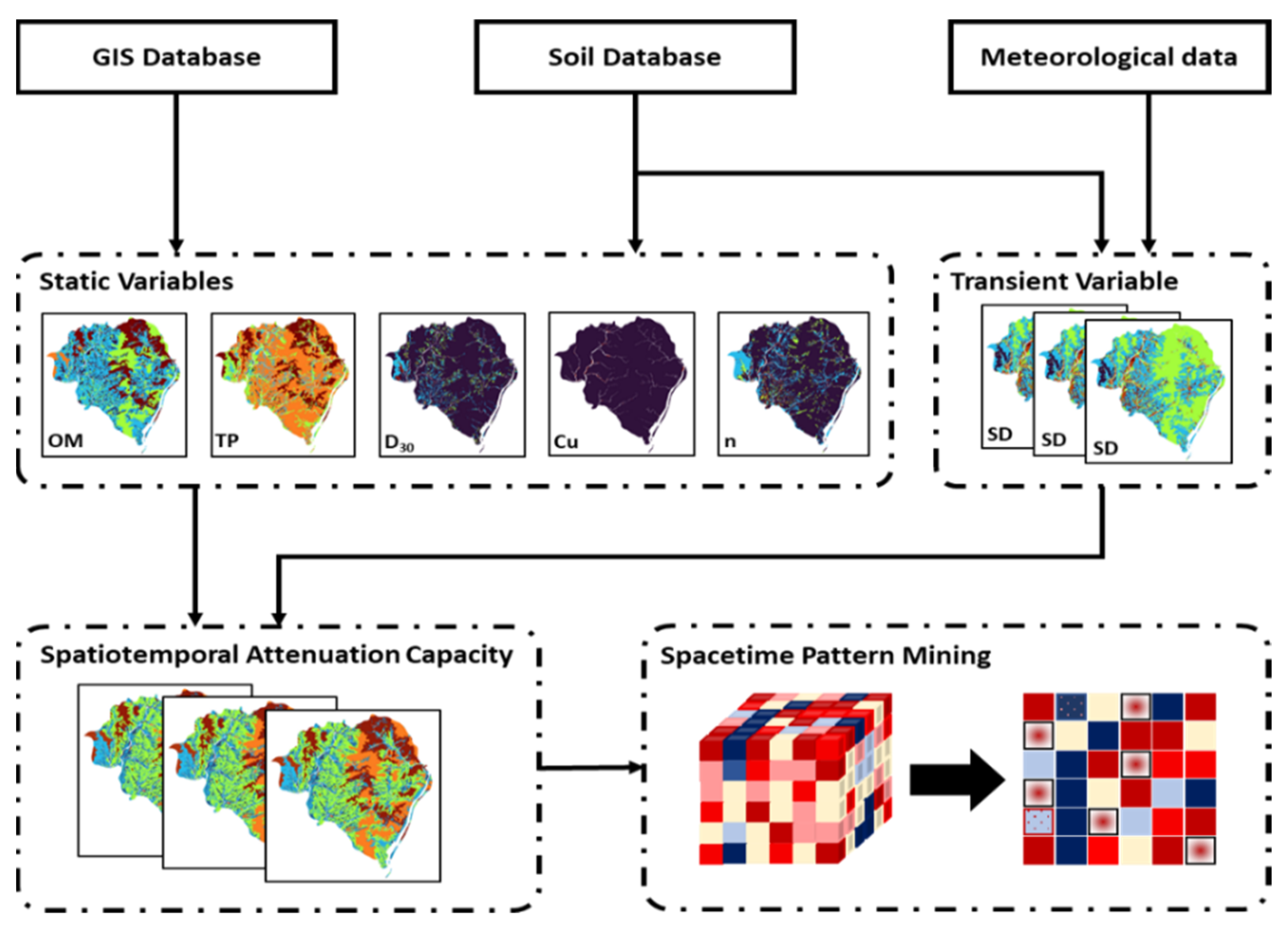
The process started with building space–time cubes (STCs), 3D visualizations of a geographical phenomenon. The horizontal plane of the cube represents the spatial context of the data (longitude and latitude), while the vertical axis represents time [17]. Each data point is treated as a bin and contains the attenuation capacity information for an exact location at a specific time. A z-score, p-value, and hot spot classification calculated on the basis of the Getis–Ord Gi* statistics will be added to each bin, which is then reanalyzed using Mann–Kendall statistics, which has been widely used in temporal trend analysis within hydrologic and climatological studies [36,37,38,39,40]. The outputs are the hot/cold spot trend over space and time. Within the context of this study, a hot spot is where an area has a significantly higher SD and AC compared to its surroundings, and vice versa for the cold spot. The spatial resolution applied in this study is 100 m × 100 m combined with various temporal resolutions. In addition to the AC, we also performed space–time pattern mining (STPM) for SD for further comparison and analysis. Figure 1 illustrates the overall workflow in this study.

Figure 1.
Methodological flow used in this study.
The site can be categorized into 17 patterns, namely persistent hot/cold spot, new hot/cold spot, consecutive hot/cold spot, intensifying hot/cold spot, diminishing hot/cold spot, sporadic hot/cold spot, oscillating hot/cold spot, historical hot/cold spot, and no pattern detected [17,19,20,21].
3. Results and Discussion
3.1. Soil Water Content Simulation and Saturation Degree Estimation
Several data collected from Korea RDA and KMA were prepared as inputs (precipitation, soil properties, soil profile, etc.) for the infiltration simulation using Phydrus. The output of the simulation is daily water content for the whole simulation period at ten different depths (10–100 cm in 10 cm increments). These data were used to calculate daily soil SD, which was then used to calculate temporal AC. It has to be noted that Phydrus also has its limitations in applying the HYDRUS-1D standard code. One notable setback is that Phydrus cannot handle the meteorological model yet; therefore, the simulation will only be influenced by precipitation and will disregard the effects of temperature and/or radiation. In addition, the HYDRUS-1D standard code itself does not support freezing and thawing processes, which should affect the water flow simulation results in late fall (as temperature drops), winter, and early spring (as temperature rises and induces thawing). For these reasons, as well as the previous reports on the different effects of meteorological events and climate change according to seasons, only the long-term trend of SD and AC in summers will be discussed.
3.2. SD and AC Distribution under the Stationary Conditions
Before conducting the temporal analysis, the equation for AC estimation (Equation (1)) was validated with the AC calculated from the six parameters of a random area of soil within the study area (text S1). Vulnerability studies are usually performed as a static parameter and ignore the fact that some stressors might constantly change over time. Originally, the AC estimation by Woo et al. (2022) is also designed to assess vadose zone vulnerability without considering the possible changes in AC due to SD changes as a parameter sensitive to meteorological dynamics [9]. By applying Equation (1) as it is in a GIS environment using a static one-value SD, the resulting spatial distributions at 10 cm, 50 cm, and 100 cm are presented in Figure 2.
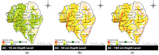
Figure 2.
Spatial distribution of attenuation capacity (AC) in Namyangju at (a) 10 cm, (b) 50 cm, and (c) 100 cm.
Note that the AC maps show distinct patterns through the depth. In general, the topsoil showed higher AC than the one from the subsoils. In addition, ACs near water bodies were relatively low due to the uneven distribution of constituting parameters; OM and TP tend to have lower ratings near water bodies, while SD is higher. As both OM and TP have the highest weight in AC estimation, the lower value of these parameters results in a lower AC. In addition to that, SD has a negative effect on AC, and thus, a higher rating in SD will further decrease the resulting AC (Figure S3).
3.3. SD and AC Variation under Transient Conditions
As aforementioned, SD is a parameter that is constantly changing, which might also affect the overall AC in Namyangju. These changes can be assessed by comparing the SD and AC between time snaps, e.g., 1997 vs. 2022, January vs. June, etc. This kind of comparison is able to present the difference between time snaps, yet it is unable to incorporate the changes happening in between the time snaps and thus might yield a less accurate trend happening over time. By incorporating EHSA into the vulnerability analysis, such problems can be addressed. The end result of applying EHSA is that the overall relative trend of SD and AC in both space and time is obtained. Instead of comparing between time snaps (e.g., 1997 vs. 2022), EHSA considers the whole time period (e.g., 1997–2022) and reports back the trend happening over the time period.
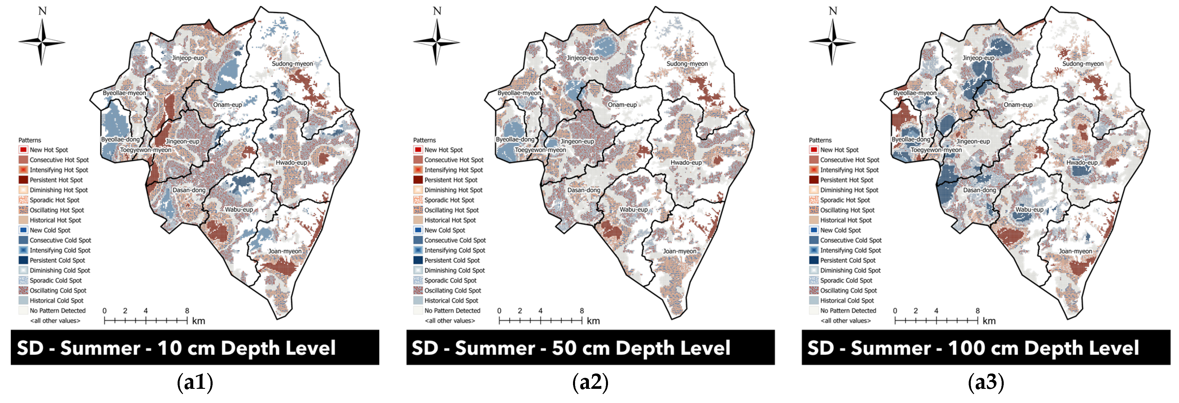
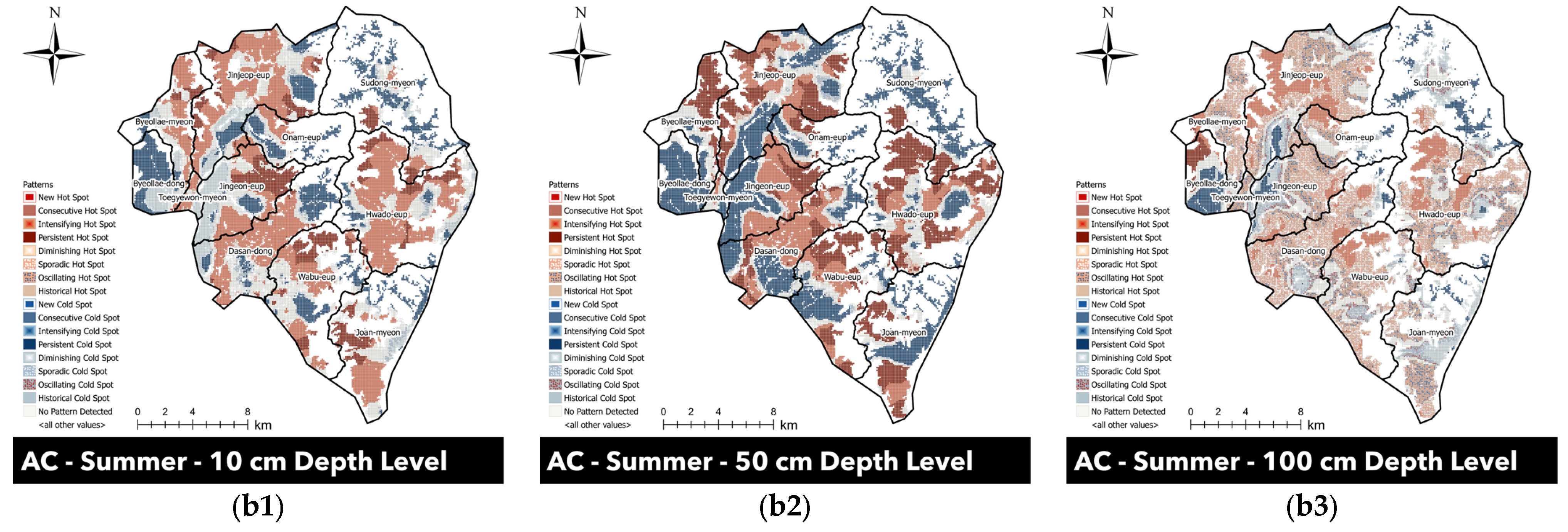
The EHSA results of both SD and AC at 10 cm, 50 cm, and 100 cm are presented in Figure 3. A visual comparison between images in Figure 3 shows that at a depth of 100 cm, there seems to be a larger number of areas corresponding to persistent SD trends, especially for the cold spots. Contrary to the depth of 100 cm, the 50 cm depth has the least persistent SD trends. At both 10 cm and 50 cm, the pattern of SD is dominated by oscillating trends. However, EHSA results for AC show a more prominent persistent trend at 50 cm, while the 100 cm depth is dominated by oscillating and sporadic trends. Cold spots also seem to consistently show up near water bodies (southern part of Jinjeop-eup, eastern part of Toegyewon-myeon, and western part of Jingeon-eup), the western part of Namyangju (Byeollae-dong), and Sudong-myeon. Table 3 provides data on the percent area of each trend pattern at each depth for both SD and AC (based on Figure 3). Around 16% correspond to both persistent cold and hot spots at a 100 cm depth, while only ±10% and ±3% correspond to the persistent trends at the 10 and 50 cm depths, respectively. This result agrees with the general knowledge that water content is less transient at a deeper level. It is also shown that around 63% of the area at 10 cm and 62% of the area at 50 cm show transient oscillating and sporadic trends compared to only ±50% at 100 cm. However, it has to be highlighted that fewer areas with transient trends and a domination of persistent trends should be expected at a deeper level. The domination of resulting transient patterns most probably corresponds to the varying soil porosity along the depth.
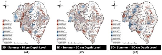

Figure 3.
Emerging hot spot analysis results for summer (a1–a3) saturation degree (SD) and (b1–b3) attenuation capacity (AC) in Namyangju at (a1,b1) 10 cm, (a2,b2) 50 cm, and (a3,b3) 100 cm.
Table 3.
Area (%) of emerging hot spot (HS) and cold spot (CS) trends of saturation degree and attenuation capacity in summer at each depth.
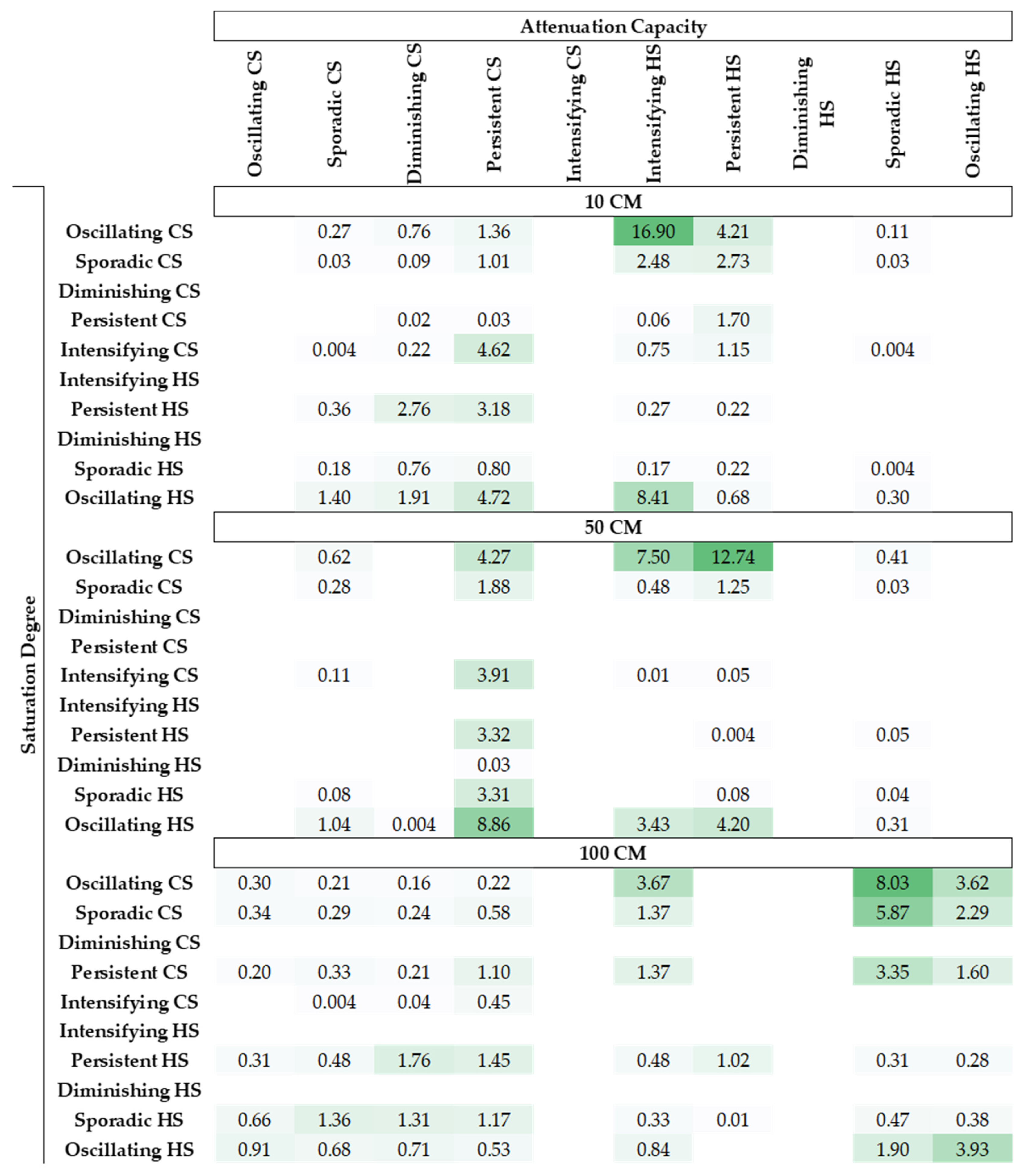
Furthermore, we can investigate the effect of temporal changes of SD on AC in the summer season by comparing the overlapping areas of the same trend between SD and AC (Figure 3). The expected ideal relationship between SD and AC is a negative one, where the cold spot area in SD will return to a hot spot area in AC. Based on the overlapping area presented in Figure 4, only around 6%, 3%, and 13% of the areas return the ideal opposite relationship between SD and AC at depth of 10, 50, and 100 cm, respectively.
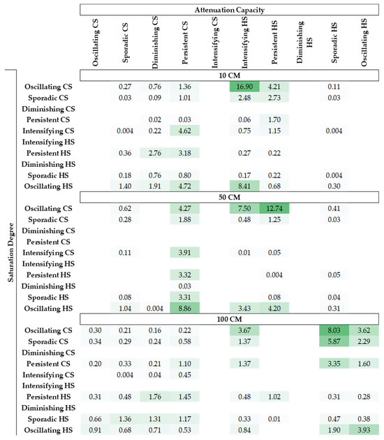
Figure 4.
Overlapping area (%) of spatiotemporal hot spot (HS) and cold spot (CS) patterns of saturation degree and attenuation capacity in summer. The color scheme represents the percentage of the area from smallest (white) to largest (dark green).
The ideal relationship here is when a persistent cold spot in SD returns as a persistent hot spot in AC or an intensifying hot spot in SD returns as an intensifying cold spot in AC, and so forth for the other trends. Despite that, the generally negative correlation between SD and AC still pertains to the overall cold spot and hot spot groups with 46%, 39%, and 42% area (at 10, 50, and 100 cm respectively), showing an overall trend where cold spot SD comes back as hot spot AC and vice versa. In addition, it is also shown that there is about 17% of the area at each depth level that denies the relationship between SD and AC. Although further investigation of the underlying reason for such trends is out of the scope of this study, it is most likely due to the other five governing factors in AC quantification overpowering the effect of SD in the final results.
In general, by incorporating both water flow simulation and EHSA, more insight into vadose zone vulnerability dynamics can be observed. If only a static or single value of SD is used as an input in the attenuation capacity of the vadose zone against diesel, a spatial distribution of areas with a relatively higher or lower AC might give some information and insight into where contamination mitigation and treatment strategies or stricter policies regarding diesel might be needed. Adding EHSA to such vulnerability studies provides an extra urgency factor, which helps in prioritizing areas with notable diminishing hot spots and/or intensifying cold spot trends, as both indicate a worsening vulnerability (to diesel) status over the period of study. EHSA will also help in determining which areas are improving (noted by an intensifying hot spot and diminishing cold spot), which areas require monitoring over time due to a persistent cold spot trend, and which areas are relatively more resilient to diesel contamination (persistent hot spot).
4. Conclusions
This study applied an empirical model describing soil AC against diesel within a GIS environment. Six governing parameters, notably SOM, TP, D30, Cu, n, and SD, were used to determine the spatial distribution of AC in Namyangju. Since SD is highly sensitive to meteorological and climatological changes, the temporal changes (and trends) of both SD and the resulting AC could be captured by incorporating EHSA into the designated time frame (1997–2022). For this purpose, infiltration simulation using Phydrus was performed to obtain simulated historical soil water content subsequently used in SD and AC estimations over time. By applying EHSA, the trends of SD and AC over space and time could be effectively identified. Areas with intensifying cold spots and diminishing hot spots that correspond to the decreasing AC might need stricter policies regarding diesel contamination prevention and mitigation strategies (e.g., areas near water bodies). On the other hand, areas with intensifying hot spots and diminishing cold spots that correspond to the increasing AC might not need a policy that is as strict. The overlapping analysis between SD and AC revealed that the inherent negative correlation between SD and AC still pertains to the overall cold spot and hot spot groups with a small exception (ca. 17%) in which the SD and AC are proportional to each other, presumably due to the uneven distribution of the other five governing factors. Another limitation in this study is the difficulty of model calibration due to the fact that the AC is not directly measurable from the field. Due to this limitation, we focused more on proposing the conceptual framework in a way that incorporates EHSA in vulnerability studies to statistically analyze the vulnerability trend in space and time simultaneously and continuously.
Supplementary Materials
The following supporting information can be downloaded at: https://www.mdpi.com/article/10.3390/hydrology11020019/s1, Figure S1: Daily precipitation (mm) record in Namyangju from 1997–2022; Figure S2: 46 soil series in the studied area; Figure S3: Rated static parameter spatial distribution maps (a) OM, (b) TP, (c) D30, (d) Cu, (e) n in Namyangju at (1) 10 cm, (2) 50 cm, (3) 100 cm; Figure S4: left) Sampling point (red dot), right) Sampling process; Figure S5. The sampling point (red dot) shown in the AC map and the corresponding AC value generated from public data; Table S1: Minimum and maximum values for parameters and the attenuation capacity before normalization; Table S2: Parameter rating, weight, and AC of field sample; Text S1.
Author Contributions
The authors made fairly equal contributions to this manuscript. L.S. and J.C. conceived and conceptualized the study. L.S. and K.-J.L. collected and processed the data. L.S. and J.C. drafted the manuscript. J.C. provided supervision. S.J.K. contributed to methodology. H.Y.J. provided resources. S.H.K. and S.L. made revisions and improvements to the draft. All authors have read and agreed to the published version of the manuscript.
Funding
This work was supported by the Korea Environment Industry & Technology Institute (KEITI) through the Subsurface Environment Management (SEM) Project (2018002440006 and 2021002470004), which is funded by the Korea Ministry of Environment (MOE). The authors also acknowledge support from the Future Research Program (2E33081) and K-Lab (Geo-SMaRT; 2E33084), which are funded by the Korea Institute of Science and Technology (KIST).
Data Availability Statement
The soil physicochemical data analyzed in this article are available on the Korea Rural Development Association (RDA) official website: http://soil.rda.go.kr/ (accessed on 9 June 2022). The meteorological data are available on the Korea Meteorological Administration (KMA) official website: https://data.kma.go.kr/ (accessed on 9 February 2023). The rest of the data presented in this study are available on request from the corresponding author.
Conflicts of Interest
The authors declare no conflicts of interest.
References
- An, S.; Kim, K.; Woo, H.; Yun, S.T.; Chung, J.; Lee, S. Coupled Effect of Porous Network and Water Content on the Natural Attenuation of Diesel in Unsaturated Soils. Chemosphere 2022, 302, 134804. [Google Scholar] [CrossRef]
- Bento, F.M.; Camargo, F.A.O.; Okeke, B.C.; Frankenberger, W.T. Comparative Bioremediation of Soils Contaminated with Diesel Oil by Natural Attenuation, Biostimulation and Bioaugmentation. Bioresour. Technol. 2005, 96, 1049–1055. [Google Scholar] [CrossRef]
- Regadío, M.; Ruiz, A.I.; Rodríguez-Rastrero, M.; Cuevas, J. Containment and Attenuating Layers: An Affordable Strategy That Preserves Soil and Water from Landfill Pollution. Waste Manag. 2015, 46, 408–419. [Google Scholar] [CrossRef]
- Šimůnek, J.; Šejna, M.A.; Saito, H.; Sakai, M.; Van Genuchten, M.T. The HYDRUS-1D Software Package for Simulating the Movement of Water, Heat, and Multiple Solutes in Variably Saturated Media; Version 4.17; Department of Environmental Sciences, University of California Riverside: Riverside, CA, USA.
- Aller, L.; Bennett, T.; Lehr, J.H.; Petty, R.J.; Hackett, G. DRASTIC: A Standardized Method for Evaluating Ground Water Pollution Potential Using Hydrogeologic Settings; U.S. Environmental Protection Agency: Washington, DC, USA, 1987; p. 455.
- Busico, G.; Alessandrino, L.; Mastrocicco, M. Denitrification in Intrinsic and Specific Groundwater Vulnerability Assessment: A Review. Appl. Sci. 2021, 11, 657. [Google Scholar] [CrossRef]
- Douglas, S.H.; Dixon, B.; Griffin, D. Assessing the Abilities of Intrinsic and Specific Vulnerability Models to Indicate Groundwater Vulnerability to Groups of Similar Pesticides: A Comparative Study. Phys. Geogr. 2018, 39, 487–505. [Google Scholar] [CrossRef]
- Andersen, L.J.; Gosk, E. Applicability of Vulnerability Maps. Environ. Geol. Water Sci. 1989, 13, 39–43. [Google Scholar] [CrossRef]
- Woo, H.; An, S.; Kim, K.; Park, S.; Oh, S.; Kim, S.H.; Chung, J.; Lee, S. A New Evaluation Model for Natural Attenuation Capacity of Vadose Zone against Petroleum Contaminants. J. Soil Groundw. Environ. 2022, 27, 92–98. [Google Scholar] [CrossRef]
- Chai, R.; Mao, J.; Chen, H.; Wang, Y.; Shi, X.; Jin, M.; Zhao, T.; Hoffman, F.M.; Ricciuto, D.M.; Wullschleger, S.D. Human-Caused Long-Term Changes in Global Aridity. npj Clim. Atmos. Sci. 2021, 4, 65. [Google Scholar] [CrossRef]
- Lu, J.; Carbone, G.J.; Grego, J.M. Uncertainty and Hotspots in 21st Century Projections of Agricultural Drought from CMIP5 Models. Sci. Rep. 2019, 9, 4922. [Google Scholar] [CrossRef] [PubMed]
- Wang, Y.; Mao, J.; Hoffman, F.M.; Bonfils, C.J.W.; Douville, H.; Jin, M.; Thornton, P.E.; Ricciuto, D.M.; Shi, X.; Chen, H.; et al. Quantification of Human Contribution to Soil Moisture-Based Terrestrial Aridity. Nat. Commun. 2022, 13, 6848. [Google Scholar] [CrossRef]
- Lian, X.; Piao, S.; Chen, A.; Huntingford, C.; Fu, B.; Li, L.Z.X.; Huang, J.; Sheffield, J.; Berg, A.M.; Keenan, T.F.; et al. Multifaceted Characteristics of Dryland Aridity Changes in a Warming World. Nat. Rev. Earth Environ. 2021, 2, 232–250. [Google Scholar] [CrossRef]
- Margono, B.A.; Potapov, P.V.; Turubanova, S.; Stolle, F.; Hansen, M.C. Primary Forest Cover Loss in Indonesia over 2000–2012. Nat. Clim. Change 2014, 4, 730–735. [Google Scholar] [CrossRef]
- ESRI. How Emerging Hot Spot Analysis Works; Environmental Systems Research Institute: Redlands, CA, USA, 2023; Available online: https://pro.arcgis.com/en/pro-app/latest/tool-reference/space-time-pattern-mining/learnmoreemerging.htm (accessed on 14 November 2022).
- Naqvi, S.A.A.; Sajjad, M.; Waseem, L.A.; Khalid, S.; Shaikh, S.; Kazmi, S.J.H. Integrating Spatial Modelling and Space–Time Pattern Mining Analytics for Vector Disease-Related Health Perspectives: A Case of Dengue Fever in Pakistan. Int. J. Environ. Res. Public Health 2021, 18, 12018. [Google Scholar] [CrossRef] [PubMed]
- Purwanto, P.; Utaya, S.; Handoyo, B.; Bachri, S.; Astuti, I.S.; Sastro, K.; Utomo, B.; Aldianto, Y.E. Spatiotemporal Analysis of COVID-19 Spread with Emerging Hotspot Analysis and Space-Time Cube Models in East Java, Indonesia. ISPRS Int. J. Geo Inf. 2021, 10, 133. [Google Scholar] [CrossRef]
- Kang, Y.; Cho, N.; Son, S. Spatiotemporal Characteristics of Elderly Population’s Traffic Accidents in Seoul Using Space-Time Cube and Space-Time Kernel Density Estimation. PLoS ONE 2018, 13, e0196845. [Google Scholar] [CrossRef] [PubMed]
- Xu, D.; Zhang, Q.; Ding, Y.; DE ZHANG, A. Spatiotemporal Pattern Mining of Drought in the Last 40 Years in China Based on the Spei and Space–Time Cube. J. Appl. Meteorol. Climatol. 2021, 60, 1219–1230. [Google Scholar] [CrossRef]
- Lal, P.; Shekhar, A.; Gharun, M.; Das, N.N. Spatiotemporal Evolution of Global Long-Term Patterns of Soil Moisture. Sci. Total Environ. 2023, 867, 161470. [Google Scholar] [CrossRef] [PubMed]
- Ahmadi, H.; Argany, M.; Ghanbari, A.; Ahmadi, M. Visualized Spatiotemporal Data Mining in Investigation of Urmia Lake Drought Effects on Increasing of PM10 in Tabriz Using Space-Time Cube (2004–2019). Sustain. Cities Soc. 2022, 76, 103399. [Google Scholar] [CrossRef]
- Harris, N.L.; Goldman, E.; Gabris, C.; Nordling, J.; Minnemeyer, S.; Ansari, S.; Lippmann, M.; Bennett, L.; Raad, M.; Hansen, M.; et al. Using Spatial Statistics to Identify Emerging Hot Spots of Forest Loss. Environ. Res. Lett. 2017, 12, 024012. [Google Scholar] [CrossRef]
- Betty, E.L.; Bollard, B.; Murphy, S.; Ogle, M.; Hendriks, H.; Orams, M.B.; Stockin, K.A. Using Emerging Hot Spot Analysis of Stranding Records to Inform Conservation Management of a Data-Poor Cetacean Species. Biodivers. Conserv. 2020, 29, 643–665. [Google Scholar] [CrossRef]
- Cuba, N.; Sauls, L.A.; Bebbington, A.J.; Bebbington, D.H.; Chicchon, A.; Marimón, P.D.; Diaz, O.; Hecht, S.; Kandel, S.; Osborne, T.; et al. Emerging Hot Spot Analysis to Indicate Forest Conservation Priorities and Efficacy on Regional to Continental Scales: A Study of Forest Change in Selva Maya 2000–2020. Environ. Res. Commun. 2022, 4, 071004. [Google Scholar] [CrossRef]
- Yang, M.; Yang, Y.S.; Du, X.; Cao, Y.; Lei, Y. Fate and Transport of Petroleum Hydrocarbons in Vadose Zone: Compound-Specific Natural Attenuation. Water Air Soil Pollut. 2013, 224, 1439. [Google Scholar] [CrossRef]
- Mills, S.A.; Frankenberger, W.T. Evaluation of Phosphorus Sources Promoting Bioremediation of Diesel Fuel in Soil. Bull. Environ. Contam. Toxicol. 1994, 53, 280–284. [Google Scholar] [CrossRef] [PubMed]
- R Core Team. R: A Language and Environment for Statistical Computing; R Foundation for Statistical Computing: Vienna, Austria, 2022. [Google Scholar]
- Van Bemmelen, J. Über die Bestimmung des Wassers, des Humus, des Schwefels, der in den Colloïdalen Silikaten Gebundenen Kieselsäure, des Mangans usw im Ackerboden. Landwirthschaftlichen Vers. Station. 1890, 37, 279–290. [Google Scholar]
- Pribyl, D.W. A Critical Review of the Conventional SOC to SOM Conversion Factor. Geoderma 2010, 156, 75–83. [Google Scholar] [CrossRef]
- Hou, E.; Chen, C.; Luo, Y.; Zhou, G.; Kuang, Y.; Zhang, Y.; Heenan, M.; Lu, X.; Wen, D. Effects of Climate on Soil Phosphorus Cycle and Availability in Natural Terrestrial Ecosystems. Glob. Change Biol. 2018, 24, 3344–3356. [Google Scholar] [CrossRef]
- Van Genuchten, M.T.; Schaap, M.G.; Leij, F.J. Rosetta: A Computer Program for Estimating Soil Hydraulic Parameters with Hierarchical Pedotransfer Functions. J. Hydrol. 2001, 251, 164–176. [Google Scholar]
- Vereecken, H.; Weynants, M.; Javaux, M.; Pachepsky, Y.; Schaap, M.G.; van Genuchten, M.T. Using Pedotransfer Functions to Estimate the van Genuchten-Mualem Soil Hydraulic Properties: A Review. Vadose Zone J. 2010, 9, 795–820. [Google Scholar] [CrossRef]
- Robinson, D.A.; Nemes, A.; Reinsch, S.; Radbourne, A.; Bentley, L.; Keith, A.M. Global Meta-Analysis of Soil Hydraulic Properties on the Same Soils with Differing Land Use. Sci. Total Environ. 2022, 852, 158506. [Google Scholar] [CrossRef] [PubMed]
- Šimůnek, J.; van Genuchten, M.T.; Šejna, M. Development and Applications of the HYDRUS and STANMOD Software Packages and Related Codes. Vadose Zone J. 2008, 7, 587–600. [Google Scholar] [CrossRef]
- Collenteur, R.; Vremec, M.; Brunetti, G. Interfacing FORTAN Code with Python: An Example for the Hydrus-1D Model. In Proceedings of the EGU General Assembly, Online, 3–8 May 2020. [Google Scholar]
- Chen, Y.; Guan, Y.; Shao, G.; Zhang, D. Investigating Trends in Streamflow and Precipitation in Huangfuchuan Basin with Wavelet Analysis and the Mann-Kendall Test. Water 2016, 8, 77. [Google Scholar] [CrossRef]
- Ali, R.; Kuriqi, A.; Abubaker, S.; Kisi, O. Long-Term Trends and Seasonality Detection of the Observed Flow in Yangtze River Using Mann-Kendall and Sen’s Innovative Trend Method. Water 2019, 11, 1855. [Google Scholar] [CrossRef]
- Baig, M.R.I.; Shahfahad; Naikoo, M.W.; Ansari, A.H.; Ahmad, S.; Rahman, A. Spatio-Temporal Analysis of Precipitation Pattern and Trend Using Standardized Precipitation Index and Mann–Kendall Test in Coastal Andhra Pradesh. Model. Earth Syst. Environ. 2022, 8, 2733–2752. [Google Scholar] [CrossRef]
- Noori, R.; Woolway, R.I.; Saari, M.; Pulkkanen, M.; Kløve, B. Six Decades of Thermal Change in a Pristine Lake Situated North of the Arctic Circle. Water Resour. Res. 2022, 58, e2021WR031543. [Google Scholar] [CrossRef]
- Noori, R.; Maghrebi, M.; Jessen, S.; Bateni, S.M.; Heggy, E.; Javadi, S.; Noury, M.; Pistre, S.; Abolfathi, S.; AghaKouchak, A. Decline in Iran’s Groundwater Recharge. Nat. Commun. 2023, 14, 6674. [Google Scholar] [CrossRef]

Disclaimer/Publisher’s Note: The statements, opinions and data contained in all publications are solely those of the individual author(s) and contributor(s) and not of MDPI and/or the editor(s). MDPI and/or the editor(s) disclaim responsibility for any injury to people or property resulting from any ideas, methods, instructions or products referred to in the content. |
© 2024 by the authors. Licensee MDPI, Basel, Switzerland. This article is an open access article distributed under the terms and conditions of the Creative Commons Attribution (CC BY) license (https://creativecommons.org/licenses/by/4.0/).