Article

An Integrated Framework to Assess the Environmental and Economic Impact of Fertilizer Restrictions in a Nitrate-Contaminated Aquifer

School of Civil Engineering, Aristotle University of Thessaloniki, GR54124 Thessaloniki, Greece
*
Author to whom correspondence should be addressed.
Hydrology 2024, 11(1), 8; https://doi.org/10.3390/hydrology11010008
Submission received: 5 December 2023 / Revised: 30 December 2023 / Accepted: 2 January 2024 / Published: 4 January 2024
(This article belongs to the Special Issue Groundwater Pollution: Sources, Mechanisms, and Prevention)

Abstract

:
Groundwater nitrate contamination caused by the excessive use of nitrogen-based fertilizers has been widely recognized as an issue of significant concern in numerous rural areas worldwide. To mitigate nitrate contamination, corrective management practices, such as regulations on fertilizer usage, should be implemented. However, these measures often entail economic consequences that impact farmers’ income, and thus should be properly assessed. Within this context, an integrated framework combining the environmental and economic assessment of fertilization restrictions through multi-criteria decision analysis is presented in an effort to efficiently manage groundwater nitrate contamination in rural areas. For this task, various scenarios involving reductions (10%, 20%, 30%, 40% and 50%) in fertilizer application were investigated, evaluated and ranked in order to determine the most suitable option. The environmental assessment considered occurrences of nitrates in groundwater, with a specific emphasis on nitrate concentrations in water-supply wells, as obtained by a nitrate fate and transport model, while the economic analysis focused on the losses experienced by farmers due to the reduced fertilizer usage. Our case-study implementation showed that a 30% reduction in fertilization is the most appropriate option for the area being studied, highlighting the importance of adopting such an approach when confronted with conflicting outcomes among alternatives.

1. Introduction

Nitrate is generally considered one of the most widespread and persistent pollutants found in groundwater, originating from multiple nitrogen sources, primarily related to human activities, and to a lesser extent, to natural processes [1,2,3,4,5]. Anthropogenic sources mainly include agricultural activities such as fertilizer and manure applications and animal feedlot operations, as well as industrial and sewage discharges. Natural sources like decomposing organic matter or atmospheric nitrogen deposition also contribute to nitrate occurrence in groundwater, but anthropogenic sources tend to have a more pronounced impact due to their scale and intensity [1,6,7,8,9,10]. Among various human nitrate sources, agricultural activities, and especially the use of nitrogen-rich fertilizers for enhancing crop productivity, have been recognized as the main cause of groundwater nitrate contamination worldwide, posing a serious threat to rural areas [8,11,12,13,14].
Concerns over nitrate contamination further increase in regions where groundwater is used for human consumption [4,15,16], since elevated nitrate levels in drinking water have been linked to adverse health issues, such as methemoglobinemia in infants and stomach cancer in adults [8,17,18,19,20], although this connection remains a topic of controversy [21,22]. As a result, the Drinking Water Directive (98/83/EC) and the World Health Organization (WHO) set a maximum allowable nitrate concentration limit of 50 mg/L, along with an indicative threshold of 25 mg/L, defined as the “guidance value”, in order to prevent potential health consequences resulting from the prolonged consumption of nitrate-contaminated water [19,23]. Beyond concerns for public health, excessive nitrate concentrations can also induce serious environmental harm particularly within natural ecosystems by leading to the eutrophication of interconnected surface water bodies [3,5,24,25].
In this context, it is notably important to adopt and implement corrective management practices aimed at preventing nitrate contamination caused by the excessive usage of agricultural fertilizers, which also aligns with all relevant European legislation, such as the Nitrates Directive (91/676/EEC), the Water Framework Directive (2000/60/EC), and the Groundwater Directive (2006/118/EC), as well as with the objectives outlined in the UN Sustainable Development Goals (SDGs), and especially those of SDG 6. According to SDG 6, access to safe and affordable drinking water for everyone by 2030 has to be ensured by reducing water pollution, which involves, among other things, the mitigation of groundwater nitrate contamination [26,27,28]. In general, imposing restrictions on the usage of nitrogen-based fertilizers—which is actually translated to reducing fertilizer application rate and thus limiting nitrogen input into the soil and nitrate leaching into groundwater—is a common and effective practice applied in the effort of controlling nitrate contamination in rural areas [8,29,30,31,32]; apparently, the higher the reduction in the rate of fertilizer application is, the greater the decrease in nitrate contamination levels might be, thus increasing the likelihood of reaching or maintaining compliance with established groundwater quality standards.
However, implementing effective management alternatives requires a comprehensive consideration of the groundwater system, along with a proper assessment of their efficiency in achieving the desired goals [32,33,34]. In this context, numerical modelling is usually implemented to investigate and evaluate the effectiveness of management practices on nitrate occurrences in groundwater. Numerical models, by simulating how nitrates move and behave in groundwater over space and time, provide insight into the potential outcomes of protection measures in advance, and they serve as a tool to support science-based policy decisions (i.e., nitrate abatement policies) [25,35,36,37,38]. Several studies have implemented numerical modeling through the development of nitrate fate and transport models to simulate and assess the impact of fertilization regulation practices on nitrate contamination levels (e.g., [14,17,31,32,35,38,39,40]). Other studies (e.g., [25,29,41,42,43]) have expanded their scope beyond the environmental benefits of fertilization regulations by incorporating the potential economic consequences stemming from their implementation into their analysis. Fertilization reduction practices, by having an adverse impact on crop productivity due to decreased yields or hindered crop growth, can result in negative economic ramifications for farmers, noticeably affecting the local economy in rural areas [6,25,35,43]; apparently, the higher the reduction in fertilizer application rate is, the greater the farmers’ economic losses might be.
Based on the preceding analysis, it becomes clear that fertilizer regulations implicitly involve conflicting objectives. These practices actually seek to reduce nitrate concentrations to address environmental concerns, while, at the same time, aiming to minimize the economic losses resulting from their implementation [6,29]. These conflicting objectives can lead to different prioritization schemes when tasked with choosing among various scenarios involving fertilization reduction, i.e., scenarios featuring varying rates of fertilization reduction, since no single scenario, i.e., no certain rate of reduction, can be deemed universally optimal from both environmental and economic perspectives. This complexity necessitates the use of a multi-criteria decision analysis to prioritize the applied fertilization reduction scenarios [2,6]. However, to date, few studies (e.g., [29,43,44]) have undertaken such analysis, generally leading to a lack of decision-support tools for identifying and selecting the most appropriate solutions when designing nitrate abatement policies [23,45].
In this context, the main objective of this work is to develop an integrated decision-support framework aimed at efficiently managing groundwater nitrate contamination caused by fertilizer use in rural areas. More specifically, the framework proposes the most suitable fertilizer regulation policy (i.e., fertilizer reduction scenario) that minimizes the income losses in agriculture resulting from the reduction in nitrogen fertilizer application, while, at the same time, adhering to certain environmental constraints, particularly nitrate contamination levels. The proposed methodology integrates results from a nitrate fate and transport model, and an economic model within a decision analysis framework developed through the Analytic Hierarchy Process (AHP) method, in an effort to establish a connection between fertilization patterns and nitrate concentrations, as well as farmers’ income. This comprehensive analysis can assist policymakers and stakeholders in making informed decisions regarding agricultural practices and regulations, while considering both environmental and economic aspects.

2. Materials and Methods
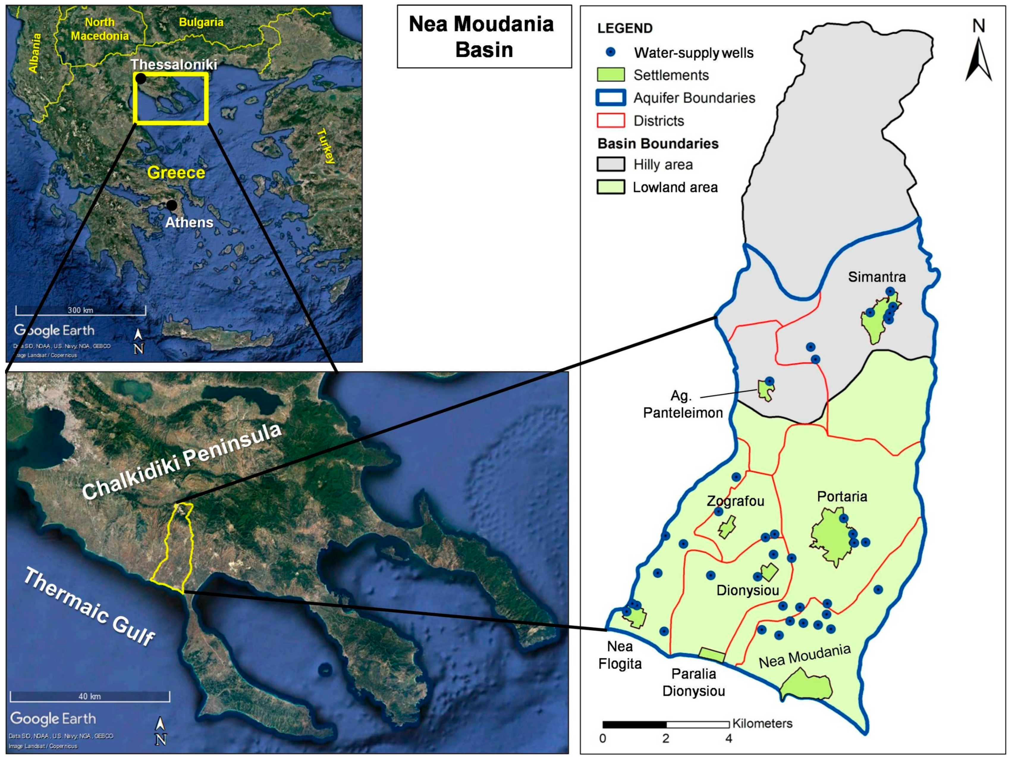
2.1. Study Area

The hydrological basin of Nea Moudania, located in the south-western part of Chalkidiki peninsula, Northern Greece, (south-east of the city of Thessaloniki), was chosen as the study area. It is a coastal basin, directly connected to the sea in the south, where it is surrounded by the Thermaikos Gulf (Figure 1). The basin occupies an area of approximately 127 km2, with a mean topographic elevation of about 176 m above sea level and a mean slope of about 12%. The climate of the study area, which is hydrologically divided into two sub-regions (Figure 1), the lowland area in the south (53.7%) and the hilly area in the north (46.3%), is classified as semi-arid to humid, typically Mediterranean, with an average annual precipitation of 417 mm for the lowland area and 504 mm for the hilly one.
In terms of geology, most of the region belongs to the Peonia geologic zone and, more specifically, to the Moudania geologic formation, which is part of the Neogene deposits detected in western Chalkidiki. In the Moudania formation, which mostly consists of alternated beds of sandstones, sands, silts and red to brick red clays, the main aquifer system of the study area developed (Figure 1) in the form of successive water-bearing layers, separated by lenses of semi-permeable or impermeable materials [46,47]. The Nea Moudania aquifer serves as the primary exploitable aquifer and the sole source of freshwater in the region, used to meet irrigation, domestic and livestock needs.
The study area, as part of the main agricultural area of Chalkidiki (referred to as the “Kalamaria plains”) is a typical rural area, where agriculture holds a dominant role in the local economy. The main crops are wheat, olive and apricot cultivations (about 96% of the total cultivated area), while other crops include barley, vegetables (e.g., tomatoes), pistachios and vineyards. Livestock activities are also present in the region, including cattle, sheep, goat, pig and poultry breeding, but make a relatively small contribution. Regarding the land use allocation, nearly 76% of the Nea Moudania basin is designated as agricultural land, with woodland covering 20% (mostly in the northern part) and the remaining 4% accounting for urban and touristic development. Especially for the latter case, eight settlements are located in the study area, on the basis of which the region is divided into seven administrative districts (two settlements belong to the same district) (Figure 1) [48]. In Table 1, information on the settlements’ total populations (including both permanent and seasonal residents), along with the corresponding number of wells used to provide water to each settlement is contained. Ιn the approach followed in the current study, these wells served as critical receptors for observing nitrate concentrations.
In general, the Nea Moudania aquifer is characterized by severe quantitative degradation, since a substantial decline in groundwater levels is observed as a result of excessive abstraction of groundwater resources, especially for irrigation purposes. In addition, the study area has also experienced groundwater quality deterioration due to seawater intrusion and nitrate contamination, both linked to the intensification of agricultural activities [46,49]. Nitrate contamination has been well-documented in the study area. Latinopoulos (2003) [46], who carried out a groundwater sampling campaign in 34 wells during November 2001, found that, locally, nitrate concentrations have reached values up to 180 mg/L, exceeding the allowable limit of 50 mg/L. The study revealed that higher nitrate values are primarily related to medium-to-low-depth wells (<50 m), and they are mainly detected in the north and central part of the reference area, where intensive agricultural activities and fertilization practices are observed. Siarkos (2015) [48] drew similar conclusions regarding the spatial distribution of nitrate concentrations, attributing higher values to increased agricultural activities taking place in the aforementioned part of the study area. The analysis was based on nitrate concentration measurements in 12 deep wells (>100 m) designated for domestic use between 2011 and 2013. Specifically, it was found that nitrate concentrations in the sampled water-supply wells situated within agricultural areas in the north and central part of the aquifer were close to or exceeded (in one case) the “guidance value” of 25 mg/L, indicating the potential for further increases in concentrations in the coming years. Furthermore, it is worth mentioning that the broader region of the “Kalamaria plains”, part of which is the Nea Moudania basin, has been identified as a “Nitrate Vulnerable Zone (NVZ)”, in line with Nitrates Directive.
Based on the preceding analysis, it can be concluded that nitrate contamination has evolved into a matter of significant concern for the study area, posing a threat not only to the availability of groundwater reserves but also to the local population, thus raising public health issues. In this context, ensuring the protection of groundwater resources’ quality becomes of utmost importance, necessitating the implementation of protective measures, while properly assessing their efficiency. As previously stated, agricultural activities and, more specifically, the application of nitrogen-based fertilizers, have been recognized as the main source of groundwater nitrate contamination in the region, and therefore management practices should target this certain source. However, there are several other potential on-ground nitrogen sources that might contribute to the presence of nitrate in groundwater, including irrigation with nitrogen-contaminated groundwater, leakage from septic systems and wastewater networks (as listed in Table 1 for each settlement), livestock breeding (assumed to be mainly situated within settlements due to the relatively small number of livestock, primarily catering to household needs) and atmospheric deposition. All these sources were considered when calculating the on-ground nitrogen loadings for the nitrate fate and transport model developed in this study.

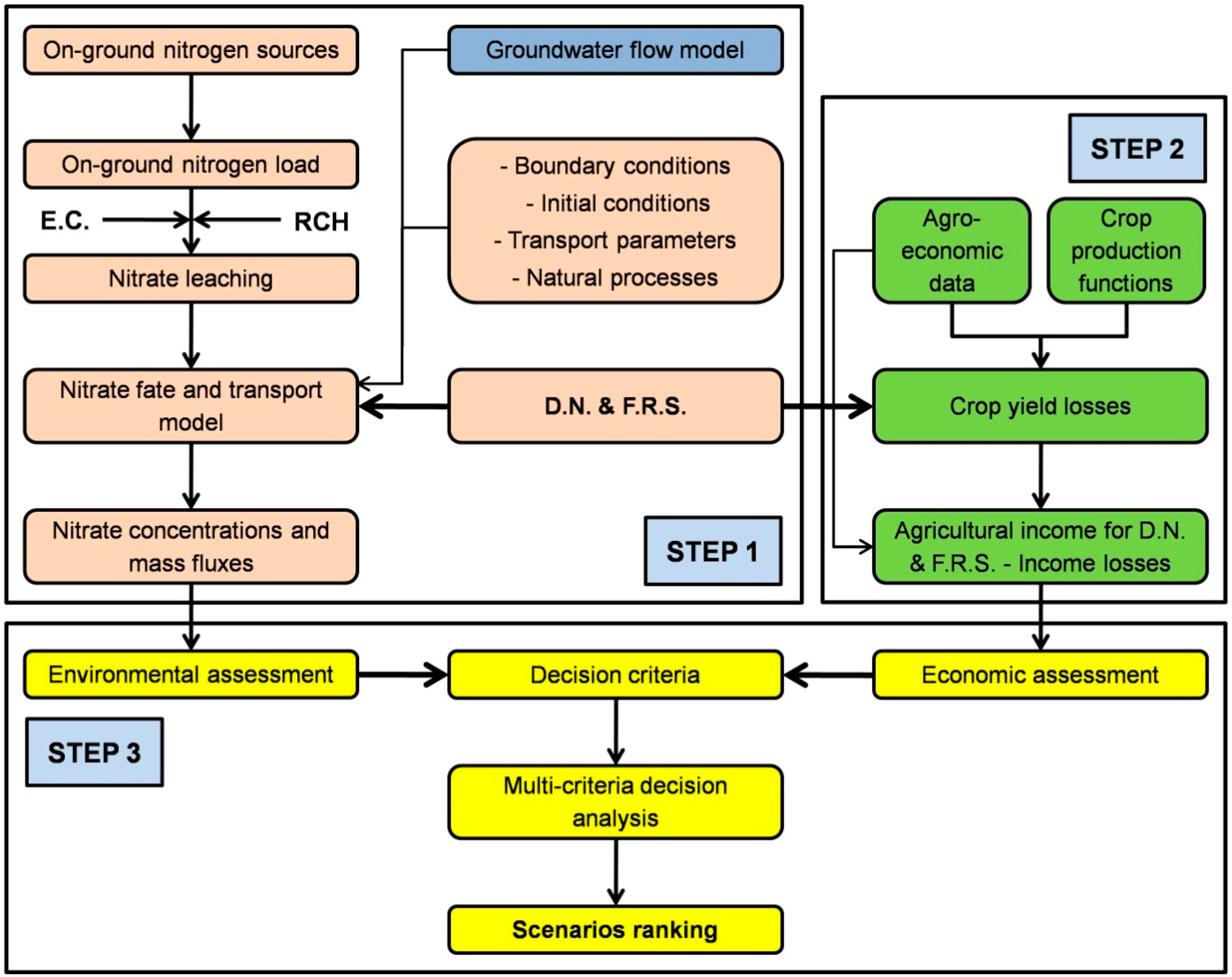
2.2. General Methodological Framework

The methodology followed in the present study is aimed at investigating and evaluating the effect of fertilization reduction as a protective measure against groundwater nitrate contamination with the ultimate goal of providing the best management option, that is the most effective fertilization reduction scenario, taking into account both environmental and economic aspects. More specifically, in terms of the environmental perspective, the study examines the presence of nitrate in local groundwater resources, especially emphasizing nitrate concentrations in water-supply wells, thus accounting for potential risks associated with the consumption of poor-quality water. With respect to the economic point of view, the analysis focuses on estimating the costs of groundwater protection in the agricultural sector, specifically by assessing the productivity losses incurred by farmers as a result of the reduced use of fertilizers. A general view of the proposed methodology is depicted in Figure 2, while its various parts are briefly described in the following:
-
Step 1: Building a nitrate fate and transport model to study the spatial and temporal variations in nitrate concentrations under various scenarios, i.e., do-nothing and fertilization reduction scenarios, as well as to obtain the nitrate values at water-supply wells, for each applied scenario.
-
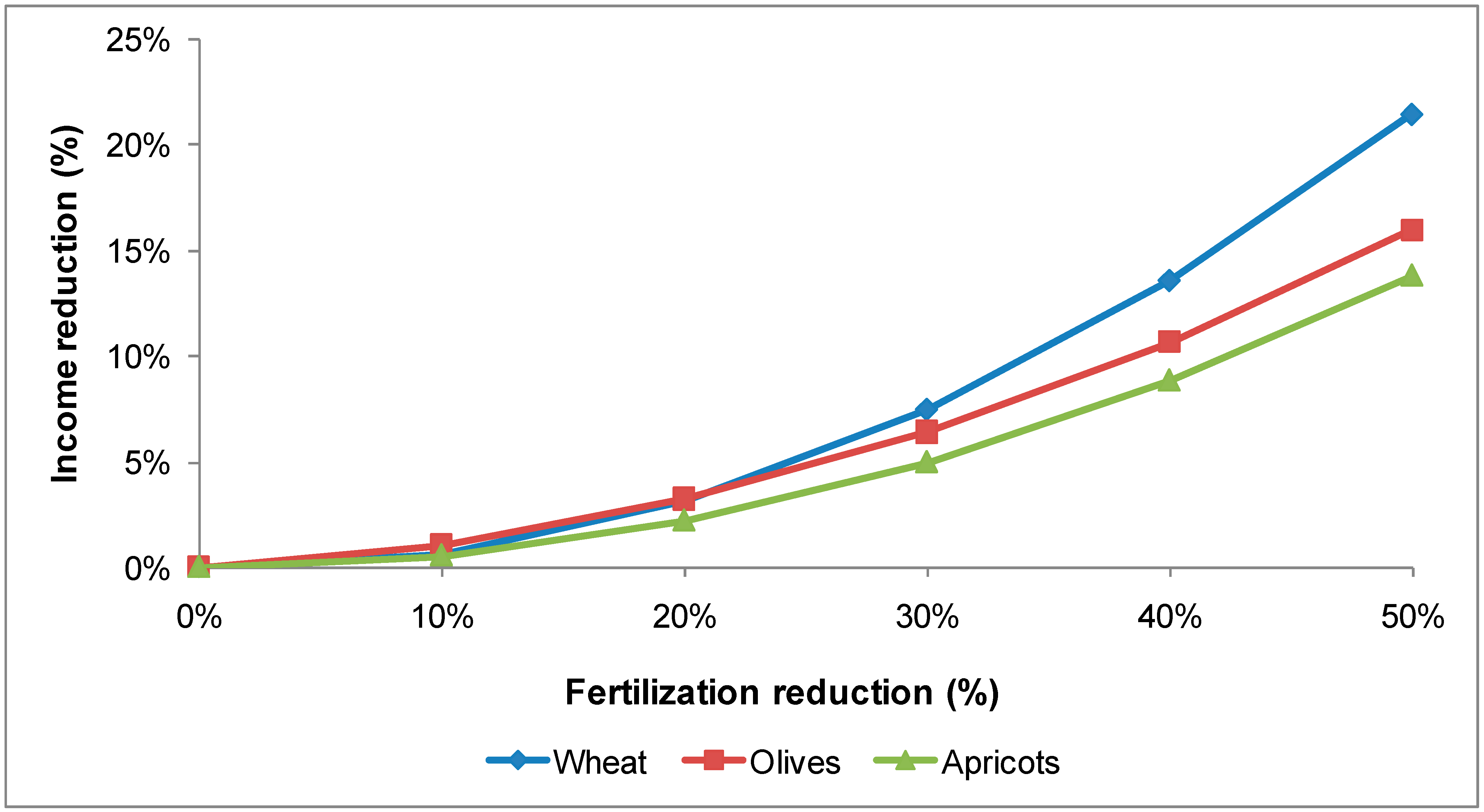
Step 2: Combining crop production functions with agro-economic data to estimate expected crop-yield losses under different fertilization reduction scenarios, while conducting an economic analysis based on cropping patterns and agro-economic data to calculate the agricultural income for both the do-nothing and fertilization reduction scenarios. The difference in agricultural income between the do-nothing scenario and any scenarios involving fertilization restrictions (fertilization reduction scenarios) is considered as the potential income losses associated with the applied scenario.
-
Step 3: Performing a multi-criteria decision analysis subject to a set of criteria derived from both the environmental (from Step 1) and economic (from Step 2) assessment in order to prioritize the proposed fertilization reduction options and eventually select the most suitable that best meets the predefined decision criteria.

2.3. Numerical Modeling

In general, solute mass transport simulation in groundwater requires the simulation of a groundwater flow system as the first step. This is considered essential for determining the hydraulic head distribution and groundwater velocity field throughout the model’s domain, as well as for calculating the fluxes across grid cell interfaces in all directions [19,25,29,50]. In the present study, the development of the nitrate fate and transport model employed to investigate the spatio-temporal variation in nitrate concentrations was based on an existing calibrated/validated transient groundwater flow and transport model [49,51], originally created for simulating seawater intrusion (i.e., chloride transport) in the area of interest. This coupled flow and transport model was built by applying the SEAWAT code [52], thus taking into consideration the effects of density variations on groundwater flow caused by changes in chloride concentrations. The newly formed nitrate fate and transport model was developed by applying the MT3DMS code [53].
Given that the existing model was initially designed to simulate seawater intrusion, several adjustments, primarily associated with solute transport, are required in order to account for the new simulation conditions involving the modeling of nitrate contamination. These modifications are mainly related to the initial and boundary conditions of the transport model, as well as the type of pollution sources and the way the pollutants enter the aquifer. However, certain aquifer parameters linked to solute transport and affecting advection and dispersion of chemical constituents in groundwater, such as effective porosity (ne) and longitudinal and transverse dispersivities (αL, αT), were not subject to modifications due to the prior calibration/validation of the existing model. In the subsequent sections, an overview of the existing groundwater model, mainly focusing on the part related to groundwater flow simulation, is provided, along with a thorough description of the development and calibration of the newly formed nitrate fate and transport model, which is then used to simulate various fertilizer application scenarios.

2.3.1. Overview of the Existing Groundwater Model

Detailed information on the overall modelling procedure, including the construction and calibration/validation of the existing seawater intrusion model, can be found in Siarkos and Latinopoulos (2016) [49] and Siarkos et al. (2017) [51]. However, in the following, an outline of the essential components of the existing groundwater model, especially referring to the aquifer conceptual model and the flow simulation, is provided [49]:
  • The boundaries of the aquifer under study coincide with those of the Nea Moudania basin, with the exception of the northern boundary, which was defined based on an isopiezometric contour map (year 2001) realized by Latinopoulos (2003) [46] by applying the Kriging method (Figure 1);
  • Together, the various successive permeable stratigraphic layers form a single, unified aquifer system with a uniform thickness of 250 m, thus resulting in a vertically integrated two-dimensional areal model comprising one layer in the z-direction;
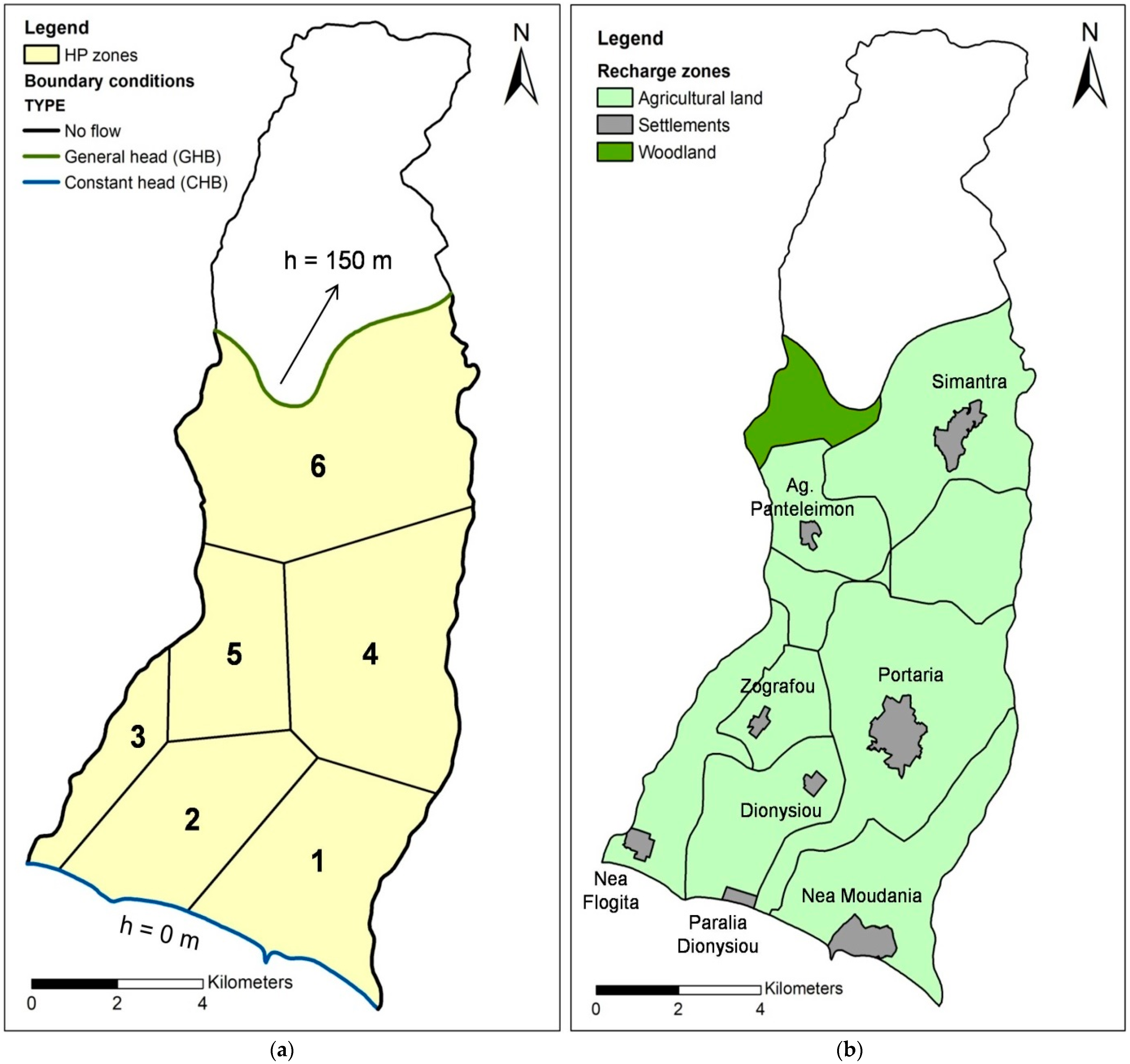
  • The aquifer’s eastern and western boundaries are treated as no-flow boundaries based on the overall arrangement of flow lines on a regional scale [46], whereas the southern and northern boundaries are assigned as constant head boundary (CHB, h = 0 m) and general head boundary (GHB, h = 150 m), respectively (Figure 3a). Regarding the southern boundary, the hydraulic head values remain constant over time, while concerning the northern boundary, the hydraulic head values gradually decrease over time following the overall decline in groundwater levels observed in the region;
  • The study area is divided into six distinct hydro-geological zones (HP zones, Figure 3a) based on a number of pumping tests carried out in individual wells [46]; each of these zones is assigned a different value with regard to various aquifer parameters, such as hydraulic conductivity (K), specific storage (SS), specific yield (Sy) and effective porosity (ne). However, longitudinal and transverse dispersivities (αL, αT) are considered to be constant throughout the region, resulting in the use of a uniform value across the entire model domain. In Table 2, the values of the aforementioned aquifer parameters, as determined through the model calibration/validation procedure, are presented. As already mentioned, especially regarding the transport parameters, i.e., effective porosity and dispersivities, the same values are also used in the case of the nitrate fate and transport model developed in the current study;
  • The aquifer is primarily replenished by rainfall, irrigation return flows and losses from water supply and wastewater networks, with additional recharge taking place at the southern and northern boundaries; particularly concerning the first group of aquifer recharge sources, the study area is divided into several recharge zones (Figure 3b), taking into account factors such as local hydrological conditions, land use types and administrative boundaries within the region;
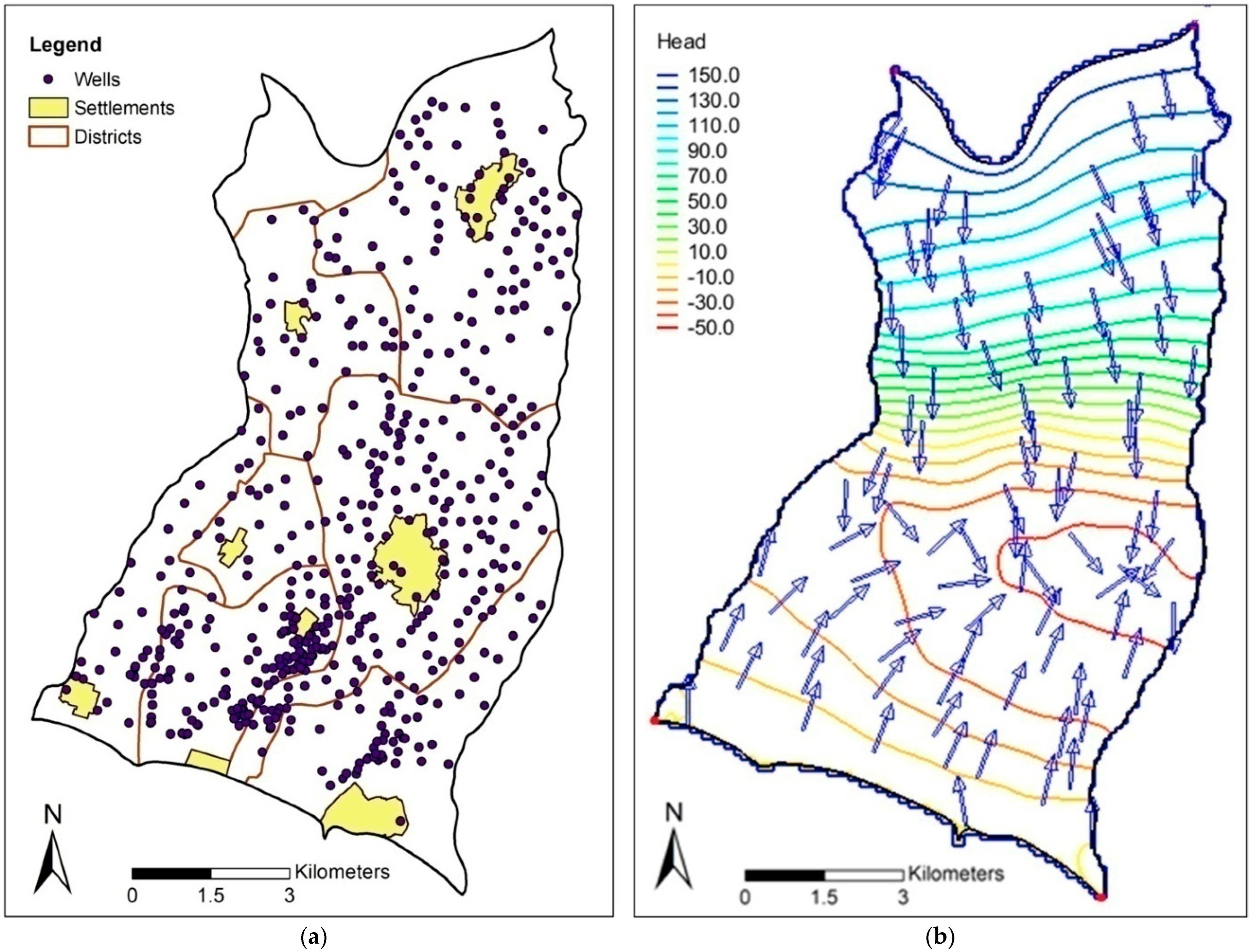
  • The groundwater is abstracted from numerous wells to meet irrigation, domestic and livestock needs (Figure 4a); the pumping rates of the wells vary across municipal districts and specific water uses, under the assumption that each district’s domestic and livestock needs are met by the same wells;
  • The numerical model’s spatial discretization involves the construction of a square grid in the horizontal plane, where cells are uniformly sized (100-m side) across the model domain;
  • The numerical model’s temporal discretization includes: (a) month-long stress periods accounting for the aquifer recharge and withdrawal regimes, (b) a pumping (1 May–30 September, 153 days) and a non-pumping (1 October–30 April, 212 days) period within each year in an effort to incorporate diverse temporal patterns regarding both groundwater abstraction for irrigation and irrigation return flows and (c) a 13-year simulation period (2001–2014) for calibration and validation purposes;
  • The calibration of the flow model was performed using 13 observation wells monitored during November 2002 and 12 observation wells monitored during April 2003 [46] (Mean Error = −0.176 m, Mean Absolute Error = 1.502 m, Root Mean Square Error = 1.735 m and Mean Relative Error = 1.02%), and the validation was performed using 12 observation wells monitored during November 2010 [48] (Mean Error = −0.478 m, Mean Absolute Error = 1.822 m, Root Mean Square Error = 2.059 m and Mean Relative Error = 1.36%). The transport model was calibrated from 2011 to 2014 using chloride concentration measurements from 6 observation wells [48] (Mean Error = −0.10 mg/L, Mean Absolute Error = 6.93 mg/L, Root Mean Square Error = 9.29 mg/L and Mean Relative Error = 3.36%); and,
  • Low hydraulic head values (in relation to the mean sea level) are observed especially in the central part of the Nea Moudania aquifer due to the extensive usage of groundwater within that area (approximately 75% of the total water abstractions originating from this location). As a result, reversal of the natural groundwater flow occurs, leading to the influx of seawater along the coastline (southern boundary) and towards the interior of the aquifer (Figure 4b).

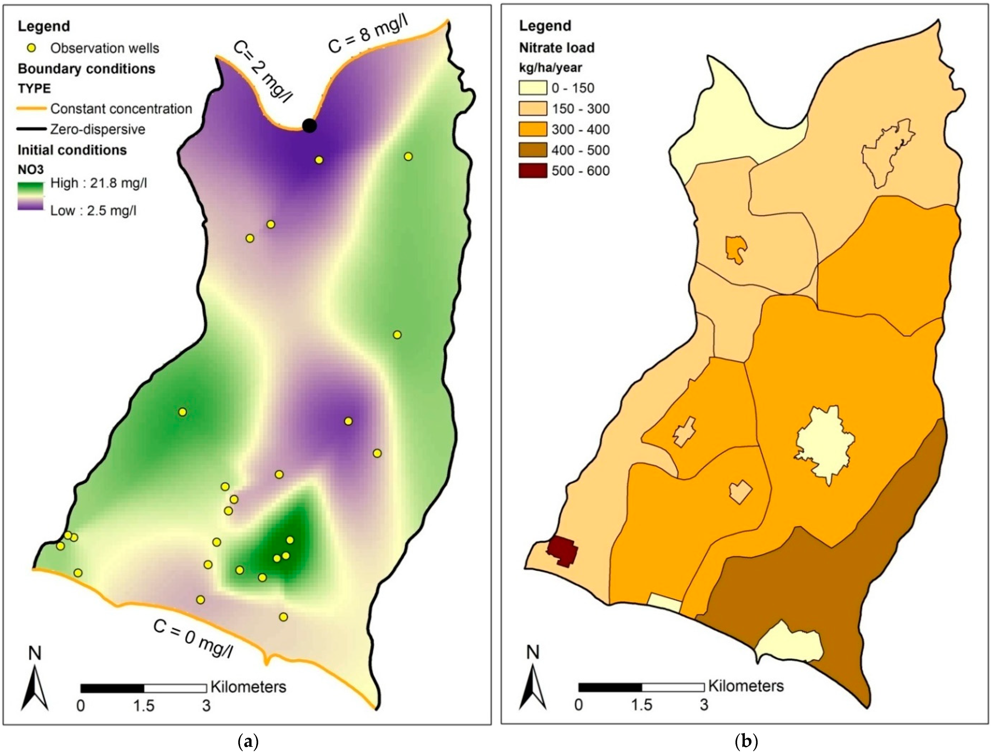
2.3.2. Nitrate Fate and Transport Model Development

In order to build the nitrate fate and transport model, apart from obtaining the velocity field from the groundwater flow model previously presented, the following have to be properly defined (Figure 2, Step 1): (a) the model boundary conditions, that is, specifying the type of boundary conditions for nitrate transport along the aquifer limits, (b) the model initial conditions, that is, determining the spatial distribution of nitrate concentrations at the beginning of the simulation, (c) the amount of nitrate entering the aquifer system, that is, quantifying nitrate leaching from the soil to groundwater, which is directly linked to the on-ground nitrogen loadings deriving from various nitrogen pollution sources, and (d) the physical or chemical processes occurring during the transport of nitrates in groundwater.
At first, the boundary and initial conditions used for the development of the nitrate fate and transport model are illustrated in Figure 5a. Regarding the boundary conditions, the eastern and western boundaries were set as zero-dispersive boundaries, since no flow is observed through these parts of the aquifer (Figure 3a), while the southern and northern boundaries were represented by constant concentration boundaries (CCB). In the case of southern boundary, a zero-nitrate concentration was assigned to it accounting for the inflow of seawater into the aquifer through this boundary. On the other hand, the northern boundary was split into two segments, each designated with a different nitrate concentration (2 mg/L for the left segment and 8 mg/L for the right segment), determined on the basis of the background concentrations observed near the respective segments. In both segments, nitrate concentrations remain constant over time for the entire simulation. With respect to the model initial conditions, i.e., initial nitrate distribution, they were derived by applying the Kriging method to nitrate concentrations measured during November 2001 across 16 monitoring wells [46].
Next, on-ground nitrogen loadings originating from the potential nitrogen sources observed in the study area (see Section 2.1) have to be estimated in order to determine the amount of nitrate leaching entering the groundwater system through infiltration. The calculation of nitrogen loading for each of these sources was performed according to the type of land use it is associated with, while taking into consideration the different municipal districts and settlements within the study area, thus accounting for the spatial distribution of on-ground nitrogen sources and corresponding loadings. Using this approach, also applied to the calculation of groundwater recharge, nitrogen loading was computed at the resolution of individual recharge zone (Figure 3b), thus directly linking the nitrate inputs to the net recharge of each individual zone within the study area [19,36]. Under these conditions, in order to capture, on the one hand, the temporal patterns of groundwater recharge (i.e., monthly time-step) and, on the other hand, the temporal variability in certain nitrogen source applications, e.g., fertilizer application, irrigation, deposition, which generally vary within the year [54], nitrate loading for all nitrogen sources was computed on a monthly basis.
Based on the preceding analysis, nitrogen loading per month at a recharge zone level was determined taking into account the types of nitrogen sources in each zone, in addition to the following information regarding the estimation of the corresponding loading from each source [10,54,55,56]:
-
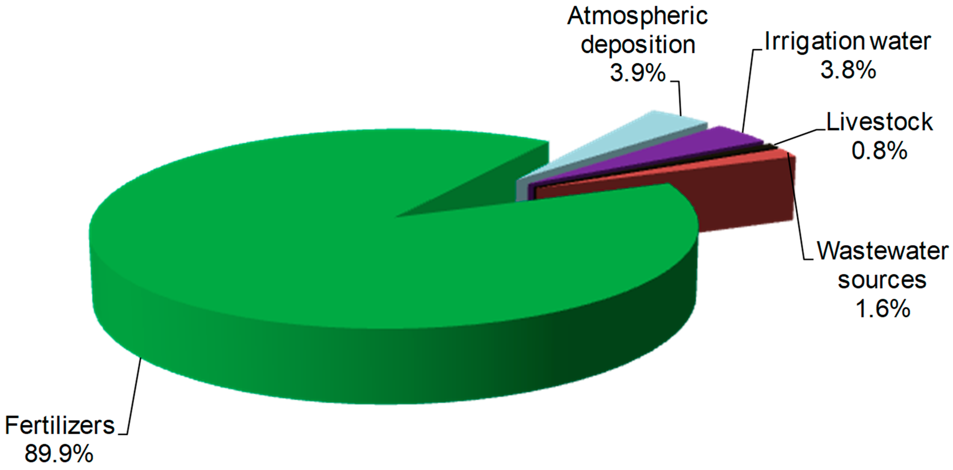
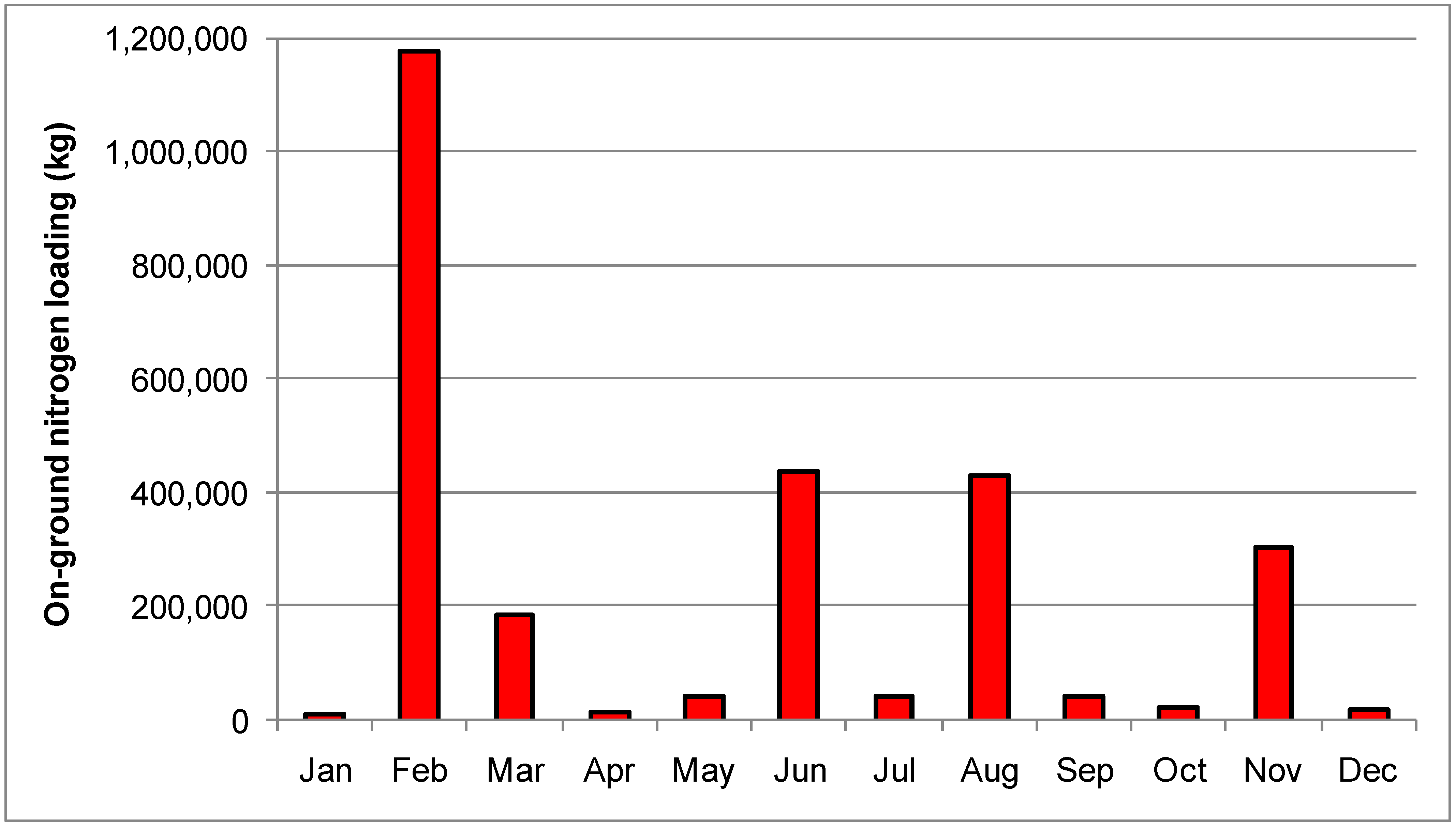
Fertilizers: For the different types of crops spotted in the study area, nitrogen loading from agricultural fertilizers was calculated by multiplying the suggested fertilizer application rate for each crop (kg/ha), as listed in Table 3, with the actual fertilized area, while taking into consideration the fertilizer application timing for each crop, i.e., the specific months in which fertilizers are generally applied.
-
Irrigation water: Nitrogen loading from irrigation water was calculated by multiplying the mean concentration of nitrates (mg/L) in groundwater, as obtained by previous research conducted in the study area [46], with the amount of water used for irrigation, after converting nitrate (NO3) concentrations into nitrate–nitrogen (NO3-N) concentrations.
-
Septic systems: Nitrogen loading from septic systems was calculated by multiplying the corresponding nitrogen production per capita (0.012 kg/d) [54] with the actual population (permanent and seasonal).
-
Wastewater network: Nitrogen loading from wastewater networks was calculated by multiplying the corresponding nitrogen concentration in wastewater (35 mg/L) [58] with the estimated water leakage in the network.
-
Livestock: For the different types of dairy animals detected in the study area, nitrogen loading from livestock was calculated by multiplying the corresponding nitrogen production per head for each animal type (kg/d), as presented in Table 4, with the actual number of animals.
-
Atmospheric deposition (wet): Nitrogen loading from precipitation was calculated by multiplying the mean concentration of nitrogen in precipitation (3.0 mg/L) [60] with the amount of water from precipitation (after subtracting the runoff volumes).
In an effort to provide a comprehensive overview of the spatial and temporal distribution of on-ground nitrogen loading in the region, several key figures based on the aforementioned calculations are provided. More specifically, in Figure 5b and Figure 6, the spatial distribution of annual nitrogen loading at the recharge zone level and the percentage breakdown of nitrogen loadings from the different sources present in the study area are depicted, respectively, while in Figure 7, the monthly variation in nitrogen loading is shown. As is apparent, and in accordance with the findings of previous studies, agricultural fertilizers constitute the predominant nitrogen source in the Nea Moudania aquifer, accounting for approximately 90% of the total nitrogen generated in the area. This clearly suggests that management strategies should be tailored to address this specific source. However, the highest nitrogen loading per hectare (590 kg/ha/year) is observed in an urban area, and more specifically in the settlement of Nea Flogita, due to the presence of septic systems within the settlement (Table 1) and the substantial increase in population during the tourist season. As far as the agricultural areas are concerned, the Nea Moudania district exhibits the highest nitrogen loading per hectare (404 kg/ha/year), primarily due to the notably higher percentage of olive trees (53% of the cultivated land) within the district (nitrogen requirements for olive trees significantly exceed those of other crops, as shown in Table 3). With respect to the temporal variations in nitrogen loading, it is observed that the peak amounts coincide with months mainly dedicated to nitrogen fertilizer application (i.e., February, March, June, August and November). Notably, the highest levels are recorded in February (1.18 × 10⁶ kg), aligning with the primary fertilization period for olive trees.
After calculating nitrogen loading, nitrate loading reaching the groundwater system was determined using the same spatial (per recharge zone) and temporal (per month) resolution. For this task, an export coefficient model was applied, according to which the nitrate loading is calculated as a fraction of the total on-ground nitrogen loading, accounting for the several biochemical transformations of nitrogen occurring in the soil, such as mineralization, immobilization, nitrification, denitrification and plant uptake [17,25,56]. In particular, nitrate loading is calculated by multiplying nitrogen loading with predefined export coefficients depending on the types of nitrogen sources [14,40,54,55,61,62]. The export coefficients adopted in the current study for the different types of nitrogen sources within the area of interest were obtained from relevant literature sources [50,54,61], and are presented in Table 5. It should be mentioned that, particularly for agricultural fertilizers, since the export coefficient does not receive a fixed value like other pollution sources but falls within a specific range, its exact value was determined during the process of calibrating the nitrate fate and transport model. The initial value assigned to the export coefficient, which was accordingly adjusted, was equal to 0.40. As a final step, the export coefficient model results, i.e., nitrate loadings, were converted into nitrate concentrations in soil leachate by dividing them by groundwater recharge volumes, while maintaining the previous spatial (per recharge zone) and temporal (per month) discretization. The resulting monthly values for nitrate leaching in each recharge zone were introduced into the transport model using the recharge concentration boundary condition.
Finally, regarding the physical or chemical processes taking place during nitrate transport in groundwater, denitrification is generally recognized as the dominant chemical reaction affecting nitrate concentration in groundwater [17,39,63,64]. On the other hand, sorption is commonly neglected given nitrate’s high mobility in soil water and groundwater systems [5,17,65], due to the fact that it is highly soluble and negatively charged [6,66]. However, in this study, denitrification was also considered to be negligible. This assumption is based primarily on the chemical analyses from various studies conducted in the region (e.g., [46,48,67]), which indicate the absence of nitrites (NO2) in local groundwater. In general, nitrites are used as indicators of denitrification, given their role as intermediate products within the overall process [5,68,69]. In addition, it should be noted that, while denitrification mainly occurs at the pore scale where local conditions may differ, at a regional scale, nitrates generally behave as conservative contaminants, exhibiting no significant retardation compared to groundwater movement [35,70]. In conclusion, in the present study, nitrate transport was simulated by considering only the advective–dispersive mechanism, since molecular diffusion was also neglected given its generally minor role [27,35].

2.3.3. Nitrate Fate and Transport Model Calibration

The nitrate fate and transport model was calibrated via a trial-and-error procedure by altering the value of the export coefficient for agricultural fertilizers—which actually translates into modifying nitrate leaching—until the simulated nitrate concentrations at the calibration targets closely fit the concentrations observed in the field. Due to the absence of long-term nitrate concentration data, model calibration relied on a selected set of scattered observed values obtained from nitrate concentration measurements (22 in total) in 12 water-supply wells during April 2011, November 2011 and November 2013 [48]. In order to test the overall performance of the calibration procedure, error-based measures, such as Mean Error (ME), Mean Absolute Error (MEA), Root Mean Squared Error (RMSE) and Mean Relative Error (MRE), in conjunction with a correlation-based measure, specifically the coefficient of determination (R2), were used.

2.3.4. Simulation of Fertilizer Application Scenarios

To assess the effectiveness of fertilization restrictions on nitrate concentrations and select the most suitable option regarding the reduction in fertilizer application rates, five alternative scenarios, applying the calibrated nitrate fate and transport model over a 20-year time period (2014–2034), were formed and simulated. In these scenarios, the fertilizer application rates on croplands were reduced by 10% (Scenario 1—S1), 20% (Scenario 2—S2), 30% (Scenario 3—S3), 40% (Scenario 4—S4) and 50% (Scenario 5—S5) compared to the current rates, which actually resulted in a corresponding decrease in nitrate loading within the agricultural areas and a subsequent decrease in nitrate leaching into the aquifer. The rationale of this choice lies on the fact that, in the present study, it is aimed not to develop specific spatial allocations of fertilizer application for the reference area, but rather to examine the general impact of fertilizer usage regulations on nitrate concentrations. Furthermore, it is important to note that, when performing regional decision analysis concerning nitrate contamination, management options are generally applied to the entire area of interest. Limiting the implementation of the management options to certain areas might be challenging, primarily due to political constraints [6]. At this point, it should be mentioned that a do-nothing scenario (Baseline scenario—S0) corresponding to current fertilization patterns (existing practices) was also simulated to act as a benchmark for comparing the various fertilization restriction scenarios.

2.4. Economic Analysis

In order to quantify the economic consequences of fertilizer restrictions, expected crop-yield losses due to reduced fertilizer usage need to be estimated as the initial step. In the available literature, several approaches establishing the relationship between nutrient application and agricultural product yield can be found [71]. In the present study, the analytical solution developed by Murrell (2009) [72] was adopted. According to this solution, the relationship between crop-yield losses and the amount of nutrient applied (specifically nitrogen in this case) can be expressed as a second-degree polynomial (quadratic) function, defined as follows:
y i = a + b × x i + c × x i 2
where yi is crop yield and xi is nutrient rate for the ith scenario, a is the yield without added nutrient, b is the component of linear slope of the quadratic function and c is the coefficient of curvature. Figure 8 depicts the graphical representation of the above Equation (1), indicating that the crop yield reaches its minimum with no nutrient applied, at a value denoted as a. According to the same figure, as nutrient application increases, the yield also increases until it reaches the maximum point (yeor), which signifies the economically optimal expected yield attained by applying the recommended nutrient rate (xeor). Further application beyond this point leads to decreased production, indicating diminishing returns or negative effects on yield despite additional nutrient application [72].
To determine the coefficients a, b and c in Equation (1), the values of the following parameters must be known: crop yield with no fertilizer applied, crop yield with the recommended amount of fertilizer applied, the recommended rate and the cost per unit of fertilizer, as well as the price of a unit of harvested crop. In particular, determining the expected crop yield with no fertilizer applied (minimum crop yield) constitutes a challenging task due to the scarcity of available data. Its estimation can be quite difficult or even impossible in real conditions due to the variability in soil characteristics within crop fields. Hence, obtaining a single value corresponding to the entire study area is challenging. For the study’s purposes, it was assumed that the minimum crop yield equals 50% of the expected yield when fertilizer is applied.
After estimating crop-yield losses, the agricultural income for the do-nothing and fertilization reduction scenarios was calculated in order to ascertain the economic consequences of implementing fertilization restrictions. For this task, various agro-economic data, including crop yield and crop selling price, as well as labor costs, seed expenses, fertilizer and pesticide costs, were used, and incorporated into an economic model that considers both farmers’ revenue and crop production costs. As a final step, the potential economic losses for every fertilization reduction scenario were determined as the difference in agricultural income between the baseline scenario and the reduction scenarios.

2.5. Decision Analysis

An important step in decision-making analysis for selecting the best option from a set of alternatives is to identify and define the decision criteria, which generally plays a critical role in determining the final outcome [6,29]. As already mentioned, the proposed methodological framework integrates two broad sets of criteria, namely environmental and economic, in order to assess the desirability of the applied management options, that is, of the various fertilization reduction scenarios (S1–S5). In the present analysis, for each set, two distinct criteria were defined (four in total), based on the specific objectives outlined in the study. In particular, these direct objectives involve: (a) decreasing nitrate occurrences in groundwater, (b) reducing health risks for the exposed population and (c) minimizing income losses for farmers. In this context, the following four decision criteria were incorporated into the analysis: (a) nitrate buildup in groundwater (kg), (b) population exposed to poor-quality water (NO3 > 25 mg/L), (c) net cost incurred by farmers (EUR) due to production losses and (d) cost per concentration reduction (EUR/mg per L) (CPCR). Each fertilization reduction scenario was appraised for these decision criteria employing the nitrate fate and transport model and the economic model previously described. More analytically, each of the aforementioned criteria was determined as follows:
-
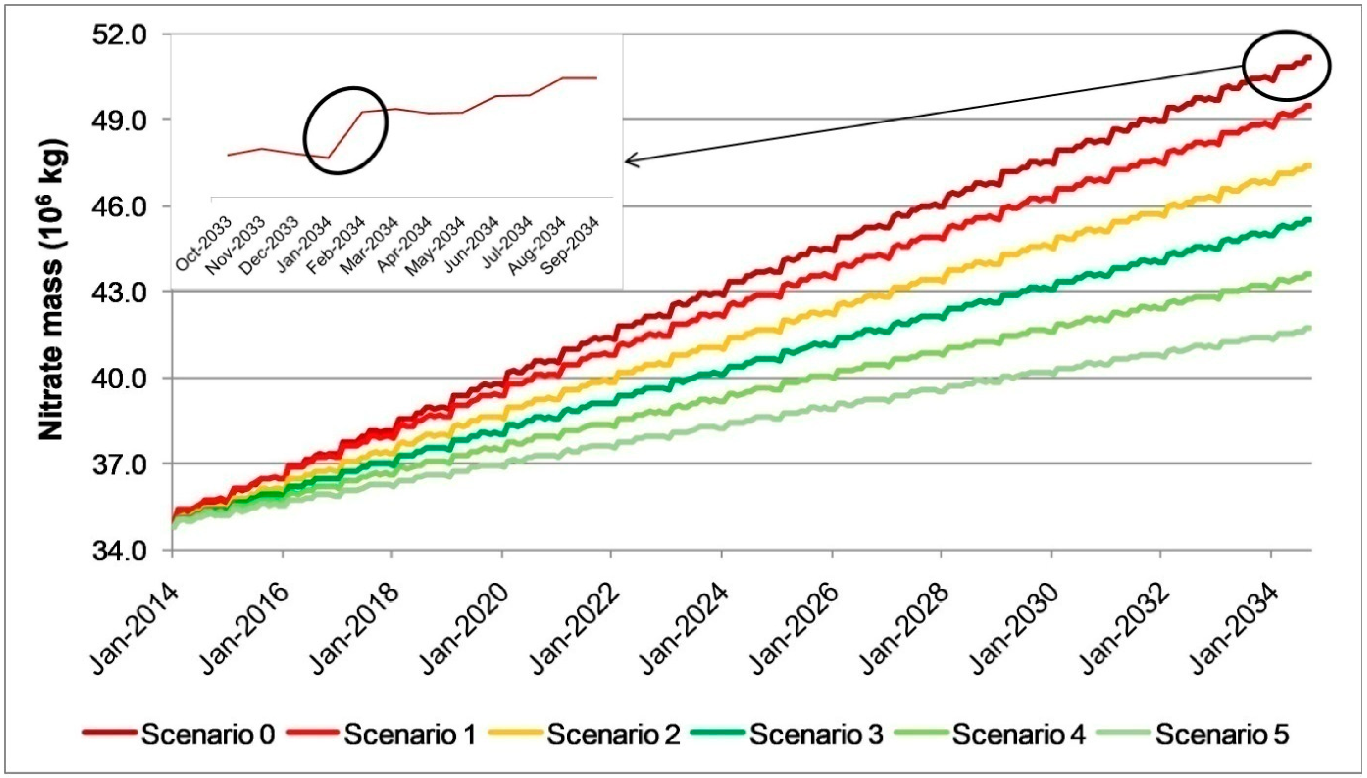
Nitrate mass: The nitrate buildup in the aquifer under study is directly derived from the numerical model, as it is a key output of the model.
-
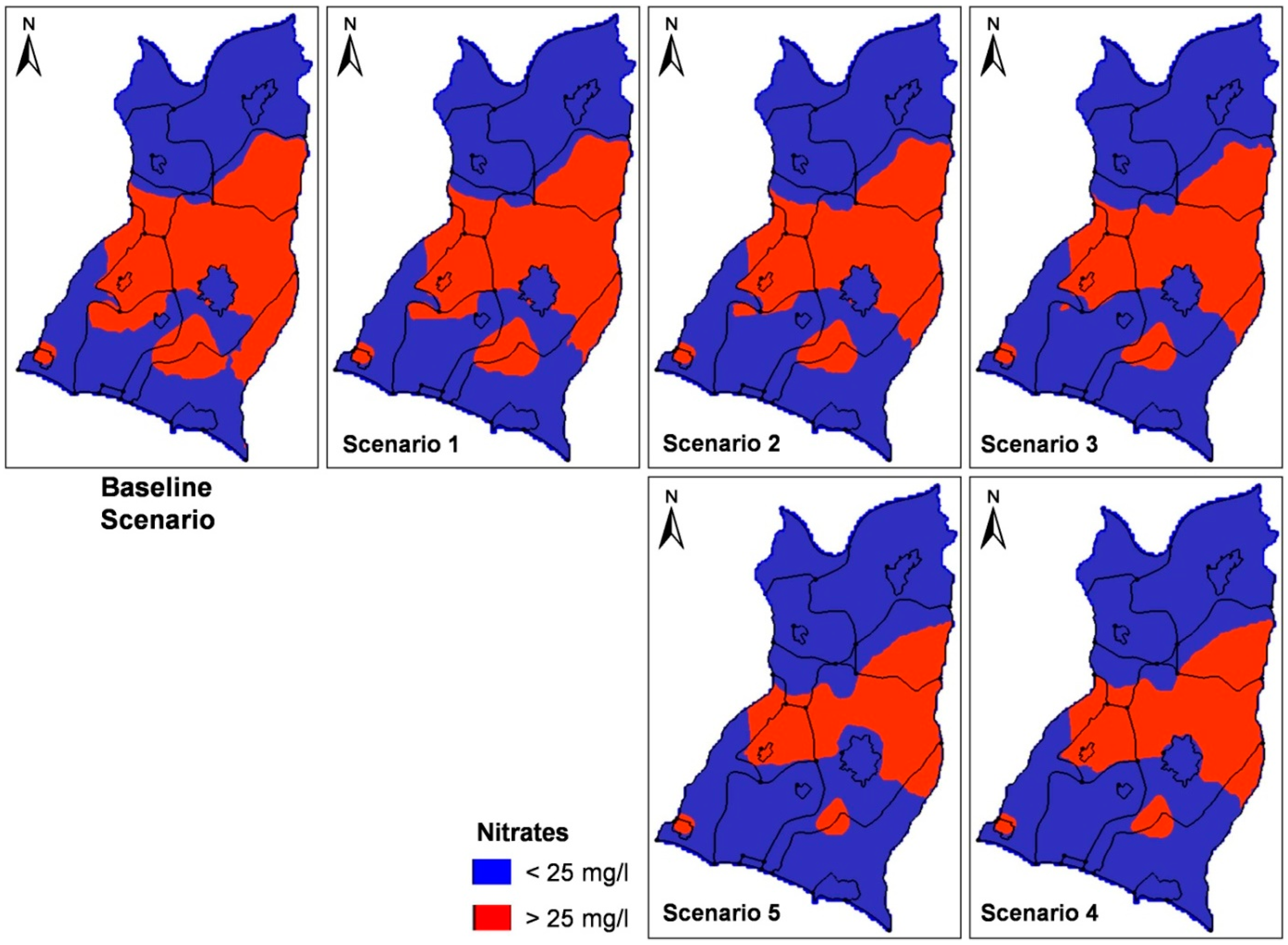
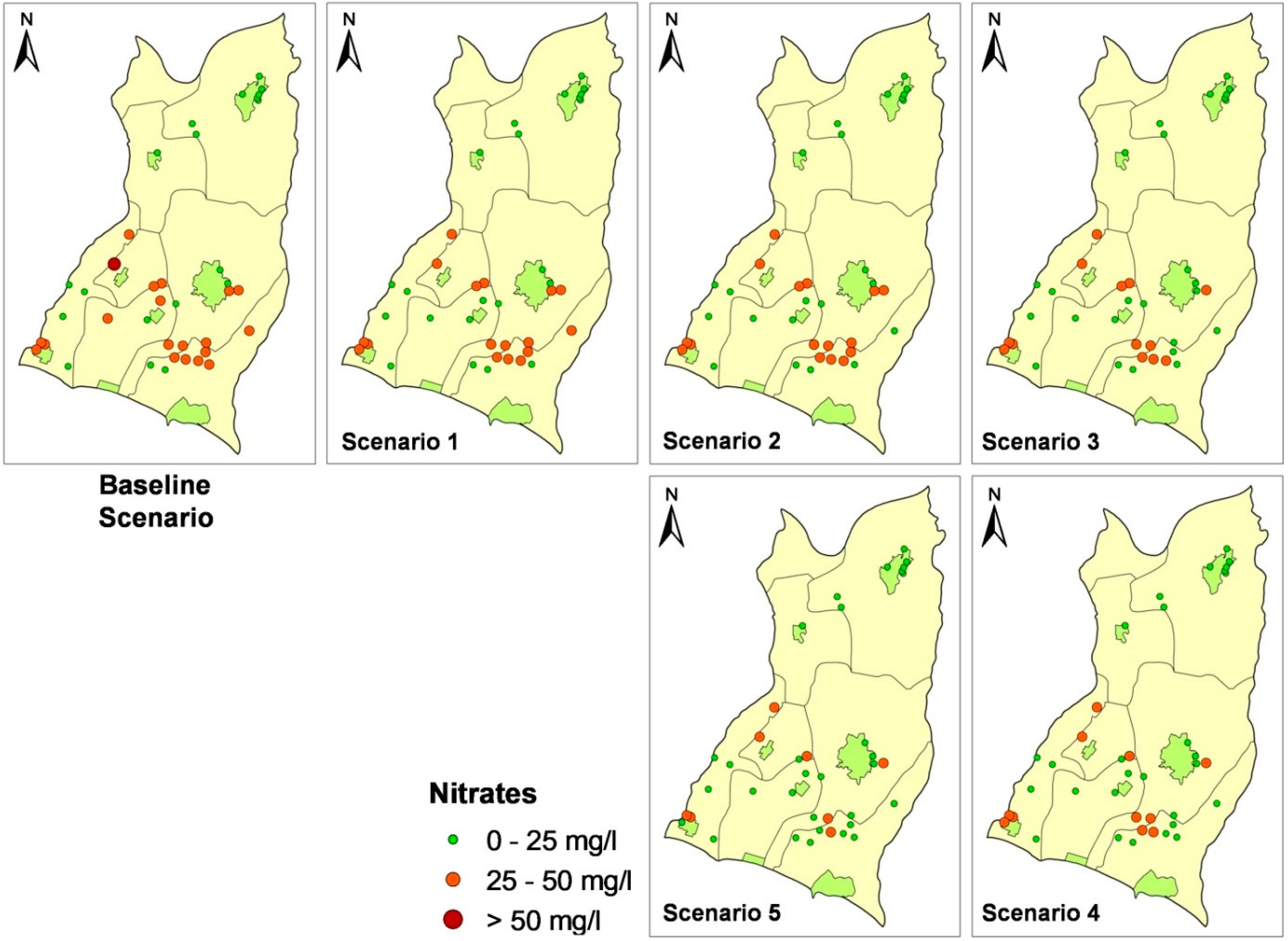
Population: The population exposed to poor-quality water refers to the total number of residents in the region supplied with water containing nitrate concentrations exceeding 25 mg/L. To determine this population for each settlement in the study area, the nitrate concentration in the water provided from the corresponding water-supply wells (see Table 1) was found. For this task, the nitrate concentration at each corresponding well (critical receptor) in every settlement was obtained from the numerical model, and then the mean concentration value (considering blended water) was computed, given that all wells in each settlement have the same pumping rate.
-
Cost: The net cost is calculated through the economic analysis as the difference in agricultural income between the do-nothing scenario and any fertilization reduction scenarios.
-
CPCR: The CPCR criterion is computed by applying the following equation:
C P C R = C O S T i A C o A C i
where COSTi is the net cost incurred from the ith scenario as previously defined, and ACo and ACi are the average nitrate concentrations at the critical receptors (water-supply wells) corresponding to the do-nothing and the ith scenario, respectively.
To evaluate the effectiveness of the different fertilization reduction scenarios according to the predefined decision criteria and select the most suitable option, the Analytic Hierarchy Process (AHP) was applied. AHP is a powerful multi-criteria decision analysis technique, frequently used for dealing with complex problems [6,73,74,75]. In this method, a series of pair-wise comparisons is set up in order to estimate the weights of the predefined decision criteria, by ranking the importance of the criteria on a scale from 1/9 (absolute unimportance) to 9 (absolute importance). A consistency ratio (CR) that measures the coherence of judgments made by decision makers is also computed. For CR ≤ 0.1, the evaluation procedure is considered acceptable; otherwise, the process should be repeated and the PCMs should be re-established [6,75,76,77]. After estimating the weights, the overall priority of each scenario (S1–S5) is calculated by summing up the results obtained by multiplying the weight of each criterion with its corresponding (normalized) value. Once the overall priorities are determined, the scenarios can be ranked, and the most appropriate one can be selected based on the highest overall priority value.

3. Results and Discussion

3.1. Numerical Modeling

In this section, the results of the nitrate fate and transport model calibration procedure are presented and discussed, as well as those referring to model application, particularly those involving the spatio-temporal variation of nitrate concentrations in the study area, along with the concentrations in water-supply wells under the various fertilizer application scenarios (S0–S5).

3.1.1. Model Calibration Results

In Figure 9, a scatterplot of the simulated versus observed nitrate concentrations for the entire set of measurements considered during the model calibration procedure is depicted, together with the values of the several evaluation measures (ME, MAE, MRSE, MRE, and R2) and the locations of the observation wells (12 wells). By considering the observed variability in nitrate concentrations, it can be inferred that the calculated errors are reasonably acceptable, indicating an overall successful calibration. Hence, the calibrated nitrate fate and transport model can be employed in order to project nitrate concentrations in response to future fertilizer application scenarios. Finally, it should be mentioned that, during the model calibration and after a series of model runs, the export coefficient for agricultural fertilizers was found to be equal to 0.42.

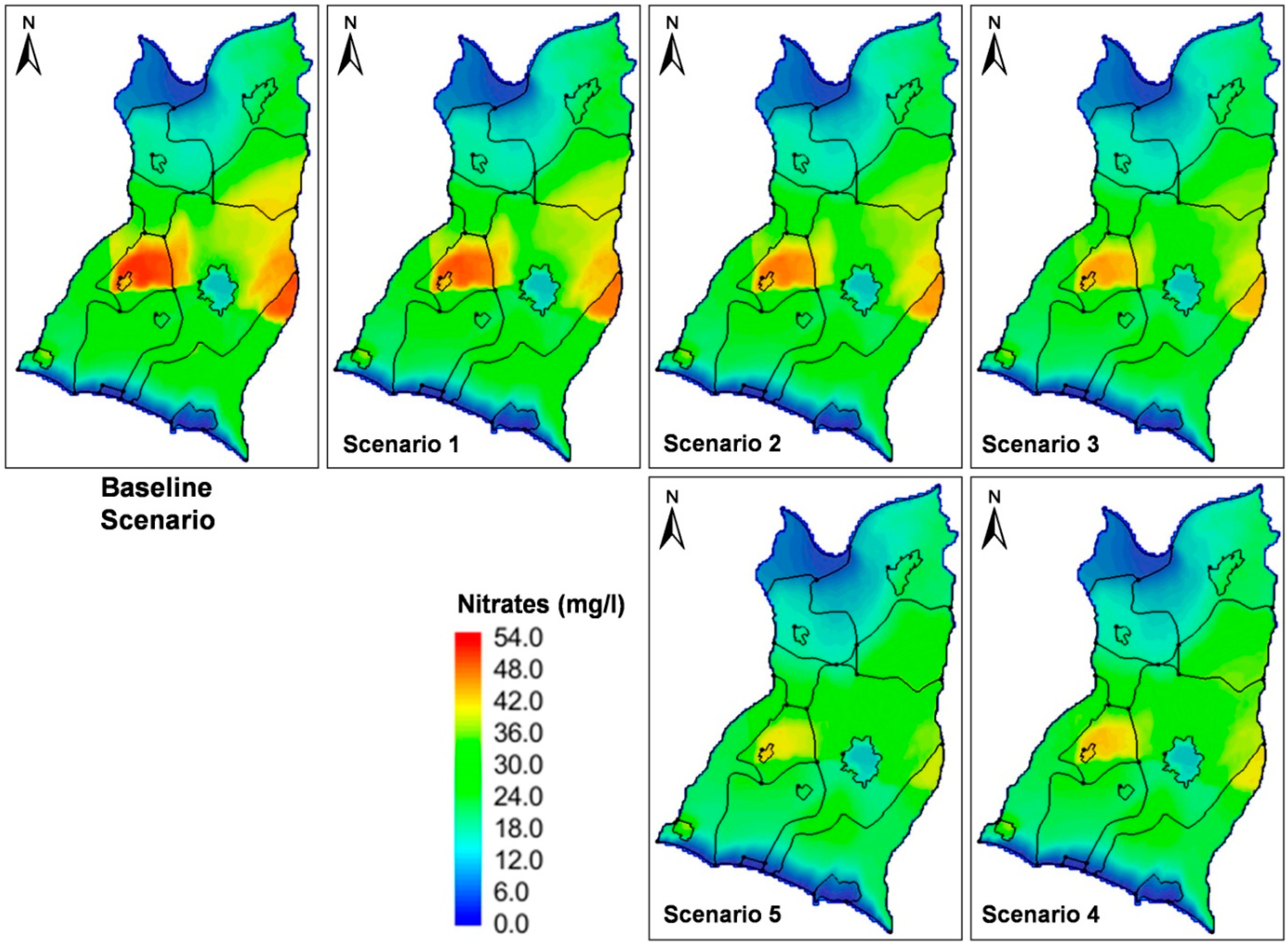
3.1.2. Model Application Results

First, the spatial distribution of nitrate concentrations for the baseline (S0) and different fertilization reduction scenarios (S1–S5) by the end of the simulation period (2034) is depicted in Figure 10. According to the modeling results, elevated nitrate concentrations exceeding the indicative threshold of 25 mg/L are mainly expected within the broader central part of the region in all considered scenarios. In particular, in Scenarios S0 and S1, nitrate levels are projected to locally surpass the upper limit of 50 mg/L. Several factors contribute to the presence of elevated concentrations within this specific area, including: (a) the combined effect of high initial nitrate concentrations in certain locations (Figure 5a) and nitrogen loading (Figure 5b) from fertilizers; (b) the direction of groundwater flow, which is towards the central part of the region (Figure 4b); and (c) the values of aquifer parameters associated with mass transport, such as the effective porosity (Table 2). Particularly regarding the latter, the lower values of effective porosity in the two central HP Zones (Figure 3a), as they were determined during the calibration/validation of the existing groundwater model (see Section 2.3.1), result in higher groundwater velocity values in that area and, therefore, in higher nitrate concentrations. In addition, elevated concentrations are anticipated in the settlement of Nea Flogita, situated in the south-western part of the region (Figure 1), due to the relatively high nitrate loading observed within it (Figure 5b) and originating from wastewater sources. On the other hand, lower nitrate concentrations are generally expected in the north-western part of the region, where both initial nitrate concentrations and nitrate loading are low (Figure 5a,b), as well as along the southern boundary of the aquifer (coastline), which was defined as a constant concentration boundary of 0 mg/L (Figure 5a) due to the intrusion of seawater from this part of the aquifer.
Furthermore, upon comparing the outcomes of the diverse fertilizer application scenarios (S0–S5), it is evident that nitrate concentrations in the region generally decrease under the fertilization reduction scenarios (S1–S5) in relation to the baseline scenario (S0). This decrease, as expected, becomes more pronounced when moving from Scenario S1 to Scenario S5, that is, to higher rates of reduction in fertilizer application (from 10% to 50%). The same conclusion can be drawn from Table 6, which presents the minimum, maximum, and mean nitrate concentrations in the region for all concerned scenarios. As is clear, the higher the reduction in fertilizer application, the lower both the maximum and mean nitrate concentrations. However, even though the mean nitrate concentration remains below the threshold of 25 mg/L in all the applied scenarios, the maximum nitrate level is above the aforementioned “guidance value” in every case; particularly in Scenarios 0 and 1, where, as previously noted, it exceeds the uppermost limit of 50 mg/L. Only when the fertilizer application rate is reduced by 20% (Scenario S2) does the maximum nitrate concentration fall below 50 mg/L.
Next, in order to distinctly localize the areas exhibiting relatively high nitrate concentrations, i.e., 25 mg/L, Figure 11 shows the spatial distribution of concentrations exceeding this threshold under various fertilizer application scenarios (S0–S5). Once again, it is apparent that, in all the scenarios considered, nitrate concentrations exceeding the “guidance value” of 25 mg/L are mainly detected within the broader central region of the study area as a result of the combined effect of initial nitrate concentrations, nitrogen loading and groundwater flow conditions. However, as the fertilizer application rate decreases (i.e., when moving from Scenario 1 to Scenario 5), the areas with concentrations above 25 mg/L tend to shrink, yet not fully diminish. This last statement implies that, despite a 50% reduction in fertilizer application, it is anticipated that nitrate concentrations above 25 mg/L will persist in a considerable part of the region, particularly concentrated in its central part.
Regarding the temporal variation in nitrates, Figure 12 displays a time-series of nitrate mass in the aquifer throughout the projection period (2014–2034) for all fertilizer application scenarios. As is clear, an increase in nitrate mass over time is observed across all scenarios. However, this increase is comparatively lower in scenarios with higher reductions in fertilizer application. Table 6 supports the same conclusion, showing an increase in both maximum and mean nitrate concentrations within the study area from 2014 to 2034 under all scenarios (nitrate concentrations are identical for all scenarios in 2014). Thus, it is clear that, regardless of the varying levels of nitrogen loading in each applied scenario, a consistent upward trend in nitrate mass over time prevails in the aquifer under study. The predominant cause of this trend generally lies in the limited nitrate discharge from the groundwater system due to the existing boundary conditions and the absence of nitrate attenuation processes, like denitrification. In addition to the overall variation in nitrate mass throughout the entire projection period, Figure 12 also shows the annual nitrate mass variation during an indicative time period (October 2023–September 2024) for Scenario 0. In this case, it is worth highlighting the substantial increase in nitrate mass during February, aligning precisely with the monthly variation in nitrogen loading in the region (Figure 7), according to which the highest levels are observed during this particular month.
In the final part of the modeling results, Figure 13 depicts the nitrate concentrations in water-supply wells for both the baseline (S0) and different fertilization reduction scenarios (S1–S5) by the end of the simulation period (2034). These findings are of great importance as they reveal the actual magnitude of nitrate contamination and the associated level of risk. They may yield valuable insights into the quality of the extracted groundwater, particularly its suitability for meeting drinking water standards. In this context, the following conclusions can be drawn: (a) none of the water-supply wells in the study area are expected to exceed the maximum allowable limit of 50 mg/L during the implementation of the fertilization reduction scenarios (S1–S5), except for one well that marginally exceeds this threshold (NO3 = 50.7 mg/L) during the baseline scenario (S0); (b) the number of water-supply wells exceeding the indicative threshold of 25 mg/L varies among the fertilization reduction scenarios (S1–S5), and specifically stands at 17 for Scenario 1, 16 for Scenario 2, 13 for Scenario 3, 11 for Scenario 4 and 9 for Scenario 5, thus rendering Scenario 5 the most effective in terms of reducing nitrate concentrations in water-supply wells; and (c) the implementation of fertilization reduction scenarios has no effect at all on the nitrate concentrations in the three water-supply wells situated near the settlement of Nea Flogita in the south-western part of the region, meaning that, in order to reduce nitrate contamination in this certain settlement, measures related to the proper management of wastewater should be considered.
However, due to the fact that a different number of water-supply wells serves each settlement (Table 1) and the water provided to each settlement is actually blended water coming from all the corresponding water-supply wells, it is important to know the nitrate concentrations in this blended water. In Table 7, the nitrate concentrations in the blended water provided by the corresponding water-supply wells to individual settlements for the different fertilization reduction scenarios (S1–S5) are presented. According to these results, it becomes evident that, as the fertilizer application decreases, there is a related reduction in the nitrate concentrations observed in the blended water, as expected. The most important conclusion, however, is associated with the number of settlements receiving blended water with nitrate concentrations exceeding the “guidance level” of 25 mg/L. This metric serves as a crucial indicator, indicating a population potentially exposed to water of inadequate quality. As it turns out, the number of settlements exceeding the 25 mg/L nitrate concentration threshold stands at three for Scenario 1, two for Scenario 2 and one for Scenarios 3, 4, and 5. It is, therefore, apparent that, even with a 50% reduction in fertilizer application, the nitrate concentrations in blended water provided to a certain settlement (the settlement of Zografou, Figure 1) are generally expected to stay above the 25 mg/L threshold.

3.2. Economic Analysis

In this section, the outcomes of the agro-economic analysis in terms of crop-yield losses in the various fertilization reduction scenarios, along with the estimated farmers’ income losses, are presented and discussed. It is important, however, to mention that only the three principal crops—wheat, olives, and apricots—detected in the study area were included in the analysis, since these crops, as already mentioned, comprise 96% of the total cultivated land in the region. Therefore, the decrease in the farmers’ income resulting from the reduced production of the aforementioned crops quite accurately reflects the total income loss in the region associated with agricultural activities.
First, in Table 8, the agro-economic data related to the three crops considered in the analysis, and required in order to apply Equation (1) in estimating the crop-yield losses resulting from the reduced fertilizer usage (see Section 3.2), are given. Next, Table 9 presents the estimated crop-yield losses for each crop and fertilization reduction scenario (S1–S5) in both net absolute values and percentages (in parentheses). The results indicate that fertilizer reduction has, in general, a greater impact on wheat (considering the percentage reduction in crop-yield), which is mainly attributable to the smaller variations between the expected crop-yield (3500 kg/ha) and the yield with no nutrient applied (1750 kg/ha) as compared to the other two crops.
Subsequently, the results of the economic analysis in terms of farmers’ income losses due to fertilizer restrictions are presented. However, to obtain these results, the farmers’ income for the baseline (S0) and fertilization reduction scenarios (S1–S5) were initially calculated. For this task, the revenue generated by farmers and the costs associated with crop production were considered, and the latter was subtracted from the former. Farmers’ revenues were calculated by multiplying the total crop production by the respective selling price. Alternatively, production costs were calculated by summing the expenses incurred for labor, involving the costs associated with both human and machinery hours, together with material expenses, including seeds, fertilizers, and pesticides. In Table 10, the results derived from the aforementioned procedure for each type of crop considered in the analysis, namely wheat, olives and apricots, in the case of the baseline scenario (S0), are provided. From these findings, it is clear that olives play a substantial role in the total farmers’ income in the region, making up roughly 66% of the overall income, followed by apricots, with a contribution of about 31%.
The same process as above was applied consistently across all fertilization reduction scenarios (S1–S5), with adjustments solely focused on the crop yield (referred to as “b”), as indicated by the values presented in Table 9, and fertilizer costs (referred to as “g”). In Table 11, the estimated farmers’ income losses for each crop, together with the total income losses resulting from the implementation of different fertilization reduction scenarios (S1–S5), are presented. It is evident that the higher the reduction in fertilizer application, the higher the economic losses for each crop. Specifically, olive productions suffer the greatest loss of annual income in net absolute terms, ranging from 381,943 EUR in Scenario 1 (10% reduction in fertilizer application) to 5,703,246 EUR in Scenario 5 (50% reduction in fertilizer application). In the case of the most economically adverse scenario, i.e., Scenario 5, wheat indicates a loss of 400,535 EUR, while apricots show a loss of 2,301,839 EUR, culminating in a total income reduction of 8,405,620 EUR across all three crops. To provide a clearer insight into the economic impact of fertilization restrictions on individual crops, Figure 14 shows the percentage decrease in yearly earnings for each crop under various fertilization reduction scenarios. Among all three crops, wheat exhibits the greatest percentage income reduction, notably a 21.4% decrease with a 50% reduction in fertilizer usage (Scenario 5). Olives and apricots, on the other hand, demonstrate income reductions of 16.0% and 13.8%, respectively, under the same scenario.

3.3. Decision Analysis

In this section, the results of the decision analysis procedure regarding the estimation of decision criteria weights, along with scenarios ranking, are presented and discussed. First, in Table 12, a pair-wise comparison matrix for the four decision criteria considered in the analysis, as determined based on the importance order of criteria, is provided, along with the estimated criteria weights. It is worthwhile to mention that, among the selected criteria, the highest preference (greatest importance) was placed on the criterion referring to the population at risk, considering that the primary objective of the management measures, i.e., the fertilization reduction scenarios, is safeguarding public health. Regarding the remaining criteria, the order is as follows: CPCR, cost and nitrate mass.
Next, Table 13 displays the values calculated for all decision criteria in each fertilization reduction scenario (S1–S5) as determined through the nitrate fate and transport model and the economic analysis, in addition to the corresponding scenario rankings. At this point, it should be mentioned that the ranking scores, as shown at the last column of Table 13, were computed following the normalization of the values of the selected criteria. According to the results, it can be evidently concluded that Scenario 3, entailing a 30% reduction in fertilizer application, is superior to all other scenarios, thus standing out as the most favorable option for the area under study, considering both the environmental and economic perspectives. The performance of this alternative scenario, particularly when compared to Scenarios 4 and 5 which encompass higher reductions in fertilizer application, is primarily attributed to the consistency across all the aforementioned scenarios in terms of the population exposed to water with nitrate concentrations exceeding the “guidance value” of 25 mg/L. Under these conditions, and given the fact that both net cost and CPCR increase in the case of Scenarios 4 and 5, the ranking score of Scenario 3 turns out to be higher than that of the other scenarios. However, Scenario 4 claimed the second position following Scenario 3, while Scenario 5 achieved the third place in the ranking scheme. As far as the remaining scenarios are concerned, despite a larger population being exposed to poor-quality water in Scenario 1, it outperforms Scenario 2 due to the lower net cost and CPCR value.
At this point, it is worthwhile to mention that these findings, and particularly the designation of Scenario3 as the most recommendable option for the study area, seem to offer a rather “stable” solution, with minimal susceptibility to uncertainties linked to certain problem parameters, such as the “export coefficient” used for calculating nitrate leaching. This is mainly attributable to both the assumptions made during the formulation of the numerical model (involving conservative, advective-dispersive transport for the nitrates) and the model outcomes concerning nitrate concentrations in the blended water provided to the various settlements in the study area (see Table 7).
In conclusion, it can be inferred that, considering both environmental and economic aspects, a moderate reduction in fertilizer application (Scenario 3) was found to be the most suitable solution for the area under study. Even though higher reductions in fertilizers lead to a greater decrease in nitrate concentrations in the local groundwater resources, it appears that these reductions do not actually have a direct impact on the population exposed to poor-quality water. Conversely, higher reductions result in greater economic ramifications for farmers without actually offering a more effective solution regarding the quality of water provided to the residents of a certain settlement in the study area, since nitrate concentrations in drinking water remain above 25 mg/L. Under these conditions, with a portion of the local population in the study area still at risk, it becomes evident that, despite the implementation of fertilization restrictions, they alone do not offer an absolute solution in an effort to comply with drinking water standards. In this context, it is important to explore a more holistic management approach that integrates fertilizer regulations with more thorough strategies (i.e., abandoning existing wells with nitrate concentrations above 25 mg/L and constructing new ones within the potentially non-contaminated part of the aquifer). However, the solution identified through the proposed framework can serve as a foundation and be combined with additional measures with the ultimate goal of ensuring complete public health safety in the study area.

4. Conclusions

In the present study, an integrated framework aimed at properly managing groundwater nitrate contamination resulting from the excessive use of fertilizers in rural areas was developed. Specifically, the framework attempts to investigate and evaluate the implementation of fertilization restriction policies by considering both environmental and economic aspects in an effort to identify and propose the most appropriate option. To achieve this, numerical modeling was applied to study the spatio-temporal variation of nitrate concentrations, while an agro-economic analysis was performed to assess the economic impact of fertilization restrictions. As a final step, a multi-criteria decision analysis was carried out, incorporating criteria associated with both the environmental and economic assessment of fertilizer regulations, while placing specific emphasis on ensuring the quality of water provided to local population (i.e., reducing health risks). To test the methodology, five different scenarios, in which fertilizer application was reduced by certain rates (10%, 20%, 30%, 40% and 50%), were formed, evaluated and ranked.
The case study implementation revealed that, even though a 50% reduction in fertilizers resulted in lower nitrate concentrations in local groundwater resources, this option did not emerge as the most favorable one when considering all the criteria examined. Instead, a 30% reduction was identified as the most efficient solution specifically designated for the area being studied (site-specific finding), as it not only carries a similar level of risk to local residents compared to scenarios with higher reduction rates, but also leads to reduced economic losses for farmers. It then becomes clear that implementing such an approach is crucial when faced with selecting the most appropriate option among alternatives with conflicting objectives. Within this context, the proposed framework could serve as a useful and practical set of guidelines in designing efficient fertilizer regulation policies that consider both environmental and economic perspectives, considerably contributing to the proper management of nitrate contamination caused by agricultural fertilizers in rural areas. It might also provide valuable insights for conducting a more comprehensive management of nitrate contamination, particularly in cases where fertilizer restrictions fall short of fully guaranteeing water quality.
However, in order to expand the applicability of the proposed framework, future research could extend its analysis beyond fertilizer restrictions, encompassing additional policies which could implemented to control groundwater nitrate contamination. Such policies could either include different mechanisms for reducing fertilizer application, such as pricing policies (e.g., taxes) and changes in land use (e.g., from croplands to grassland or forest), or focus on addressing other potential sources of nitrate contamination, such as manure application, animal feedlot operations and urban wastewater sources (e.g., septic systems). In this context, additional criteria associated with the societal costs resulting from reductions in crop productivity could be considered in the decision-making process, thus leading to a more holistic evaluation of the impacts of fertilizer regulations. Additional work might also involve an all-inclusive analysis of the modeling system on the basis of the “Origin (land surface)—Pathway (vadose zone)—Target (aquifer)” model, thus allowing for a more detailed calculation of on-ground nitrogen loading (e.g., on a farm level) to be conducted, while also modeling nitrogen dynamics in the unsaturated zone. Finally, an update to the nitrate fate and transport model presented in the current study should be considered, specifically involving a more rigorous model validation, using new datasets of nitrate measurements from the area being studied.

Author Contributions

Conceptualization, I.S.; methodology, I.S. and Z.M.; software, I.S.; validation, I.S.; formal analysis, I.S.; investigation, I.S.; resources, I.S.; writing—original draft preparation, I.S. and Z.M.; writing—review and editing, I.S., Z.M. and P.L.; visualization, I.S.; supervision, P.L. All authors have read and agreed to the published version of the manuscript.

Funding

This research received no external funding.

Data Availability Statement

The data used in this study are contained within the article. Additional data are available upon request from the corresponding author.

Acknowledgments

Part of the research was conducted by Ilias Siarkos as a PHD candidate at the School of Civil Engineering, Aristotle University of Thessaloniki, Thessaloniki, Greece. Moreover, the authors would particularly like to thank Stefanos Sevastas for his assistance in acquiring the necessary agro-economic data used in the economic analysis.

Conflicts of Interest

The authors declare no conflict of interest.

References

  1. De Filippis, G.; Ercoli, L.; Rossetto, R. A spatially distributed, physically-based modeling approach for estimating agricultural nitrate leaching to groundwater. Hydrology 2021, 8, 8. [Google Scholar] [CrossRef]
  2. Mirzaee, M.; Safavi, H.R.; Taheriyoun, M.; Rezaei, F. Multi-objective optimization for optimal extraction of groundwater from a nitrate-contaminated aquifer considering economic-environmental issues: A case study. J. Contam. Hydrol. 2021, 241, 103806. [Google Scholar] [CrossRef]
  3. Shultz, C.D.; Gates, T.K.; Bailey, R.T. Evaluating best management practices to lower selenium and nitrate in groundwater and streams in an irrigated river valley using a calibrated fate and reactive transport model. J. Hydrol. 2018, 566, 299–312. [Google Scholar] [CrossRef]
  4. Sishu, F.K.; Tilahun, S.A.; Schmitter, P.; Steenhuis, T.S. Investigating nitrate with other constituents in groundwater in two contrasting tropical highland watersheds. Hydrology 2023, 10, 82. [Google Scholar] [CrossRef]
  5. Wei, X.; Bailey, R.T.; Records, R.M.; Wible, T.G.; Arabi, M. Comprehensive simulation of nitrate transport in coupled surface-subsurface hydrologic systems using the linked SWAT-MODFLOW-RT3D model. Environ. Modell. Softw. 2019, 122, 104242. [Google Scholar] [CrossRef]
  6. Almasri, M.N. Nitrate contamination of groundwater: A conceptual management framework. Environ. Impact Asses. 2007, 27, 220–242. [Google Scholar] [CrossRef]
  7. Ji, W.; Xiao, J.; Toor, G.S.; Li, Z. Nitrate-nitrogen transport in streamwater and groundwater in a loess covered region: Sources, drivers, and spatiotemporal variation. Sci. Total Environ. 2021, 761, 143278. [Google Scholar] [CrossRef]
  8. Latinopoulos, P. Nitrate contamination of groundwater: Modeling as a tool for risk assessment, management and control. In Groundwater Pollution Control; Katsifarakis, K.L., Ed.; WIT Press: Southampton, UK, 1999; pp. 1–48. [Google Scholar]
  9. Sullivan, T.P.; Gao, Y.; Reimann, T. Nitrate transport in a karst aquifer: Numerical model development and source evaluation. J. Hydrol. 2019, 573, 432–448. [Google Scholar] [CrossRef]
  10. Viers, J.H.; Liptzin, D.; Rosenstock, T.S.; Jensen, V.B.; Hollander, A.D.; McNally, A.; King, A.M.; Kourakos, G.; Lopez, E.M.; De La Mora, N.; et al. Nitrogen sources and loading to groundwater. In Addressing Nitrate in California’s Drinking Water with a Focus on Tulare Lake Basin and Salinas Valley Groundwater; Technical Report 2; University of California: Davis, CA, USA, 2012. [Google Scholar]
  11. Buskulic, P.; Parlov, J.; Kovac, Z.; Nakic, Z. Estimation of nitrate background value in groundwater under the long-term human impact. Hydrology 2023, 10, 63. [Google Scholar] [CrossRef]
  12. Sidiropoulos, P.; Mylopoulos, N.; Vasiliades, L.; Loukas, A. Stochastic nitrate simulation under hydraulic conductivity uncertainty of an agricultural basin aquifer at Eastern Thessaly, Greece. Environ. Sci. Pollut. R. 2021, 28, 65700–65715. [Google Scholar] [CrossRef]
  13. Wick, K.; Heumesser, C.; Schmid, E. Groundwater nitrate contamination: Factors and indicators. J. Environ. Manag. 2012, 111, 178–186. [Google Scholar] [CrossRef]
  14. Zhang, H.; Yang, R.; Wang, Y.; Ye, R. The evaluation and prediction of agriculture-related nitrate contamination in groundwater in Chengdu Plain, southwestern China. Hydrogeol. J. 2019, 27, 785–799. [Google Scholar] [CrossRef]
  15. Ameur, M.; Aouiti, S.; Hamzaoui-Azaza, F.; Cheikha, L.B.; Gueddari, M. Vulnerability assessment, transport modeling and simulation of nitrate in groundwater using SI method and modflow-MT3DMS software: Case of Sminja aquifer, Tunisia. Environ. Earth Sci. 2021, 80, 220. [Google Scholar] [CrossRef]
  16. Correa-Gonzalez, A.; Hernandez-Bedolla, J.; Martinez-Cinco, M.A.; Sanchez-Quispe, S.T.; Hernandez-Hernandez, M.A. Assessment of nitrate in groundwater from diffuse sources considering spatiotemporal patterns of hydrological systems using a coupled SWAT/MODFLOW/MT3DMS model. Hydrology 2023, 10, 209. [Google Scholar] [CrossRef]
  17. Almasri, M.N.; Kaluarachchi, J.J. Modeling nitrate contamination of groundwater in agricultural watersheds. J. Hydrol. 2007, 343, 211–229. [Google Scholar] [CrossRef]
  18. Bryan, N.S.; Van Grinsven, H. The role of nitrate in human health. Adv. Agron. 2013, 119, 153–182. [Google Scholar]
  19. Sidiropoulos, P.; Tziatzios, G.; Vasiliades, L.; Mylopoulos, N.; Loukas, A. Groundwater nitrate contamination integrated modeling for climate and water resources scenarios: The case of Lake Karla over-exploited aquifer. Water 2019, 11, 1201. [Google Scholar] [CrossRef]
  20. Wolfe, A.H.; Patz, J.A. Reactive nitrogen and human health: Acute and long-term implications. Ambio 2002, 31, 120–125. [Google Scholar] [CrossRef]
  21. Powlson, D.S.; Addiscott, T.M.; Benjamin, N.; Cassman, K.G.; De Kok, T.M.; Van Grinsven, H.; L’hirondel, J.; Avery, A.A.; Van Kessel, C. When does nitrate become a risk for humans? J. Environ. Qual. 2008, 37, 291–295. [Google Scholar] [CrossRef]
  22. Zhang, F.-X.; Miao, Y.; Ruan, J.-G.; Meng, S.-P.; Dong, J.-D.; Yin, H.; Huang, Y.; Chen, F.-R.; Wang, Z.-C.; Lai, Y.-F. Association between nitrite and nitrate intake and risk of gastric cancer: A systematic review and meta-analysis. Med. Sci. Monit. 2019, 25, 1788–1799. [Google Scholar] [CrossRef]
  23. Xin, J.; Wang, Y.; Shen, Z.; Liu, Y.; Wang, H.; Zheng, X. Critical review of measures and decision support tools for groundwater nitrate management: A surface-to-groundwater profile perspective. J. Hydrol. 2021, 598, 126386. [Google Scholar] [CrossRef]
  24. Bastani, M.; Harter, T. Source area management practices as remediation tool to address groundwater nitrate pollution in drinking supply wells. J. Contam. Hydrol. 2019, 226, 103521. [Google Scholar] [CrossRef]
  25. Pena-Haro, S.; Pulido-Velazquez, M.; Sahuquillo, A. A hydro-economic modelling framework for optimal management of groundwater nitrate pollution from agriculture. J. Hydrol. 2009, 373, 193–203. [Google Scholar] [CrossRef]
  26. Kumar, P.; Thakur, P.K.; Bansod, B.K.S.; Debnath, S.K. Groundwater: A regional resource and a regional governance. Environ. Dev. Sustain. 2018, 20, 1133–1151. [Google Scholar] [CrossRef]
  27. Siarkos, I.; Sevastas, S.; Latinopoulos, D. Using a hydroeconomic model to evaluate alternative methods applied for the delineation of protection zones. Desalin. Water. Treat. 2018, 133, 315–326. [Google Scholar] [CrossRef]
  28. Siarkos, I.; Arfaoui, M.; Tzoraki, O.; Zammouri, M.; Hamzaoui-Azaza, F. Implementation and evaluation of different techniques to modify DRASTIC method for groundwater vulnerability assessment: A case study from Bouficha aquifer, Tunisia. Environ. Sci. Pollut. Res. 2023, 30, 89459–89478. [Google Scholar] [CrossRef]
  29. Almasri, M.N.; Kaluarachchi, J.J. Multi-criteria decision analysis for the optimal management of nitrate contamination of aquifers. J. Environ. Manag. 2005, 74, 365–381. [Google Scholar] [CrossRef]
  30. Liu, R.; Zhang, P.; Wang, X.; Chen, Y.; Shen, Z. Assessment of effects of best management practices on agricultural non-point source pollution in Xiangxi River watershed. Agric. Water Manag. 2013, 117, 9–18. [Google Scholar] [CrossRef]
  31. Samadi-Darafshani, M.; Safavi, H.R.; Golmohammadi, M.H.; Rezaei, F. Assessment of the management scenarios for groundwater quality remediation of a nitrate-contaminated aquifer. Environ. Monit. Assess. 2021, 193, 190. [Google Scholar] [CrossRef]
  32. Yang, L.; Zheng, C.; Andrews, C.B.; Wang, C. Applying a regional transport modeling framework to manage nitrate contamination of groundwater. Groundwater 2021, 59, 292–307. [Google Scholar] [CrossRef]
  33. Almasri, M.N.; Kaluarachchi, J.J. Assessment and management of long-term nitrate pollution of ground water in agriculture-dominated watersheds. J. Hydrol. 2004, 295, 225–245. [Google Scholar] [CrossRef]
  34. Reed, E.M.; Wang, D.; Duranceau, S.J. Evaluating nitrate management in the Volusia Blue Springshed. J. Environ. Eng. 2018, 144, 05018001. [Google Scholar] [CrossRef]
  35. Karlovic, I.; Posavec, K.; Larva, O.; Markovic, T. Numerical groundwater flow and nitrate transport assessment in alluvial aquifer of Varazdin region, NW Croatia. J. Hydrol. Reg. Stud. 2022, 41, 101084. [Google Scholar] [CrossRef]
  36. Musacchio, A.; Mas-Pla, J.; Soana, E.; Re, V.; Sacchi, E. Governance and groundwater modelling: Hints to boost the implementation of the EU Nitrate Directive. The Lombardy Plain case, N Italy. Sci. Total Environ. 2021, 782, 146800. [Google Scholar] [CrossRef]
  37. Rawat, M.; Sen, R.; Onyekwelu, I.; Wiederstein, T.; Sharda, V. Modeling of groundwater nitrate contamination due to agricultural activities—A systematic review. Water 2022, 14, 4008. [Google Scholar] [CrossRef]
  38. Zhang, H.; Yang, R.; Guo, S.; Li, Q. Modeling fertilization impacts on nitrate leaching and groundwater contamination with HYDRUS-1D and MT3DMS. Paddy Water Environ. 2020, 18, 481–498. [Google Scholar] [CrossRef]
  39. Hou, C.; Chu, M.L.; Botero-Acosta, A.; Guzman, J.A. Modeling field scale nitrogen non-point source pollution (NPS) fate and transport: Influences from land management practices and climate. Sci. Total Environ. 2021, 759, 143502. [Google Scholar] [CrossRef]
  40. Zhang, H.; Hiscock, K.M. Modelling the effect of forest cover in mitigating nitrate contamination of groundwater: A case study of the Sherwood Sandstone aquifer in the East Midlands, UK. J. Hydrol. 2011, 399, 212–225. [Google Scholar] [CrossRef]
  41. Gomann, H.; Kreins, P.; Kunkel, R.; Wendland, F. Model based impact analysis of policy options aiming at reducing diffuse pollution by agriculture—A case study for the river Ems and a sub-catchment of the Rhine. Environ. Modell. Softw. 2005, 20, 261–271. [Google Scholar] [CrossRef]
  42. Graveline, N.; Rinaudo, J.D.; Segger, V.; Lambrecht, H.; Casper, M.; Elsass, P.; Grimm-Strele, J.; Gudera, T.; Koller, R.; Van Dijk, P. Integrating economic and groundwater models for developing long-term nitrate concentration scenarios in a large aquifer. In Aquifer Systems Management: Darcy’s Legacy in a World of Impending Water Shortage; Chery, L., Marsily, G., Eds.; Taylor & Francis: New York, NY, USA, 2007; pp. 483–495. [Google Scholar]
  43. Pena-Haro, S.; Llopis-Albert, C.; Pulido-Velazquez, M.; Pulido-Velazquez, D. Fertilizer standards for controlling groundwater nitrate pollution from agriculture: El Salobral-Los Llanos case study, Spain. J. Hydrol. 2010, 392, 174–187. [Google Scholar] [CrossRef]
  44. Liu, G.; Chen, L.; Wei, G.; Shen, Z. New framework for optimizing best management practices at multiple scales. J. Hydrol. 2019, 578, 124133. [Google Scholar] [CrossRef]
  45. Dotoli, M.; Epicoco, N.; Falagario, M. Multi-criteria decision making techniques for the management of public procurement tenders: A case study. Appl. Soft. Comput. 2020, 88, 106064. [Google Scholar] [CrossRef]
  46. Latinopoulos, P. Development of water resources management plan for water supply and irrigation. In Final Report Prepared for: Municipality of Nea Moudania; Aristotle University of Thessaloniki: Thessaloniki, Greece, 2003. (In Greek) [Google Scholar]
  47. Syridis, G. Lithostromatographical, Biostromatographical and Paleostromatographical Study of Neogene-Quaternary Formation of Chalkidiki Peninsula. Ph.D. Thesis, Aristotle University of Thessaloniki, Thessaloniki, Greece, 1990. (In Greek). [Google Scholar]
  48. Siarkos, I. Developing a Methodological Framework Using Mathematical Simulation Models in Order to Investigate the Operation of Coastal Aquifer Systems: Application in the Aquifer of Nea Moudania. Ph.D. Thesis, Aristotle University of Thessaloniki, Thessaloniki, Greece, 2015. (In Greek). [Google Scholar]
  49. Siarkos, I.; Latinopoulos, P. Modeling seawater intrusion in overexploited aquifers in the absence of sufficient data: Application to the aquifer of Nea Moudania, northern Greece. Hydrogeol. J. 2016, 24, 2123–2141. [Google Scholar] [CrossRef]
  50. Shamrukh, M.; Corapcioglu, M.Y.; Hassona, F.A.A. Modeling the effect of chemical fertilizers on ground water quality in the Nile Valley aquifer, Egypt. Groundwater 2001, 39, 59–67. [Google Scholar] [CrossRef]
  51. Siarkos, I.; Latinopoulos, D.; Mallios, Z.; Latinopoulos, P. A methodological framework to assess the environmental and economic effects of injection barriers against seawater intrusion. J. Environ. Manag. 2017, 193, 532–540. [Google Scholar] [CrossRef] [PubMed]
  52. Guo, W.; Langevin, C.D. User’s guide to SEAWAT: A computer program for simulation of three-dimensional variable-density groundwater flow. In Techniques of Water-Resources Investigations, Book 6-A7; USGS: Reston, VA, USA, 2002. [Google Scholar]
  53. Zheng, C.; Wang, P.P. MT3DMS: A Modular Three-Dimensional Multispecies Transport Model for Simulation of Advection, Dispersion, and Chemical Reactions of Contaminants in Groundwater Systems—Documentation and User’s Guide; Contract Report SERD-99-1; US Army Corps of Engineers: Washington, DC, USA, 1999.
  54. Almasri, M.N.; Kaluarachchi, J.J. Implications of on-ground nitrogen loading and soil transformations on ground water quality management. J. Am. Water Resour. Assoc. 2004, 40, 165–186. [Google Scholar] [CrossRef]
  55. Hajhamad, L.; Almasri, M.N. Assessment of nitrate contamination of groundwater using lumped-parameter models. Environ. Modell. Softw. 2009, 24, 1073–1087. [Google Scholar] [CrossRef]
  56. Kaluarachchi, J.; Almasri, M. Conceptual Model of Fate and Transport of Nitrate in the Extended Sumas-Blaine Aquifer, Whatcom County, Washington; Project Report; Utah State University: Logan, UT, USA, 2002. [Google Scholar]
  57. Ministry of Rural Development and Food. Data on the Integrated Management System of Cultivated Areas; Ministry of Rural Development and Food: Athens, Greece, 2007.
  58. Zhang, J.; Jorgensen, S.E. Modelling of point and non-point nutrient loadings from a watershed. Environ. Modell. Softw. 2005, 20, 561–574. [Google Scholar] [CrossRef]
  59. ASAE. Manure Production and Characteristics; D384.2; American Society of Agricultural Engineers: St. Joseph, MI, USA, 2005. [Google Scholar]
  60. Meisinger, J.J.; Randall, G.W. Estimating nitrogen budgets for soil-crop systems. In Managing Nitrogen for Groundwater Quality and Farm Profitability; Follet, R.F., Keeney, D.R., Cruse, R.M., Eds.; Soil Science Society of America: Madison, WI, USA, 1991; pp. 85–124. [Google Scholar]
  61. Cox, S.E.; Kahle, S.C. Hydrogeology, Ground-Water Quality, and Sources of Nitrate in Lowland Glacial Aquifers of Whatcom County, Washington, and British Columbia, Canada; Water-Resources Investigations Report 98-4195; U.S. Geological Survey: Reston, VA, USA, 1999.
  62. Zhang, H.; Hiscock, K.M. Modelling response of groundwater nitrate concentration in public supply wells to land-use change. Q. J. Eng. Geol. Hydrog. 2016, 49, 170–182. [Google Scholar] [CrossRef]
  63. Peterson, E.W.; Hayden, K.M. Transport and fate of nitrate in the streambed of a low-gradient stream. Hydrology 2018, 5, 55. [Google Scholar] [CrossRef]
  64. Puig, R.; Soler, A.; Widory, D.; Mas-Pla, J.; Domenech, C.; Otero, N. Characterizing sources and natural attenuation of nitrate contamination in the Baix Ter aquifer system (NE Spain) using a multi-isotope approach. Sci. Total Environ. 2017, 580, 518–532. [Google Scholar] [CrossRef] [PubMed]
  65. Eryigit, M.; Engel, B. Spatiotemporal modelling of groundwater flow and nitrate contamination in an agriculture-dominated watershed. J. Environ. Inform. 2022, 39, 125–135. [Google Scholar] [CrossRef]
  66. Kourgialas, N.N.; Karatzas, G.P.; Koubouris, G.C. A GIS policy approach for assessing the effect of fertilizers on the quality of drinking and irrigation water and wellhead protection zones (Crete, Greece). J. Environ. Manag. 2017, 189, 150–159. [Google Scholar] [CrossRef] [PubMed]
  67. Xefteris, A.; Anastasiadis, P.; Latinopoulos, P. Groundwater chemical characteristics in Kalamaria Plain, Halkidiki Peninsula, Greece. Fresen. Environ. Bull. 2004, 13, 1158–1167. [Google Scholar]
  68. Rivett, M.O.; Buss, S.R.; Morgan, P.; Smith, J.W.N.; Bemment, C.D. Nitrate attenuation in groundwater: A review of biogeochemical controlling processes. Water Res. 2008, 42, 4215–4232. [Google Scholar] [CrossRef] [PubMed]
  69. Tesoriero, A.; Liecscher, S.; Cox, S. Mechanism and rate of denitrification in an agricultural watershed: Electron and mass balance along ground water flow paths. Water Resour. Res. 2000, 36, 1545–1559. [Google Scholar] [CrossRef]
  70. Psarropoulou, E.T.; Karatzas, G.P. Pollution of nitrates—Contaminant transport in heterogeneous porous media: A case study of the coastal aquifer of Corinth, Greece. Global Nest J. 2014, 16, 9–23. [Google Scholar]
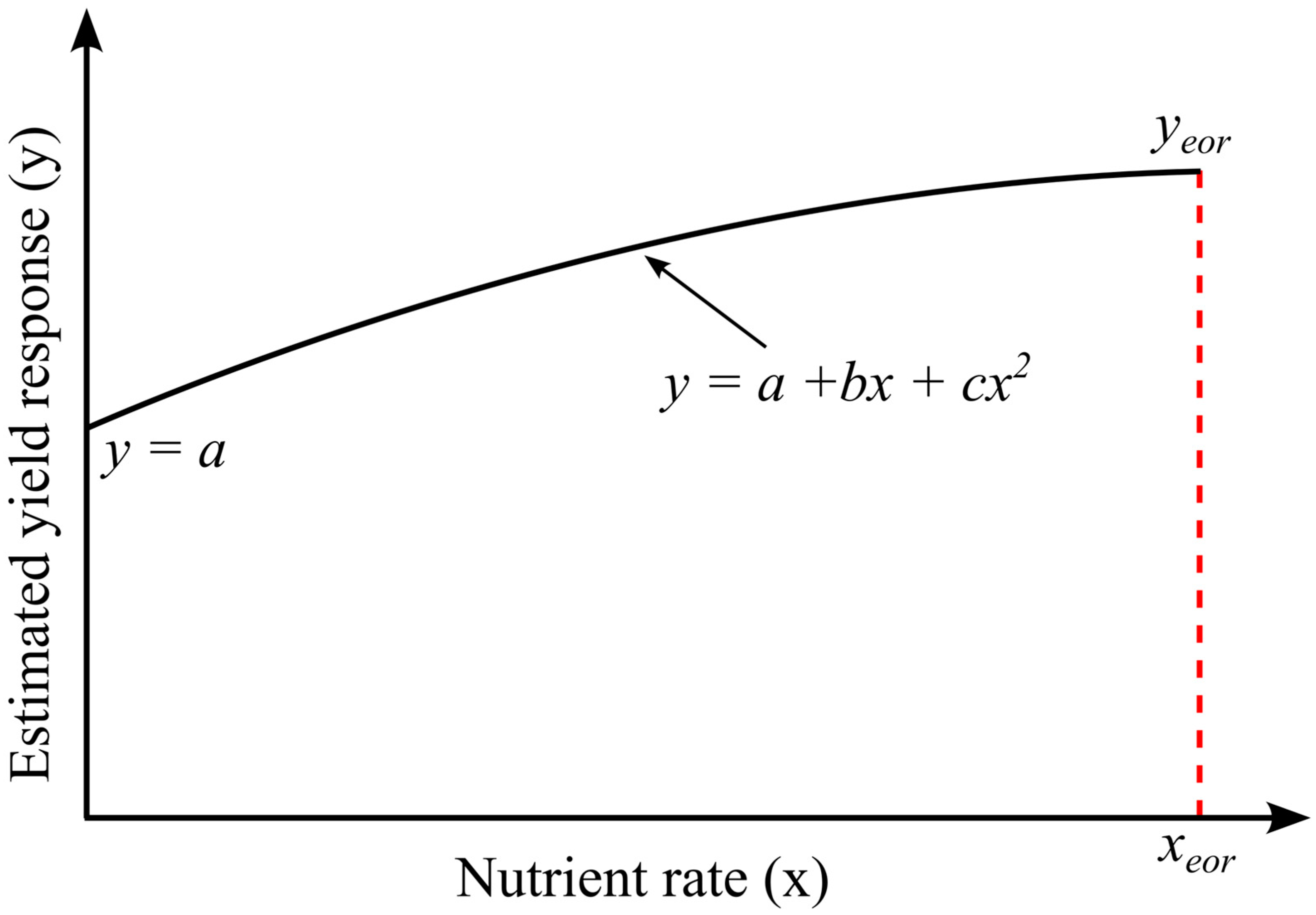
  71. Dhakal, C.; Lange, K. Crop yield response functions in nutrient application: A review. Agron. J. 2021, 113, 5222–5234. [Google Scholar] [CrossRef]
  72. Murrell, T.S. A Procedure for Estimating Yield Loss from Nutrient Rate Reductions; Report, International Plant Nutrition Institute: Norcross, GA, USA, 2009. [Google Scholar]
  73. Nasri, G.; Hajji, S.; Aydi, W.; Boughariou, E.; Allouche, N.; Bouri, S. Water vulnerability of coastal aquifers using AHP and parametric models: Methodological overview and a case study assessment. Arab. J. Geosci. 2021, 14, 59. [Google Scholar] [CrossRef]
  74. Nkeki, F.N.; Bello, E.I.; Agbaje, I.G. Flood risk mapping and urban infrastructural susceptibility assessment using a GIS and analytic hierarchical raster fusion approach in the Ona River Basin, Nigeria. Int. J. Disast. Risk Re. 2022, 77, 103097. [Google Scholar] [CrossRef]
  75. Yang, J.; Tang, Z.; Jiao, T.; Muhammad, A.M. Combining AHP and genetic algorithms approaches to modify DRASTIC model to assess groundwater vulnerability: A case study from Jianghan Plain, China. Environ. Earth Sci. 2017, 76, 426. [Google Scholar] [CrossRef]
  76. Barzegar, R.; Moghaddam, A.A.; Adamowski, J.; Nazemi, A.H. Delimitation of groundwater zones under contamination risk using a bagged ensemble of optimized DRASTIC frameworks. Environ. Sci. Pollut. Res. 2019, 26, 8325–8339. [Google Scholar] [CrossRef] [PubMed]
  77. Wu, H.; Chen, J.; Qian, H. A modified DRASTIC model for assessing contamination risk of groundwater in the northern suburb of Yinchuan, China. Environ. Earth Sci. 2016, 75, 483. [Google Scholar] [CrossRef]
Figure 1. Geographical location and boundaries of Nea Moudania basin (also showing the lowland and hilly areas delineated based on local hydrological conditions), along with the boundaries of the aquifer under study, the several administrative districts and settlements within the region and the water-supply wells (39 in total) used as critical receptors for observing nitrate concentrations.
Hydrology 11 00008 g001
Figure 2. Schematic representation of the methodological framework followed in the present study (E.C.—Export coefficients; RCH—Groundwater recharge; D.N.—Do-nothing scenario; F.R.S.—Fertilization reduction scenarios).
Hydrology 11 00008 g002
Figure 3. (a) Flow boundary conditions, along with the six distinct hydro-geological zones (HP zones) of the study area (defined based on a number of pumping tests in individual wells), and (b) the recharge zones in the study area (delineated based on several factors such as hydrological conditions, land use types and administrative boundaries).
Hydrology 11 00008 g003
Figure 4. (a) The abstraction wells (518 in total) operating in the region, and (b) hydraulic head distribution, along with groundwater flow direction in the Nea Moudania aquifer at the end of the calibration/validation period (2014).
Hydrology 11 00008 g004
Figure 5. (a) Boundary and initial conditions for the nitrate fate and transport model, and (b) distribution of annual nitrogen loading in the study area at a recharge zone level.
Hydrology 11 00008 g005
Figure 6. Percentages of on-ground nitrogen loadings from the different sources present in the study area.
Hydrology 11 00008 g006
Figure 7. Monthly on-ground nitrogen loading distribution for the study area.
Hydrology 11 00008 g007
Figure 8. A conceptual model of a quadratic response to a recommended nutrient rate [72].
Hydrology 11 00008 g008
Figure 9. Scatterplot of the simulated versus observed nitrate concentrations, along with the values of the several evaluation measures employed in the study and the locations of the observation wells (12 in total) used for nitrate concentration measurements.
Hydrology 11 00008 g009
Figure 10. Nitrate concentration (in mg/L) distribution under both the baseline (S0) and different fertilization reduction scenarios (S1–S5) by the end of the simulation period (2034).
Hydrology 11 00008 g010
Figure 11. Spatial distribution of nitrate concentration exceeding 25 mg/L under both the baseline (S0) and different fertilization reduction scenarios (S1–S5) by the end of the simulation period (2034).
Hydrology 11 00008 g011
Figure 12. Time-series of nitrate mass (in 106 kg) in the aquifer under study for both the baseline (S0) and different fertilization reduction scenarios (S1–S5) throughout the projection period (2014–2034).
Hydrology 11 00008 g012
Figure 13. Nitrate concentrations (in mg/L) in water-supply wells (critical receptors) under both the baseline (S0) and different fertilization reduction scenarios (S1–S5) by the end of the simulation period (2034).
Hydrology 11 00008 g013
Figure 14. Percentage income reduction for each crop under various fertilization reduction scenarios (S1–S5).
Hydrology 11 00008 g014
Table 1. The total population (including both permanent and seasonal residents), the corresponding number of wells used for water supply and the wastewater sources in each settlement [46,48].
SettlementsTotal PopulationWater-Supply WellsWastewater Sources
Nea Moudania25,04210Wastewater network
Nea Flogita45957Septic systems
Dionysiou13,1526Septic systems
Paralia DionysiouWastewater network
Portaria29835Septic systems
Zografou9032Septic systems
Ag. Panteleimon7623Septic systems
Simantra49316Septic systems
Table 2. Values of the various aquifer parameters as determined during the calibration/validation of the existing groundwater model (adapted from Siarkos and Latinopoulos, 2016 [49]).
ZoneHydraulic Conductivity (m/day)Effective Porosity/Specific YieldSpecific Storage (m−1)Longitudinal Dispersivity (m)Transverse Dispersivity (m)
10.5750.1500.00004757.5
20.5140.1250.00012
30.3250.1450.00019
40.1540.0700.00015
50.1140.0500.00006
60.3440.1400.00020
Table 3. Suggested amount of nitrogen per crop type (kg/ha) [57].
TreesGrainsVegetablesVineyards
OlivesApricotsOtherWheatOtherTomatoesOther
750150200150100350150150
Table 4. Nitrogen production per head for each animal type (kg/d) [59].
CattleSheepGoatsPigsPoultry
0.22500.01250.01350.05200.0011
Table 5. Export coefficients for the nitrogen sources present in the study area [50,54,61].
FertilizersIrrigation
Water
Wastewater
Sources
LivestockAtmospheric
Deposition
0.30–0.500.250.680.300.25
Table 6. Minimum, maximum and mean nitrate concentrations within the study area both at the beginning (2014) and end (2034) of the projection period under the various fertilizer application scenarios (S0–S5).
Metrics20142034
S0S1S2S3S4S5
Min1.20.10.10.10.10.10.1
Max31.854.651.949.246.544.043.0
Mean16.524.523.522.621.620.719.7
Table 7. Nitrate concentration (in mg/L) in the blended water provided by the corresponding water-supply wells to each settlement under the different fertilization reduction scenarios (S1–S5).
SettlementsS1S2S3S4S5
Nea Moudania26.625.724.823.923.0
Nea Flogita24.223.823.423.122.7
Dionysiou25.424.823.822.821.8
Paralia Dionysiou
Portaria25.624.523.522.421.3
Zografou41.439.537.535.533.6
Ag. Panteleimon13.613.112.612.111.5
Simantra20.320.019.619.319.0
Table 8. The agro-economic data related to the three crops analyzed in the present study and required for estimating crop-yield losses (all necessary data were acquired from the Directorate-General for Agricultural Economics and Veterinary of the Region of Central Macedonia, Greece).
Agro-Economic DataWheatOlivesApricots
Suggested rate of nitrogen (kg/ha)150750150
Cost of unit of nitrogen (EUR/kg)1.3751.3751.375
Price of unit of crop (EUR/kg)0.361.201.10
Expected yield (kg/ha)350015,00030,000
Expected yield with no nitrogen (kg/ha)1750750015,000
Table 9. Crop-yield losses (in kg/ha) for each crop and fertilization reduction scenario (S1–S5) (the percentage reduction in crop yield is given in parentheses).
ScenariosWheatOlivesApricots
S169 (2.0%)152 (1.0%)167 (0.6%)
S2162 (4.6%)438 (2.9%)630 (2.1%)
S3278 (7.9%)855 (5.7%)1389 (4.6%)
S4418 (11.9%)1406 (9.4%)2445 (8.2%)
S5581 (16.6%)2090 (13.9%)3797 (12.7%)
Table 10. Estimation of farmers’ annual income (EUR) for each type of crop considered in the economic analysis in the case of the baseline scenario (S0) (all necessary data were acquired from the Directorate-General for Agricultural Economics and Veterinary of the Region of Central Macedonia, Greece).
WheatOlivesApricots
a. Area (ha)4190.72502.0595.6
b. Crop yield (kg/ha)350015,00030,000
c. Total crop yield: (a*b) (kg)14,667,45037,530,00017,868,000
d. Selling price (EUR/kg)0.361.201.10
A. REVENUE: (c*d) (EUR)5,280,28245,036,00019,654,800
I. TOTAL REVENUE: (A) (EUR)5,280,28245,036,00019,654,800
e. Labor costs (EUR/ha)30013001600
f. Seed expenses (EUR/ha)1750.00.0
g. Nitrogen-rich fertilizers costs (EUR/ha)2061031206
h. Pesticides costs (EUR/ha)704801600
i. Materials expenses: (f+g+h) (EUR/ha)45115111806
B. TOTAL LABOR COSTS: (e*a) (EUR)1,257,2103,252,600952,960
C. TOTAL MATERIALS EXPENSES: (i*a) (EUR)1,891,0533,781,1481,075,803
D. OTHER COSTS: 5%*(A) (EUR)264,0142,251,800982,740
II. TOTAL COSTS: (B+C+D) (EUR)3,412,2779,285,5483,011,503
III. INCOME: (I–II) (EUR)1,868,00535,750,45316,643,298
Table 11. Estimated farmers’ annual income losses (EUR) for each crop, together with the total income losses resulting from the implementation of fertilization reduction scenarios (S1–S5).
ScenariosWheatOlivesApricotsTotal
S112,459381,94391,657486,059
S259,3151,146,091367,5451,572,951
S3139,1352,283,888827,6643,250,687
S4253,3533,803,8911,472,6365,529,880
S5400,5355,703,2462,301,8398,405,620
Table 12. Pair-wise comparison matrix for the predefined decision criteria (CR = 0.0 < 0.1), along with the results of criteria weights estimation.
CriteriaNitrate MassPopulationCostCPCRWeights
Nitrate mass1.0000.2500.7500.5000.12
Population4.0001.0003.0002.0000.48
Cost1.3330.3331.0000.6670.16
CPCR2.0000.5001.5001.0000.24
Table 13. The decision criteria’s values calculated for each fertilization reduction scenario (S1–S5), along with the corresponding scenario rankings (S3, which involves a 30% reduction in nitrogen-rich fertilizers was identified as the most suitable option for the area under study).
ScenariosNitrate (×106 kg)PopulationCost (EUR)CPCR (EUR/mg/L)Ranking
S149.542,080486,059567,5540.511
S247.425,9451,572,951995,8620.308
S345.59033,250,6871,379,5080.713
S443.69035,529,8801,763,4120.686
S541.79038,405,6202,152,4570.673
Disclaimer/Publisher’s Note: The statements, opinions and data contained in all publications are solely those of the individual author(s) and contributor(s) and not of MDPI and/or the editor(s). MDPI and/or the editor(s) disclaim responsibility for any injury to people or property resulting from any ideas, methods, instructions or products referred to in the content.

