Abstract
Estimating intensity−duration−frequency (IDF) curves requires local historical information of precipitation intensity. When such information is unavailable, as in areas without rain gauges, it is necessary to consider other methods to estimate curve parameters. In this study, three methods were explored to estimate IDF curves in ungauged areas: Kriging (KG), Inverse Distance Weighting (IDW), and Storm Index (SI). To test the viability of these methods, historical data collected from 31 rain gauges distributed in central Chile, 35° S to 38° S, are used. As a result of the reduced number of rain gauges to evaluate the performance of each method, we used LOOCV (Leaving One Out Cross Validation). The results indicate that KG was limited due to the sparse distribution of rain gauges in central Chile. SI (a linear scaling method) showed the smallest prediction error in all of the ungauged locations, and outperformed both KG and IDW. However, the SI method does not provide estimates of uncertainty, as is possible with KG. The simplicity of SI renders it a viable method for extrapolating IDF curves to locations without data in the central zone of Chile.
1. Introduction
Intensity−duration−frequency curves (IDF curves) are becoming increasingly important in the design of hydraulic works and in diverse areas of civil engineering [1,2,3,4,5]. IDF curves provide a statistical representation of historical rainfall intensity information for a given duration (Di) and return period (Ti) [6,7], although they go beyond mere data representation; they are also fundamental tools for flood risk reduction, playing a key role in the modeling and prediction of rainfall events [8]. By characterizing the statistical relationship between rainfall intensity, duration, and frequency, IDF curves enable engineers, urban planners, and decision makers to design and size infrastructure, such as stormwater drainage systems and flood barriers, to withstand extreme weather conditions [9]. In regions prone to intense flooding, the accurate estimation of IDF curves is critical for developing resilient infrastructure that can minimize property damage and protect human lives [10]. Thus, the significance of IDF curves extends from theoretical hydrological studies to tangible real-world applications that are central to sustainable urban development and disaster mitigation [11].
Several studies worldwide have focused on the development of IDF curves [12,13,14,15,16] for specific locations in Chile [17,18,19,20,21]. At the same time, other studies have focused on the estimation of IDF curves in areas with limited available information [5,22,23] and in the development of mathematical relationships between storm durations and return periods [7,24,25]. IDF curves are utilized in exploring climate change scenarios where extreme events seem to be becoming more frequent and intense [25,26,27]. A drawback of IDF curves is that they are valid for the area of influence of the station, so they cannot be directly extrapolated to other areas. Within this framework, various authors [22,28,29,30] have tried to regionalize IDF curves in order to estimate the precipitation intensity in ungauged areas.
Estimating IDF curves is not always straightforward, mostly due to the lack of data or the low spatio-temporal resolution of rainfall records. Access to rainfall intensity records of less than 1 h durations is also a big challenge [15,31,32]. As the lack of rain gauges is a common problem in Central Chile, this paper evaluates and compares the performance of three methods to interpolate/extrapolate IDF curves in mountainous locations of Central Chile.
IDF curves are constructed from stations with continuous precipitation records over time [33]. However, what happens for stations where rainfall amounts are only available for 24 h aggregation periods? In such cases, various methods have been suggested and applied in different parts of the world; for example, trend analysis and statistical downscaling [34]. However, the performance of each method depends on territorial singularities such as high variability of the topography, mountainous areas mixed with valley zones, and strong altitudinal gradients. For instance, Central Chile has a central valley delimited by the Andes Mountain range (peaks over 4000 m.a.s.l (meters above sea level)) to the east and a Coastal Mountain Range (peaks less than 400 m.a.s.l.) to the west, at the coast. Most of the rainfall comes from frontal systems from the Pacific Ocean and, in a smaller proportion, convective rains in the Andes Mountains. This situation marks an important rainfall variability, to which a latitudinal gradient is added, in which they increase from north to south and lack or have a poor coverage of rain gauges. Thus, it is necessary to compare different methods and establish which is the most appropriate for application in Chile, assuming an acceptable error, especially in mountainous areas such as most of Chile.
In addition to these challenges, climate change has significantly affected central Chile, where precipitation depth and intensity changes have been observed [35]. For instance, higher rainfall intensity and more runoff, leading to high water levels and flooding, have emphasized the need for reliable information, such as IDF curves, for the design, planning, and management of water infrastructure [36,37,38].
Hence, this study aims to assess the feasibility of using different estimation methods, including Kriging, Inverse Distance Weighted Method (IDW), and the Storm Index method proposed by Pizarro et al. [5], for constructing IDF curves at ungauged locations. The exploration of these methods responds to the urgent need to improve the estimation of IDF curves in data-sparse regions, thus contributing to effective flood protection infrastructure sizing.
2. Materials and Methods
The study area—central Chile—encompasses the Mataquito, Maule, and Biobío basins (Figure 1). The Mataquito and Maule basins have Mediterranean climates, with dry and wet seasons of equal duration. In contrast, the Biobío basin has a transition climate from a temperate Mediterranean to a humid Mediterranean [39]. Central Chile’s climate ranges from semi-arid to humid climates, and rainfall intensity varies in space due to the orographic effects of the Andes Mountain range [40]. From East to West is a valley region with elevations between 300 and 1000 m.a.s.l., and the Coastal Range has a longitudinal distance of less than 150 km.
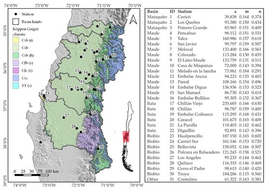
Figure 1.
Study area and location of the stations with IDF curves, where: a, m, and n are dimensionless parameters of the Bernard IDF equation. The Köppen–Geiger climatic classification is structured into three hierarchical orders across five types of climates, represented by the first capitalised letter, which follow latitudinal bands based on temperature and water availability. The second order, denoted by the following letter, pertains to precipitation. The third order is related to temperature. Additional letters in parentheses allow for further classification concerning mountain or ocean influence. More details on the climatic regionalisation of continental Chile can be found in Sarricolea et al. [41]. In the figure, the climates are as follows: Csb, Csb (i) Mediterranean (warm summer), Csb (h) Mediterranean (warm summer) with mountain influence, Csc Mediterranean (cool summer), Cfb (s) Marine West Coast (warm and dry summer), Cfc (s) Marine West Coast (cool and dry summer), and ET (s) Tundra with dry summer.
In general terms, the mean annual precipitation is 700 mm in the intermediate area between the Mataquito and Maule basins, but can exceed 2000 mm a year in the Andean mountains. In the Biobío basin, on the other hand, the mean annual precipitation is 1000 mm and can reach more than 3000 mm in the Andean mountains, which is largely made up of snow. This study considers stations (Figure 1) that are distributed between 18 and 1360 m.a.s.l. The number of years of available data, start year, and end year for all 31 stations are presented in Table S2 (see Supplementary Materials).
2.1. IDF Curves
The estimation of IDF curves demands the following variables: (1) rainfall intensity; (2) rainfall duration, which represents the temporal distribution of the storm; and (3) the number of years, in terms of probability for an event of a similar magnitude to occur [24,42]. Unesco. [19], as part of a 3-year research project, generated a set of 31 IDF curves, from paper pluviograms, after developing an optical curve reader. Tailor-made software enabled the automated construction of sub-daily IDF curves for durations from 15 min to 24 h, collecting and pre-serving large amounts of information easily, efficiently and with minimal error. Pluviograph band data from 31 stations are over two large territories: the area of influence of the Maule and the Biobío basin.
The Gumbel probability distribution function was used to obtain the return periods. This function is widely employed because of its capacity for modelling maximum intensities [43,44] and has been widely used for modelling precipitation data in Chile [18,19]. Rainfall intensities were estimated for durations of 1, 2, 4, 6, 12, and 24 h, for 5, 20, 50, and 100 years return periods. As obtaining the intensities from the IDF curve graphs is difficult, the data were fitted to the Bernard model (see Equation (1)), which has shown good results in Chile [19]. The Bernard model was one of the first models used for simultaneously estimating the empirical relationships between rainfall intensity, duration, and return period [18,45]. An advantage of this model is its direct and efficient computation [43]; therefore, it is among the most used models to represent these relationships [46]. The equation reads as follows:
where i represents rainfall intensity (mm/h) for a duration D (min) and a return period T (years), and a, m, and n are dimensionless parameters.
2.2. Spatial Interpolation and Extrapolation of IDF Curves
Methods for interpolating or extrapolating IDF curves at ungauged basins have been studied extensively [19]. However, selecting an appropriate method depends on the spatiotemporal resolution of the rainfall intensity records [47,48].
Ordinary Kriging. The application of geostatistical methods, such as Ordinary Kriging, are widely used across diverse scientific domains for spatial data interpolation [49,50]. Ordinary Kriging, in particular, provides a robust way to predict unknown values at unmeasured locations, offering a range of advantages over traditional interpolation methods. The general assumption of Ordinary Kriging is that there is an underlying constant mean process that is unknown. This contrasts with other forms of Kriging where the mean function is assumed to be a known (Simple Kriging), polynomial (Universal Kriging), or a regression function (Regression Kriging) [51].
Estimation using Kriging methods generally has two steps. First, it is necessary to determine the covariance structure of the data, typically through the estimation of a variogram. The empirical variogram is estimated by defining intervals (lags) and calculating the average semi-variance for all pairs of points within a specific lag distance. This process is repeated across 10–20 intervals to form the empirical variogram [52]. The variogram for lag distance h is defined as the average squared difference (or semi-variance) of values separated by h and is given by following:
where N(h) is the number of pairs for lag h, is the semi-variance, and z is the observed data at location u.
A suitable variogram model is then fitted to the empirical variogram, yielding the key parameters: sill (variance), range (distance over which spatial correlation exists), and nugget (micro-scale variation or measurement error). This first stage is pivotal to the accuracy of Kriging and might be sensitive to outliers or anomalous values [53].
The second step is the interpolation of data to generate predictions at locations with no data (Kriging). Ordinary Kriging [54] assumes a stochastic process, considering both the distance and the level of variation of observed data (a variogram) [55]. The unknown values are estimated based on a weighted sum of nearby observations, where proximity confers greater weight [56]. Equation (3) shows the sum of the weights, λi, multiplied by the observed data Zi, which estimates the prediction at a location. The value to predict comes from the weighted sum of the surrounding locations with measurements [57]. Setianto and Triandini [58] state that ordinary Kriging is unbiased if the sum of the weights is 1.
where is the estimated value at a certain point, λ denotes the weights, and Zi is a value of a known point.
The spatial structure of data must be evaluated to estimate the weights in the Kriging equations. The variogram can be estimated using a method of moments or maximum likelihood approach [59]. Kriging has various advantages over other methods. Firstly, it is a probabilistic model, and in addition to predicting a value, it also provides an estimate for the error or uncertainty [60]. The variogram enables the use of anisotropic covariances if the variation is directional. Modelling the variogram is crucial for accurate prediction; however, the variogram estimation process can break down in the presence of outliers and may require supervision.
The direct Kriging of distribution or function parameters for IDF curve estimation is not a new concept and has been explored in previous work [61,62,63]. Although it would be more appealing to model the random precipitation variable directly, data scarcity often necessitates a simpler, albeit less principled approach. Hence a less principled but appealing simpler approach is to evaluate its effectiveness compared to more established methods.
Ordinary Kriging is as a powerful spatial interpolation tool, aptly suited for complex tasks such as IDF curve estimation [64]. Its probabilistic nature, allowance for anisotropic covariances, and adaptability to different spatial structures make it the preferred method for many researchers and practitioners. However, careful handling of the variogram estimation and consideration of the method’s underlying assumptions are vital for obtaining reliable predictions. In the context of rainfall analysis and flood risk management, Kriging can offer valuable insights, provided that the data quality and methodological constraints are thoroughly addressed. For all analyses in this paper—Ordinary Kriging and IDW—the R software environment was used with the package gstat [65].
Inverse distance weighting. The inverse distance weighting technique (IDW) assumes closer points have greater weights than between points that are further apart, as stated in Equation (4).
where d is the distance between known points and the point to be estimated (see Equation (3) for more parameters).
Given that the computational complexity limits the efficient application of this method, a search radius is often used to select those points with data [66]. Although the value of the exponent can vary, the square of the distances is more frequent [58].
Comparing the performance of Kriging and IDW on interpolating parameters or intensities, Yao et al. [67] indicated that the network density affects the performance of these techniques. Almasi et al. [68] stated that when comparing Kriging with IDW, a better interpolator does not exist as the quality of the interpolation will depend on the spatial variation of the information. Liu et al. [50] suggested that Kriging is a better interpolator than IDW, but other studies indicate that IDW has similar or better results [67,69,70,71]. Much of the accuracy of the Kriging approach depends on the correct estimation of the variogram structure.
In Colombia, Becerra et al. [72] interpolated the parameters of the Gumbel distribution using IDW. The authors generated spatial maps for the parameters and the construction of IDF curves at an arbitrary location. The comparison with real intensities values showed errors of 10%.
Storm Index (k method). The storm index method, or k method, was developed by Pizarro et al. [5] and offers a practical approach for the construction of IDF curves for basins where continuous or high-resolution rainfall records are not available. Typically, this is achieved using pluviometer data from stations that have a hydrological behaviour similar to the station under study. The selection of a station that provides the k values (Ek) is crucial for the accuracy of the method. To select the station that provides the k values (Ek), Pizarro et al. [5] recommend stations where the differences between the intensities in 24 h are less than 2 mmh−1 as a selection criteria. This similarity in intensities ensures that the chosen station’s behaviour aligns well with the study area, allowing the derived k factors to be representative and accurate.
The core of the k-method consists of the generation of “k-factors”. These coefficients relate the intensity of rainfall for a specific duration to the intensity observed over a 24 h period. The expression for the k-factors is given by the following:
where Kij is the k factor for a duration i (hours) and return period j (years), Iij is the maximum intensity for the duration i and return period j, and I24j is the maximum intensity in 24 h for a return period j. The product between the k factors and the intensity in 24 h at the pluviometric station generates the intensity for the studied durations and hence enables the construction of the IDF curve.
The Storm Index method offers a practical approach for constructing IDF curves in areas where continuous or high-resolution rainfall records are not available. By relying on comparable stations and scaling the intensities with k factors, it bridges the data gap and provides valuable insights into the rainfall characteristics of ungauged or under-studied areas. However, the success of this method requires careful selection of the nearby station, considering the hydrological similarity and adherence to the specified intensity difference criteria. Moreover, while the method is relatively straightforward, it might require adjustments based on regional non-homogeneities or specific hydrological features of the study area.
The LOOCV methodology [73] allows for an evaluation of the above-listed methods. This process consists of leaving out one of the stations for predictions. The previously generated IDF curves within the study area that are known and fully validated in their parametric form, according to the Bernard equation (e.g., Unesco [19]), were used. For Kriging and IDW, the stations were systematically out, assuming that the parametric values of the Bernard equation are unknown for the station (a, m, and n). Next, the station’s parameters were estimated using each interpolation method to generate an estimation or infer its parametric behaviour for the IDF model for the station under study. The new IDF curve parameters were compared with the observed parameters for that particular station. In the case of the Storm Index, this method has a drawback. Thus, the LOOCV is a cross validation method that calculates the prediction error iteratively at the same time in a spatial location. Therefore, the prediction error is the average of the prediction errors for all iterations. This method captures the sensitivity of Kriging when few data are available. In the case of the Storm Index, LOOCV was not used.
In LOOCV, the possible number of comparisons would be n − 1, with n being the total number of stations. In this case, n = 31 stations, with their respective IDF curves [19]. However, as the intention was to compare the three IDF curve estimation methods for areas with missing data (Kriging, IDW, and Storm Index), the Storm Index restricted the rest of the methods because it can only be applied in those cases where the difference in 24 h rainfall intensities is less than 2 mm [5]. Nevertheless, it is always possible to apply it to each one of the stations because although one surrounding station does not fulfil the requirement, there would be another station that does fulfil it.
Goodness-of-Fit test. The goodness-of-fit compares intensity values for durations and return periods. As we have both observed intensity values and estimations carried out for each one of the methods for these same intensities, we were able to carry out statistical comparisons to determine the quality of such estimations. Thus, the Nash−Sutcliffe efficiency test (NSE) (Equation (6)), the Standard Error of Estimation (SEE) (Equation (7)), and the Mann−Whitney U test (U) (Equation (8)) were used:
where NSE is the Nash−Sutcliffe efficiency, SEE is the standard error of estimation (mm/h), U is the Mann−Whitney test, y is the observed values (mm/h), is the estimated values (mm/h), is the average of the observed values, n is the sample size, n1 is the size of the samples of the original data, n2 is the size of the samples of the estimated data, and R1 and R2 are rankings for samples R1 and R2, respectively.
NSE determines the relationship between the residual variance and the variance of the observed data [74,75]. Its values vary between −∞ and 1, where values closer to 1 indicate a better model fit [76]. In the case of the standard error of estimation [77,78], it shows the average deviation of the observed and modelled data; low SEE values indicate that the model fit is suitable and, according to Pizarro et al. [5], SEE values lower than 1.5 mmh−1 indicate an acceptable model fit. The Mann−Whitney U test is an alternative that is not parametric to Student’s t-test [79], which assumes that two samples come from the same distribution (H0) and can be used when small samples are available [80].
3. Results
Goodness-of-Fit of the Methods
The results for the combined durations and return periods for 31 stations for the NSE coefficient is shown in Figure 2 for the Kriging, IDW and Storm Index methods.
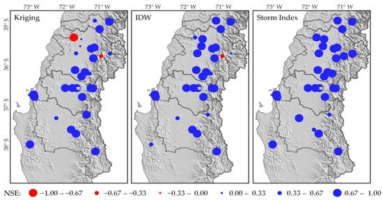
Figure 2.
Results of the goodness-of-fit test for the Nash-Sutcliffe coefficient (NSE) for the three methods under study: Kriging, Inverse Distance weighting (IDW), and Storm Index.
Table S1 (Supplementary Materials) shows the results for each station regarding the Nash−Sutcliffe efficiency coefficient, the standard error of estimation (mm/h), the result of the Mann−Whitney U test (p-value), and the station’s Ek are shown, as well as the Storm Index.
On average, NSE shows higher values for the Storm Index method than for Kriging and IDW (Table S1 in the Supplementary Materials). Similarly, in 26 out of 31 gauging stations, NSE exceeds a value of 0.9 for the Storm Index. In Kriging, it is higher in 12 of 31 and in IDW in 13 of 31. For NSE higher than 0.8, the Storm Index goes up to 28 of 31 comparisons, while the Kriging and IDW methods rise from 12 to 18 and 13 to 21, respectively. Regarding the standard estimation error, the Kriging and IDW methods exceed, on average, 3 mmh−1, whereas the Storm Index shows a lower value. If an error in the estimation of intensities of 2 mmh-1 is acceptable [5], Kriging (22 out of 31, 71%) and IDW (19 out of 31, 61%) exceeded this value, while the Storm Index achieved it in 9 of the 31 (29%) stations. Figure 3 shows the results for three stations for return periods of T = 5, 20, 50, and 100 years for all of the durations considered. The selected three stations shown were chosen as a representative sample of the data so that characteristics of the results could be highlighted. The results for the remaining 28 stations can be found in Supplementary Materials. The figures show that no method estimated the intensities well at lower durations (1 to 4 h), likely due to the high variability of precipitation at lower intensities. For durations longer than 5 h, Kriging and IDW overestimated the intensities. However, the Storm Index generally performed better.
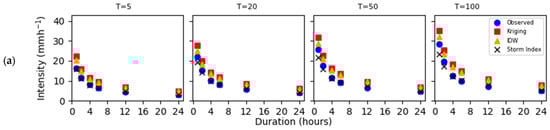
Figure 3.
IDF curves example for the Kriging, IDW, and Storm Index at stations (a) Curicó, (b) Talca, and (c) Troyo.
The Mann−Whitney U test results showed no significant difference between the observed and estimated intensities for the three methods considered (p > 0.05) in most of the stations. Only 4, 2, and 0 stations showed significant differences (p < 0.05) for Kriging, IDW, and the Storm Index, respectively. This situation could have been because of the dependence of this test on the size of the sample (24 samples) and the variation in the series of data [81] (Figure 4).
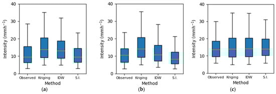
Figure 4.
Boxplot example for Kriging, IDW, and Storm Index for stations (a) Curicó (1), (b) Talca (5), and (c) Troyo (30).
4. Discussion
Various authors have found that the Kriging method obtains better results when interpolating data than IDW [57,82], while other authors have reported the opposite [83,84,85]. However, in this study, IDW was a better estimator of intensities than Kriging, possibly because of insufficient observations. The Kriging variogram fitting process can be particularly inefficient when sufficient data are unavailable [50].
Another important factor to address is the regionalization of IDF curves. Hershfield [86] designed precipitation intensity isolines for 30 min to 24 h and return periods of 1 to 100 years, limited to the continental United States. Similarly, Basumatari and Sil [87] constructed maps of rainfall intensities in the Barak River basin, India, for durations from 30 min to 24 h and return periods of 2 to 100 years. A similar approach was taken in Botswana, generating maps of 24 h intensities for return periods from 2 to 100 years [88]. This approach to regionalizing the IDF curves facilitates the creation of curves in areas without data. However, this approach limits estimates to the durations and return periods in the maps. On the other hand, various studies have preferred to regionalize the parameters of the equation to calculate IDF [30,44,86,87]. This approach has the advantage of allowing the IDF model in areas without data; therefore, IDF intensities are in a continuous spectrum. However, the results of the investigation by Rodríguez-Solà et al. [89], reported errors of up to 50% in the estimation of intensities of 1 h in the Iberian Peninsula, reducing to 20% for intensities greater than 2 h. Puricelli [90] used a similar strategy to regionalize the IDF curves of the Argentine Pampa, obtaining a good fit (r close to 0.9).
The results of this research, when regionalizing through spatial techniques (Kriging and IDW) were similar to Rodríguez-Solà et al. [89], that is, there was a significant error in the intensity estimates. However, when modelling using the storm index, the quality of the fit increased (Table S1 in the Supplementary Materials).
5. Conclusions
The results of this study demonstrate the high efficiency of the Storm Index method, compared with the Kriging and IDW methods, for estimating IDF curves in stations with missing data on mountainous areas of central Chile. The Kriging method generated the poorest results, as expected, as both methods require sufficiently spatially dense data [67], which was not the case in the study area, and underscore the drawback in areas with Mediterranean climates, mountainous terrains (i.e., high variability), and a low density of stations. One possibility would be to include expert opinions when determining the covariance structure rather than an empirical approach when few data are available, or an even more complex Bayesian approach that would allow for the principled integration of expert opinions with observed data.
The IDW method showed slightly better results than Kriging, seemingly because it does not require a variogram estimation, which can reduce prediction accuracy if the variogram model and its parameters are incorrectly specified or if precise estimation is problematic. However, the goodness-of-fit indices do not show large differences compared with the Kriging method.
The Storm Index method produced the best results. However, it is important to consider that this method has limitations for its application, as previously mentioned. Even so, considering these limitations, the Storm Index satisfactorily generates the best results for the territory under study for these cases.
Supplementary Materials
The following supporting information can be downloaded at: https://www.mdpi.com/article/10.3390/hydrology10090179/s1. Figure S1: Boxplots of intensities for the following stations; Figure S2: Boxplots of intensities for the following stations; Table S1: Summary of the goodness-of-fit tests; Table S2: Summary of data availability for each station in this study.
Author Contributions
Conceptualization, R.P., A.I. and C.S.; methodology, R.P., A.I., C.S. and F.B.; software, B.I.; validation, B.I. and A.I.; formal analysis, J.P.; investigation, P.G.-C. and D.R.; resources, F.P. (Felipe Pérez); data curation, F.P. (Felipe Pérez), F.B. and F.P. (Francisco Peña); writing—original draft preparation, A.I., B.I., J.P. and F.B.; writing—review and editing, B.I., C.S., F.P. (Francisco Peña), R.P., A.I., D.R. and P.G.-C. All authors have read and agreed to the published version of the manuscript.
Funding
This research received no external funding.
Data Availability Statement
Publicly available datasets were analyzed in this study. This data can be found here: http://www.cuhs.utalca.cl/ex-ctha/Docs/pdf/Publicaciones/libros/IDF_15_24_horas.pdf (accessed on 10 July 2023).
Acknowledgments
The authors thanks ANID BASAL FB210015. D.R. thanks the financial support from the Centro de Recursos Hídricos para la Agricultura y la Minería ANID/FONDAP/15130015.
Conflicts of Interest
The authors declare no conflict of interest.
References
- Link, G.A.; Watkins, D.W., Jr.; Johnson, D.L. Mapping Spatial Variation in Rainfall Intensity-Duration-Frequency Estimates Using a Geographical Information System. In Proceedings of the Joint Conference on Water Resource Engineering and Water Resources Planning and Management 2000, Minneapolis, MN, USA, 30 July–2 August 2000; pp. 1–10. [Google Scholar]
- Bara, M.; Gaál, L.; Szolgay, J.; Kohnová, S. Estimation of IDF Curves of Extreme Rainfall by Simple Scaling in Slovakia. Contributions to Geophysics and Geodesy. Contrib. Geophys. Geod. 2009, 39, 187–206. [Google Scholar]
- Asikoglu, O.L.; Benzeden, E. Simple Generalization Approach for Intensity-Duration-Frequency Relationships: Simple generalization approach for IDF relationships. Hydrol. Process. 2014, 28, 1114–1123. [Google Scholar] [CrossRef]
- Uboldi, F.; Sulis, A.N.; Lussana, C.; Cislaghi, M.; Russo, M. A Spatial Bootstrap Technique for Parameter Estimation of Rainfall Annual Maxima Distribution. Hydrol. Earth Syst. Sci. 2014, 18, 981–995. [Google Scholar] [CrossRef]
- Pizarro, R.; Valdés, R.; Abarza, A.; Garcia-Chevesich, P. A Simplified Storm Index Method to Extrapolate Intensity-Duration-Frequency (IDF) Curves for Ungauged Stations in Central Chile: Storm index method to extrapolate IDF curves. Hydrol. Process. 2015, 29, 641–652. [Google Scholar] [CrossRef]
- Langousis, A.; Veneziano, D. Intensity-Duration-Frequency Curves from Scaling Representations of Rainfall: Scaling representations of rainfall. Water Resour. Res. 2007, 43, W02422. [Google Scholar] [CrossRef]
- Elsebaie, I.H. Developing Rainfall Intensity–Duration–Frequency Relationship for Two Regions in Saudi Arabia. J. King Saud Univ.—Eng. Sci. 2012, 24, 131–140. [Google Scholar] [CrossRef]
- Sivapalan, M.; Blöschl, G. Time Scale Interactions and the Coevolution of Humans and Water: Time scale interactions and coevolution of humans and water. Water Resour. Res. 2015, 51, 6988–7022. [Google Scholar] [CrossRef]
- Chow, V.T.; Maidment, D.; Mays, L. Hidrología Aplicada; McGraw-Hill: Bogotá, Colombia, 2000; ISBN 978-958-600-171-7. [Google Scholar]
- Simonović, S.P. Floods in a Changing Climate. Risk Management; International Hydrology Series; Cambridge University Press: Cambridge, UK, 2012; ISBN 978-1-107-01874-7. [Google Scholar]
- Kundzewicz, Z.W.; Kanae, S.; Seneviratne, S.I.; Handmer, J.; Nicholls, N.; Peduzzi, P.; Mechler, R.; Bouwer, L.M.; Arnell, N.; Mach, K.; et al. Flood Risk and Climate Change: Global and Regional Perspectives. Hydrol. Sci. J. 2014, 59, 1–28. [Google Scholar] [CrossRef]
- Singh, V.P.; Zhang, L. IDF Curves Using the Frank Archimedean Copula. J. Hydrol. Eng. 2007, 12, 651–662. [Google Scholar] [CrossRef]
- Burn, D.H. A Framework for Regional Estimation of Intensity-Duration-Frequency (IDF) Curves: Regional estimation of intensity-duration-frequency (IDF) curves. Hydrol. Process. 2014, 28, 4209–4218. [Google Scholar] [CrossRef]
- Mirhosseini, G.; Srivastava, P.; Sharifi, A. Developing Probability-Based IDF Curves Using Kernel Density Estimator. J. Hydrol. Eng. 2015, 20, 04015002. [Google Scholar] [CrossRef]
- Sušin, N.; Peer, P. Open-Source Tool for Interactive Digitisation of Pluviograph Strip Charts. Weather 2018, 73, 222–226. [Google Scholar] [CrossRef]
- Casas-Castillo, M.C.; Rodríguez-Solà, R.; Navarro, X.; Russo, B.; Lastra, A.; González, P.; Redaño, A. On the Consideration of Scaling Properties of Extreme Rainfall in Madrid (Spain) for Developing a Generalized Intensity-Duration-Frequency Equation and Assessing Probable Maximum Precipitation Estimates. Theor. Appl. Climatol. 2018, 131, 573–580. [Google Scholar] [CrossRef]
- Espíldora, B. Estimación de Curvas Intensidad-Duración-Frecuencia Mediante Coeficientes Generalizados. In Proceedings of the I Coloquio Nacional Sociedad Chilena de Ingeniería, Sociedad Chilena de Ingeniería Hidráulica, Santiago, Chile, 30 June–2 July 1971. [Google Scholar]
- UNESCO. Curvas Intensidad–Duración–Frecuencia para la Zona Centro sur de Chile; Documento Técnico del PHI-LAC; PHI-LAC: Montevideo, Uruguay, 2007; ISBN 978-92-9089-100-0. [Google Scholar]
- UNESCO. Curvas Intensidad Duración Frecuencia para las Regiones Metropolitana, Maule y Biobío. Intensidades Desde 15 Minutos a 24 Horas; Documento Técnico del PHI-LAC; PHI-LAC: Montevideo, Uruguay, 2013; ISBN 978-92-9089-189-5. [Google Scholar]
- Soto, X.; Meier, C. Subestimación de Los Valores IDF En Concepción. 1: Derivación Completa y Comparación Con Otras Metodologías. In Proceedings of the XXI Congreso Chileno de Hidráulica, Concepción, Chile, 23–25 October 2013. [Google Scholar]
- Soto, C. Construcción de Curvas Intensidad-Duración-Frecuencia, de Alta Resolución Espacial Para La Zona Centro-Sur de Chile; Universidad de la Frontera: Temuco, Chile, 2019. [Google Scholar]
- Alila, Y. A Hierarchical Approach for the Regionalization of Precipitation Annual Maxima in Canada. J. Geophys. Res. Atmos. 1999, 104, 31645–31655. [Google Scholar] [CrossRef]
- Liew, S.; Raghavan, S.V.; Liong, S.-Y. Development of Intensity-Duration-Frequency Curves at Ungauged Sites: Risk Management under Changing Climate. Geosci. Lett. 2014, 1, 8. [Google Scholar] [CrossRef][Green Version]
- Mauriño, M.F. Generalized Rainfall-Duration-Frequency Relationships: Applicability in Different Climatic Regions of Argentina. J. Hydrol. Eng. 2004, 9, 269–274. [Google Scholar] [CrossRef]
- Mailhot, A.; Duchesne, S.; Caya, D.; Talbot, G. Assessment of Future Change in Intensity–Duration–Frequency (IDF) Curves for Southern Quebec Using the Canadian Regional Climate Model (CRCM). J. Hydrol. 2007, 347, 197–210. [Google Scholar] [CrossRef]
- Zhu, J.; Stone, M.C.; Forsee, W. Analysis of Potential Impacts of Climate Change on Intensity–Duration–Frequency (IDF) Relationships for Six Regions in the United States. J. Water Clim. Change 2012, 3, 185–196. [Google Scholar] [CrossRef]
- Liew, S.C.; Raghavan, S.V.; Liong, S.-Y. How to Construct Future IDF Curves, under Changing Climate, for Sites with Scarce Rainfall Records?: Derivation of IDF curves for ungauged sites. Hydrol. Process. 2014, 28, 3276–3287. [Google Scholar] [CrossRef]
- Madsen, H.; Mikkelsen, P.S.; Rosbjerg, D.; Harremoës, P. Regional Estimation of Rainfall Intensity-Duration-Frequency Curves Using Generalized Least Squares Regression of Partial Duration Series Statistics: Regional estimation of rainfall IDF curves. Water Resour. Res. 2002, 38, 21-1–21-11. [Google Scholar] [CrossRef]
- Salas, L.; Fernández, J. Nueva Metodología Para El Análisis de La Variable Intensidad Máxima Anual de Precipitación. Ecología 2006, 20, 435–440. [Google Scholar]
- Soltani, S.; Helfi, R.; Almasi, P.; Modarres, R. Regionalization of Rainfall Intensity-Duration-Frequency Using a Simple Scaling Model. Water Resour. Manag. 2017, 31, 4253–4273. [Google Scholar] [CrossRef]
- Svensson, C.; Clarke, R.T.; Jones, D.A. An Experimental Comparison of Methods for Estimating Rainfall Intensity-Duration-Frequency Relations from Fragmentary Records. J. Hydrol. 2007, 341, 79–89. [Google Scholar] [CrossRef]
- Jaklič, A.; Šajn, L.; Derganc, G.; Peer, P. Automatic Digitization of Pluviograph Strip Charts: Automatic Digitization of Pluviograph Strip Charts. Meteorol. Appl. 2016, 23, 57–64. [Google Scholar] [CrossRef]
- Yu, P.-S.; Chen, C.-J. Potential of extending the rainfall intensity–duration–frequency relationship to non-recording rain gauges. Hydrol. Process. 1997, 11, 377–390. [Google Scholar] [CrossRef]
- Willems, P.; Arnbjerg-Nielsen, K.; Olsson, J.; Nguyen, V.T.V. Climate Change Impact Assessment on Urban Rainfall Extremes and Urban Drainage: Methods and Shortcomings. Atmos. Res. 2012, 103, 106–118. [Google Scholar] [CrossRef]
- Jacques-Coper, M.; Garreaud, R.D. Characterization of the 1970s Climate Shift in South America: Characterization of the 1970 S climate shift in south America. Int. J. Climatol. 2015, 35, 2164–2179. [Google Scholar] [CrossRef]
- Jordan, T.; Riquelme, R.; González, G.; Herrera, C.; Godfrey, L.; Colucci, S.; Gironás, J.; Gamboa, C.; Urrutia, J.; Tapia, L.; et al. Hydrological and Geomorphological Consequences of the Extreme Precipitation Event of 24–26 March 2015, Chile. In Proceedings of the Los Aluviones de Atacama, Contexto, Causas y Efectos, La Serena, Chile, 1 October 2015; pp. 777–780. [Google Scholar]
- Pizarro, R.; Ingram, B.; Gonzalez-Leiva, F.; Valdés-Pineda, R.; Sangüesa, C.; Delgado, N.; García-Chevesich, P.; Valdés, J. WEBSEIDF: A Web-Based System for the Estimation of IDF Curves in Central Chile. Hydrology 2018, 5, 40. [Google Scholar] [CrossRef]
- Pizarro-Tapia, R.; González-Leiva, F.; Valdés-Pineda, R.; Ingram, B.; Sangüesa, C.; Vallejos, C. A Rainfall Intensity Data Rescue Initiative for Central Chile Utilizing a Pluviograph Strip Charts Reader (PSCR). Water 2020, 12, 1887. [Google Scholar] [CrossRef]
- Pizarro, R.; Valdés, R.; García-Chevesich, P.; Vallejos, C.; Sangüesa, C.; Morales, C.; Balocchi, F.; Abarza, A.; Fuentes, R. Latitudinal Analysis of Rainfall Intensity and Mean Annual Precipitation in Chile [Análisis Latitudinal de La Intensidad de Lluvias y Precipitación Media Anual En Chile]. Chil. J. Agric. Res. 2012, 72, 252–261. [Google Scholar] [CrossRef]
- Kono, M.; Fukao, Y.; Yamamoto, A. Mountain Building in the Central Andes. J. Geophys. Res. Solid Earth 1989, 94, 3891–3905. [Google Scholar] [CrossRef]
- Sarricolea, P.; Herrera-Ossandon, M.; Meseguer-Ruiz, Ó. Climatic Regionalisation of Continental Chile. J. Maps 2017, 13, 66–73. [Google Scholar] [CrossRef]
- Willems, P. Compound Intensity/Duration/Frequency-Relationships of Extreme Precipitation for Two Seasons and Two Storm Types. J. Hydrol. 2000, 233, 189–205. [Google Scholar] [CrossRef]
- Koutsoyiannis, D.; Kozonis, D.; Manetas, A. A Mathematical Framework for Studying Rainfall Intensity-Duration-Frequency Relationships. J. Hydrol. 1998, 206, 118–135. [Google Scholar] [CrossRef]
- Wayal, A.; Menon, K. Intensity-Duration-Frequency Curves and Regionalisation. International. International. J. Innov. Res. Adv. Eng. 2014, 1, 28–32. [Google Scholar]
- Pereyra-Díaz, D.; Pérez-Sesma, J.; Gómez-Romero, L. Ecuaciones Que Estiman Las Curvas Intensidad-Duración- Periodo de Retorno de La Lluvia. GEOS 2004, 24, 46–56. [Google Scholar]
- Gutiérrez-López, A.; Barragán-Regalado, R. Ajuste de Curvas IDF a Partir de Tormentas de Corta Duración. Tecnol. Cienc. Agua 2019, 10, 01–24. [Google Scholar] [CrossRef]
- Chandra, R.; Saha, U.; Mujumdar, P.P. Model and Parameter Uncertainty in IDF Relationships under Climate Change. Adv. Water Resour. 2015, 79, 127–139. [Google Scholar] [CrossRef]
- Paixao, E.; Mirza, M.M.Q.; Shephard, M.W.; Auld, H.; Klaassen, J.; Smith, G. An Integrated Approach for Identifying Homogeneous Regions of Extreme Rainfall Events and Estimating IDF Curves in Southern Ontario, Canada: Incorporating Radar Observations. J. Hydrol. 2015, 528, 734–750. [Google Scholar] [CrossRef]
- Cao, R.; Zee Ma, Y.; Gomez, E. Geostatistical Applications in Petroleum Reservoir Modelling. J. South. Afr. Inst. Min. Metall. 2014, 114, 625–631. [Google Scholar]
- Liu, W.; Du, P.; Zhao, Z.; Zhang, L. An Adaptive Weighting Algorithm for Interpolating the Soil Potassium Content. Sci. Rep. 2016, 6, 23889. [Google Scholar] [CrossRef] [PubMed]
- Goovaerts, P. Geostatistics for Natural Resources Evaluation; Applied Geostatistics Series; Oxford University Press: New York, NY, USA, 1997; ISBN 978-0-19-511538-3. [Google Scholar]
- Cressie, N.A.C. Statistics for Spatial Data; John Wiley & Sons, Inc.: New York, NY, USA, 1993. [Google Scholar]
- Chiles, J.-P.; Delfiner, P. Geostatistics: Modeling Spatial Uncertainty, 2nd ed.; Wiley Series in Probability and Statistics; Wiley: Hoboken, NJ, USA, 2012; ISBN 978-0-470-18315-1. [Google Scholar]
- Yang, X.; Xie, X.; Liu, D.L.; Ji, F.; Wang, L. Spatial Interpolation of Daily Rainfall Data for Local Climate Impact Assessment over Greater Sydney Region. Adv. Meteorol. 2015, 2015, 563629. [Google Scholar] [CrossRef]
- Chaplot, V.; Darboux, F.; Bourennane, H.; Leguédois, S.; Silvera, N.; Phachomphon, K. Accuracy of Interpolation Techniques for the Derivation of Digital Elevation Models in Relation to Landform Types and Data Density. Geomorphology 2006, 77, 126–141. [Google Scholar] [CrossRef]
- Azpurua, M.A.; Ramos, K.D. A Comparison of Spatial Interpolation Methods for Estimation of Average Electromagnetic Field Magnitude. Prog. Electromagn. Res. M 2010, 14, 135–145. [Google Scholar] [CrossRef]
- Yasrebi, J.; Fathi, H.; Karimian, N.; Moazallahi, M.; Gazni, R. Evaluation and Comparison of Ordinary Kriging and Inverse Distance Weighting Methods for Prediction of Spatial Variability of Some Soil Chemical Parameters. Res. J. Biol. Sci. 2009, 4, 93–102. [Google Scholar]
- Setianto, A.; Triandini, T. Comparison of Kriging and Inverse Distance Weighted (IDW) Interpolation Methods in Lineament Extraction and Analysis. J. Appl. Geol. 2013, 5. [Google Scholar] [CrossRef]
- Lark, R.M. Estimating Variograms of Soil Properties by the Method-of-Moments and Maximum Likelihood: Estimating Variograms. Eur. J. Soil Sci. 2000, 51, 717–728. [Google Scholar] [CrossRef]
- Lobato-Sanchez, R.; Aparicio-Mijares, F.; Sosa-Chinas, M.; Mendoza-Uribe, I. Caracterización Espacial de Redes Pluviográficas: Caso de La Cuenca de La Presa Peñitas. Tecnol. Cienc. Agua 2012, 3, 103–121. [Google Scholar]
- Moncho, R.; Belda, F.; Caselles, V. Climatic Study of the Exponent “n” in IDF Curves: Application for the Iberian Peninsula. Tethys J. Weather Clim. West. Mediterr. 2009, 6, 3–14. [Google Scholar] [CrossRef]
- Szolgay, J.; Parajka, J.; Kohnová, S.; Hlavčová, K. Comparison of Mapping Approaches of Design Annual Maximum Daily Precipitation. Atmos. Res. 2009, 92, 289–307. [Google Scholar] [CrossRef]
- Shehu, B.; Willems, W.; Stockel, H.; Thiele, L.; Haberlandt, U. Regionalisation of Rainfall Depth-Duration-Frequency Curves in Germany. Hydrometeorol./Model. Approaches 2022. [Google Scholar] [CrossRef]
- Teegavarapu, R.S.V. Floods in a Changing Climate: Hydrologic Modeling; Cambridge University Press: Cambridge, UK, 2012. [Google Scholar]
- Pebesma, E.J. Multivariable Geostatistics in S: The Gstat Package. Comput. Geosci. 2004, 30, 683–691. [Google Scholar] [CrossRef]
- Papari, G.; Petkov, N. Reduced Inverse Distance Weighting Interpolation for Painterly Rendering. In Computer Analysis of Images and Patterns; Jiang, X., Petkov, N., Eds.; Lecture Notes in Computer Science; Springer Berlin Heidelberg: Berlin/Heidelberg, Germany, 2009; Volume 5702, pp. 509–516. ISBN 978-3-642-03766-5. [Google Scholar]
- Yao, X.; Fu, B.; Lü, Y.; Sun, F.; Wang, S.; Liu, M. Comparison of Four Spatial Interpolation Methods for Estimating Soil Moisture in a Complex Terrain Catchment. PLoS ONE 2013, 8, e54660. [Google Scholar] [CrossRef] [PubMed]
- Almasi, A.; Jalalian, A.; Toomanian, N. Using OK and IDW Methods for Prediction the Spatial Variability of A Horizon Depth and OM in Soils of Shahrekord, Iran. J. Environ. Earth Sci. 2014, 4, 17–27. [Google Scholar]
- Dodson, R.; Marks, D. Daily Air Temperature Interpolated at High Spatial Resolution over a Large Mountainous Region. Clim. Res. 1997, 8, 1–20. [Google Scholar] [CrossRef]
- Villatoro, M.; Henríquez, C.; Sancho, F. Comparación de Los Interpoladores IDW y Kriging En La Variación Espacial de Ph, ca, Cice y p Del Suelo. Agron. Costarric. 2008, 32, 95–105. [Google Scholar]
- Gong, G.; Mattevada, S.; O’Bryant, S.E. Comparison of the Accuracy of Kriging and IDW Interpolations in Estimating Groundwater Arsenic Concentrations in Texas. Environ. Res. 2014, 130, 59–69. [Google Scholar] [CrossRef]
- Becerra Oviedo, J.A.; Sánchez Mazorca, L.F.; Acosta Castellano, P.M.; Díaz Arévalo, J.L. Regionalización de Curvas IDF Para El Uso de Modelos Hidrometeorológicos En La Sabana Occidental Del Departamento de Cundinamarca. Ing. Región 2015, 14, 143. [Google Scholar] [CrossRef]
- Kumari, M.; Basistha, A.; Bakimchandra, O.; Singh, C.K. Comparison of Spatial Interpolation Methods for Mapping Rainfall in Indian Himalayas of Uttarakhand Region. In Geostatistical and Geospatial Approaches for the Characterization of Natural Resources in the Environment; Raju, N.J., Ed.; Springer International Publishing: Cham, Switzerland, 2016; pp. 159–168. ISBN 978-3-319-18662-7. [Google Scholar]
- Nash, J.E.; Sutcliffe, J.V. River Flow Forecasting through Conceptual Models Part I—A Discussion of Principles. J. Hydrol. 1970, 10, 282–290. [Google Scholar] [CrossRef]
- Esquivel, G.; Sánchez, I.; Velásquez, M.; López, A.; López, R.; Bueno, P. Modelación Del Escurrimiento En Una Subcuenca Del Trópico Húmedo de México y Su Análisis Mediante Indices de Eficiencia Predictiva. Agrofaz 2013, 13, 113–118. [Google Scholar]
- Moriasi, D.N.; Arnold, J.G.; van Liew, M.W.; Bingner, R.L.; Harmel, R.D.; Veith, T.L. Veith Model Evaluation Guidelines for Systematic Quantification of Accuracy in Watershed Simulations. Trans. ASABE 2007, 50, 885–900. [Google Scholar] [CrossRef]
- Beard, L. Statistical Methods in Hydrology; U.S. Army Engineer District Corps of Engineers: Sacramento, CA, USA, 1962. [Google Scholar]
- Torres, V.; Barbosa, I.; Meyer, R.; Noda, A.; Sarduy, L. Criterios de Bondad de Ajuste En La Selección de Modelos No Lineales En La Descripción de Comportamientos Biológicos. Rev. Cuba. Cienc. Agrícola 2012, 46, 345–350. [Google Scholar]
- Fagerland, M.W. T-Tests, Non-Parametric Tests, and Large Studies—A Paradox of Statistical Practice? BMC Med. Res. Methodol. 2012, 12, 78. [Google Scholar] [CrossRef]
- Nachar, N. The Mann-Whitney U: A Test for Assessing Whether Two Independent Samples Come from the Same Distribution. Tutor. Quant. Methods Psychol. 2008, 4, 13–20. [Google Scholar] [CrossRef]
- Yue, S.; Pilon, P.; Cavadias, G. Power of the Mann–Kendall and Spearman’s Rho Tests for Detecting Monotonic Trends in Hydrological Series. J. Hydrol. 2002, 259, 254–271. [Google Scholar] [CrossRef]
- Liu, G.; Yang, X. Spatial Variability Analysis of Soil Properties within a Field. In Computer and Computing Technologies in Agriculture, Volume II; Li, D., Ed.; The International Federation for Information Processing; Springer: Boston, MA, USA, 2008; Volume 259, pp. 1341–1344. ISBN 978-0-387-77252-3. [Google Scholar]
- Weber, D.; Englund, E. Evaluation and Comparison of Spatial Interpolators. Math. Geol. 1992, 24, 381–391. [Google Scholar] [CrossRef]
- Gotway, C.A.; Ferguson, R.B.; Hergert, G.W.; Peterson, T.A. Comparison of Kriging and Inverse-Distance Methods for Mapping Soil Parameters. Soil Sci. Soc. Am. J. 1996, 60, 1237–1247. [Google Scholar] [CrossRef]
- Li, J.; Heap, A.D. A Review of Comparative Studies of Spatial Interpolation Methods in Environmental Sciences: Performance and Impact Factors. Ecol. Inform. 2011, 6, 228–241. [Google Scholar] [CrossRef]
- Hershfield, D. Rainfall Frequency Atlas of the United States for Durations from 30 Minutes to 24 Hour and Return Periods from 1 to 100 Years; Technical Paper; Department of Commerce: Washington, DC, USA, 1961. [Google Scholar]
- Basumatary, V.; Sil, B. Generation of Rainfall Intensity-Duration-Frequency Curves for the Barak River Basin. Meteorol. Hydrol. Water Manag. 2017, 6, 47–57. [Google Scholar] [CrossRef]
- Alemaw, B.F.; Chaoka, R.T. Regionalization of Rainfall Intensity-Duration-Frequency (IDF) Curves in Botswana. J. Water Resour. Prot. 2016, 8, 1128–1144. [Google Scholar] [CrossRef][Green Version]
- Rodríguez-Solà, R.; Casas-Castillo, M.C.; Navarro, X.; Redaño, Á. A Study of the Scaling Properties of Rainfall in Spain and Its Appropriateness to Generate Intensity-Duration-Frequency Curves from Daily Records: A study of scaling rainfall properties in Spain to generate IDF curves. Int. J. Climatol. 2017, 37, 770–780. [Google Scholar] [CrossRef]
- Puricelli, M. Rainfall Extremes Modeling under Shortage of Data and Uncertainty in the Pampean Region (Argentina). Cuad. Investig. Geográfica 2018, 44, 719. [Google Scholar] [CrossRef]
Disclaimer/Publisher’s Note: The statements, opinions and data contained in all publications are solely those of the individual author(s) and contributor(s) and not of MDPI and/or the editor(s). MDPI and/or the editor(s) disclaim responsibility for any injury to people or property resulting from any ideas, methods, instructions or products referred to in the content. |
© 2023 by the authors. Licensee MDPI, Basel, Switzerland. This article is an open access article distributed under the terms and conditions of the Creative Commons Attribution (CC BY) license (https://creativecommons.org/licenses/by/4.0/).