Article

Predictive MPC-Based Operation of Urban Drainage Systems Using Input Data-Clustered Artificial Neural Networks Rainfall Forecasting Models

by
Fatemeh Jafari
1,
S. Jamshid Mousavi
2,* and
Kumaraswamy Ponnambalam
3,*
1
Faculty of Electrical and Computer Engineering, University of Waterloo, Waterloo, ON N2L 5R5, Canada
2
Faculty of Civil and Environmental Engineering, Amirkabir University of Technology (Tehran Polytechnic), Tehran 15875-4413, Iran
3
Department of Systems Design Engineering, University of Waterloo, Waterloo, ON N2L 5R5, Canada
*
Authors to whom correspondence should be addressed.
Hydrology 2023, 10(7), 139; https://doi.org/10.3390/hydrology10070139
Submission received: 18 May 2023 / Revised: 15 June 2023 / Accepted: 26 June 2023 / Published: 29 June 2023

Abstract

:
The model predictive control (MPC) approach can be implemented in either a reactive (RE-) or predictive (PR-) manner to control the operation of urban drainage systems (UDSs). Previous research focused mostly on the RE-MPC, as the PR-MPC, despite its potential to improve the performance of the UDS operations, requires additional computational resources and is more complex. This research evaluates the conditions under which the PR-MPC approach may be preferable. A PR-MPC model is developed, consisting of an adaptive input data-clustered ANN-based rainfall forecasting method coupled to an MPC framework. Observed and forecasted rainfall events are inputs to the internal MPC model, including the rainfall-runoff SWMM simulation model of the system and the MPC optimizer, which is a harmony search-based model determining optimal control policies. The proposed model was used as part of the UDS of Tehran, Iran, under different scenarios of input (rainfall), forecast accuracy (IFAC), and time horizon (IFTH). Results indicate that the PR-MPC performs better for longer-duration rainfall events, while the RE-MPC could be used to control very short storm occurrences. The proposed PR-MPC model can achieve between 85 and 92% of the performance of an ideal model functioning under the premise of perfect, error-free rainfall forecasts for two investigated rainfall events. Additionally, the IFAC can be improved by including rainfall fluctuations over finer temporal resolutions than the forecast horizon as additional predictors.

1. Introduction

Extreme rainfall-caused urban flooding is one of the most destructive natural catastrophes in the world [1], but with effective management, it can become a valuable human resource [2]. Climate change and modifications in human settlement patterns are the two primary causes of urban pluvial floods as a result of global change [3]. Adding new pipelines, storage facilities, and channels or increasing the capacity of existing infrastructure pieces is a fundamental answer [4,5]. This decreases the risk of flooding by accelerating the transport of water; however, such a solution may be costly and not always a viable option due to the lengthy implementation period and lack of land [6]. Urban drainage systems (UDSs) that convey stormwater away from cities can also be managed with nonstructural measures, such as optimizing operation policies with intelligent control approaches [6,7,8,9,10,11]. Computationally effective stochastic optimization models have been successfully implemented in optimizing reservoir system operations, e.g., [12,13], which are yet to be applied in UDSs. In this area of work, pre-emptive prediction of floods using enhanced rainfall forecasting algorithms can afford us additional possibilities to optimally employ flood control devices. Online and real-time control (RTC) systems have been widely used in flash flood warning applications [14] that utilize short-term rainfall predictions. Implementing intelligent RTC techniques makes UDS management “smart” by transforming passive operational units into active adaptive units that can respond more flexibly to oncoming floods [15]. Model predictive control (MPC) is an adaptive control approach for applying advanced RTC in which the optimal control rules are recursively modified based on newly obtained information about the system’s state and present and predicted rainfall loads. This strategy can be implemented either reactively or predictively in terms of input time [6,8]. In the former method, the system responds to current and possibly historical data, whereas the latter refers to the management of the system based on current information and the estimation of future random inputs to the system [6,8]. Several recent studies utilized the reactive RTC technique, as well as reactive MPC (Re-MPC), to establish optimal rules for the regulation of the controllable elements of the UDS, such as pumps and gates [7,16,17,18,19,20,21,22,23,24,25,26,27,28,29,30]. The predictive RTC technique has also been investigated [31,32,33,34], albeit with significantly fewer applications. This is due to the additional computational resources required for adaptively implementing a predictive RTC model, especially the predictive MPC (PR-MPC) approach, and uncertainties associated with rainfall forecasting, so the optimal solutions found will be under the influence of forecast errors. Consequently, it is crucial and necessary to verify the efficacy and precision of rainfall forecasting approaches, particularly for short-term prediction, prior to implementing them in the RTC of UDS.
Rainfall is a complex and highly nonlinear hydrologic process in nature that depends on a number of temporal and spatial variables [35]; therefore, despite the advancements in technology and models, it still entails a high degree of uncertainty and the possibility of prediction error [36]. In tiny, urbanized areas, rainfall forecasts at short intervals of 5 to 30 min would be more essential [37], as their small size and large proportion of impervious surfaces result in a rapid hydrologic response [38]. Luk et al. conducted a sensitivity study to determine the optimal input data combination for training an artificial neural network (ANN)-based precipitation prediction model for the next 15 min [38]. Using historical rainfall time series with various lag durations, they demonstrated that lag-1 information had the most significant influence on short-term rainfall prediction. They expanded their investigation by evaluating the performance of three types of ANN models for forecasting rainfall depth 15 min in advance [39]. Using radar data, Christodoulou et al. built KNN and self-organizing map (SOM) models to forecast rainfall depths five minutes in advance [40]. Using a coupled ANN and genetic algorithm (GA) model, Nasseri et al. enhanced the accuracy of 5 min, 10 min, and 15 min precipitation forecasts [41]. Rezaie Adaryani et al. created 5 min and 15 min rainfall forecast models using PSO-SVR, LSTM, and CNN. PSO-SVR and LSTM performed better for 15 min and 5 min rainfall forecasts, respectively [42].
The success of applying rainfall forecasts to flood control is contingent on the forecasting model’s characteristics. This study provides a PR-MPC framework to examine the situations under which the use of a rainfall forecasting model could improve the RTC of UDS through (1) constructing an adaptive short-term rainfall forecasting module for different prediction horizons and (2) designing an MPC model, which consists of a rainfall-runoff simulation model as the MPC internal model and the harmony search (HS) algorithm as the MPC optimizer. The coupled simulation-optimization algorithm is linked to the rainfall forecasting module of Step 1 to configure the proposed PR-MPC framework, and the adaptive PR-MPC model’s performance is assessed in a real UDS under different forecast system characteristics. Additionally, we will answer the question of when it would be preferable to employ a PR-MPC technique instead of a RE-MPC technique, despite the latter’s input uncertainty, and how much improvement may be anticipated. For this objective, five types of adaptive MPC models are evaluated and compared based on input forecast time horizon (IFTH) and input forecast accuracy (IFAC), which are discussed in the following sections.

2. Materials and Methods

2.1. Framework of the PR-MPC Operation Model

Controlling the operation of an UDS for the purpose of reducing flood damage involves formulating optimal operating policies for the system’s controllable elements. In this study, the PR-MPC method is employed to adapt the functioning of the control gates of a detention reservoir using an iterative adaptive strategy presented in Figure 1.
In this scheme, (i) a short-term rainfall forecasting model estimates future precipitation depths for different forecast horizons over a given IFTH, considered as 15 or 30 min, using the most recent observed rainfall data up to the current time step; (ii) then the MPC model generates operating rule curves for the next time steps up to the prediction time horizon (PTH) equal to 24 h via a multi-period, meta-heuristic MPC optimizer decision variables, which are percentages of gate opening at different times. For each objective function evaluation of the optimization algorithm, the internal MPC model, i.e., the SWMM rainfall-runoff model, is called to determine the values of the variables used in the objective function, such as runoff discharges at target control points. The optimization-simulation procedure is performed multiple times for different values of the decision variables until the convergence of the optimization algorithm; (iii) The optimal policies discovered in step (ii) are applied only for the control time horizon (CTH), here 30 min, based on which the state of the system is updated at the start of the subsequent sampling time intervals. (v) Steps (i) to (iii) are repeated for every sampling time interval ( T i ), in this case 30 min, up to the whole operation time horizon equal to the PTH as depicted in Figure 1.

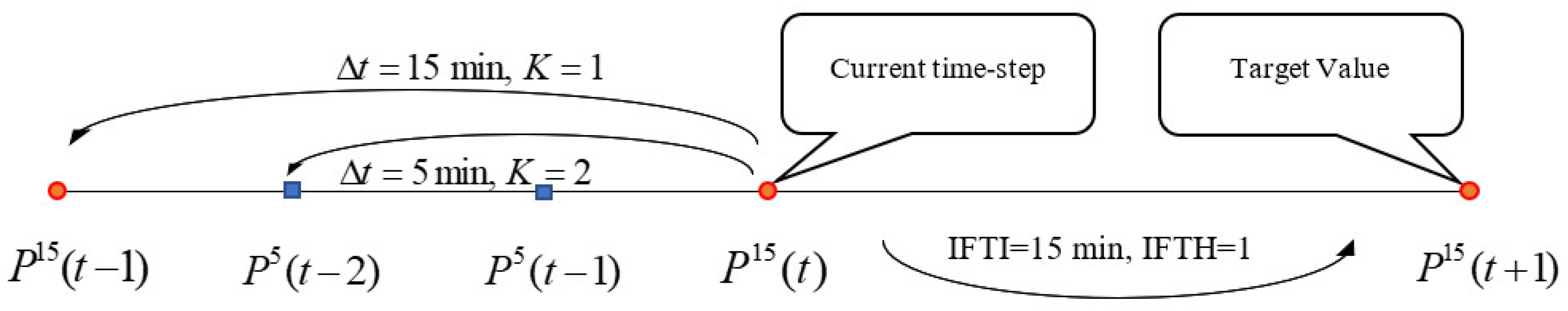
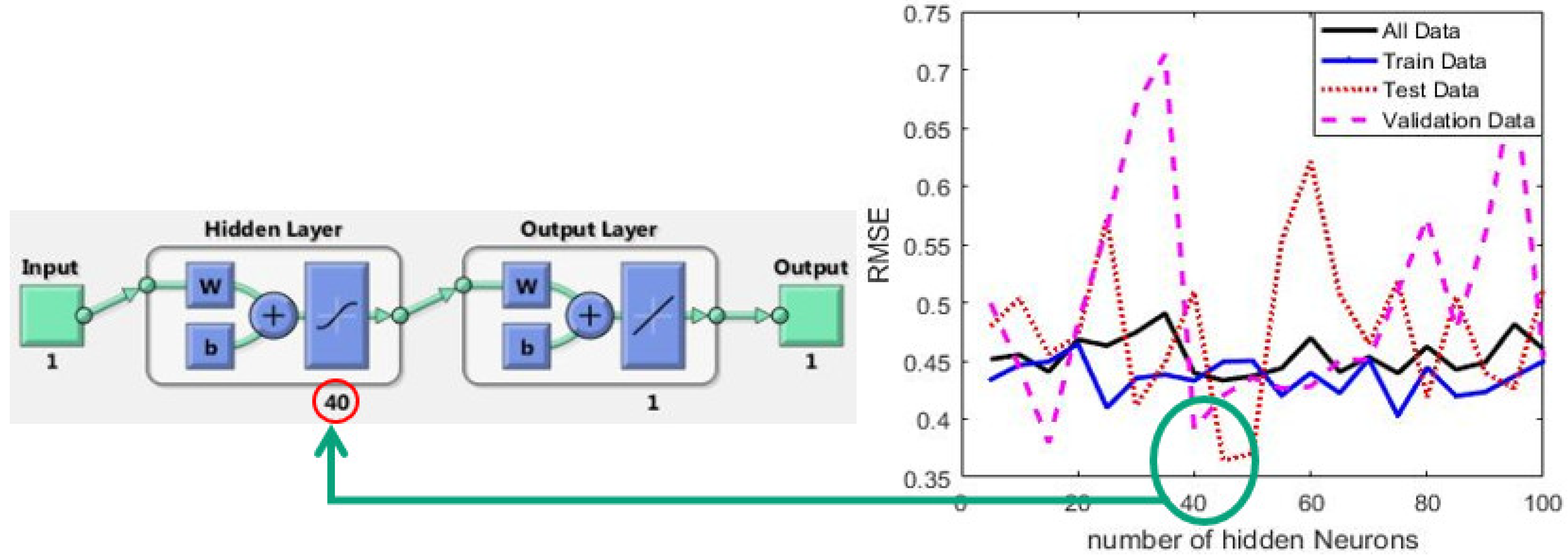
2.2. Short-Term Rainfall Prediction Model

Rainfall is a complicated atmospheric process that is influenced by a number of elements and their temporal-spatial patterns, including temperature, humidity, etc. An ANN model is utilized to predict the rainfall depth of a 15 min time period in which only the rainfall depths of previous time steps are available as predictor variables. In this study, the input forecasting time interval (IFTI) is 15 min, and the input forecast time horizon (IFTH) is 30 min, or twice the IFTI. In other words, the precipitation amounts for the next two 15 min intervals are forecasted. For the sake of forecasting, the incremental rainfall depth at a target point is analyzed as a function of a finite number of preceding observations as follows:
P ( t + 1 ) = f ( P ( t ) , P ( t 1 ) , P ( t 2 ) , , P ( t k + 1 ) ) + e ( t ) ,
where P t = the rainfall depth at the time t ; f ( ) = a nonlinear function that is going to be estimated by ANNs; K = the influential lag-time of the past rainfall realizations affecting the rainfall depth at the next time step; and e t = the ANN model’s forecast error to be minimized. It should be noted that the short-term rainfall prediction model described here is an adaptation of a non-linear autoregressive moving average model specifically designed for Artificial Neural Networks. This adaptation has been implemented to simplify the calibration process for the model.
In this study, a basic ANN configuration, i.e., Multi-layer Feedforward Neural Network (MLFNN), is used with the Levenberg-Marquardt training method [43]. For the hidden layer and output layer, respectively, the tan-sigmoid transfer function and a linear function are applied. Forecast accuracy is affected by the ideal number of hidden layers and neurons, which should be chosen depending on the nonlinearity level of the problem and the quantity and quality (precision) of available data [44]. The majority of complex continuous functions can be approximated by a single hidden layer [43,44]; hence, a single hidden layer was utilized, and 5 to 100 hidden neurons were evaluated.
Proper selection of the predictors is an important task that affects the performance of the ANN model. This is a concern based on the additional information each predictor would supply and the complexity of the ANN model (number of parameters). As expected, our investigations demonstrated that the first lag time (Lag-1) information was of the utmost value in the developed ANN models, as supported by other studies such as [41]. In other words, 15 min rainfall time series have characteristics of short-term memory [38]. Nonetheless, the substantial variability of rainfall hydrographs across time intervals smaller than 15 min was an additional element that prompted us to account for this variability. For this reason, a novel theory has also been evaluated, which focuses more on rainfall variations by incorporating difference-type variables and finer-resolution 5 min rainfall depths as supplementary predictors for 15 min rainfall depth forecasting. Hence, the following three scenarios with new sets of combinations of predictors are evaluated for forecasting the next 15 min rainfall depth, P 15 t + 1 :
Scenario   I :   P 15 t ,
Scenario   II :   P 15 t , P 15 t P 15 t 1 ,
and
Scenario   III :   P 15 t , P 5 t P 5 t 1 , P 5 t 1 P 5 t 2
where P Δ t t K is the rainfall depth with a Δ t minute time resolution (i.e., time interval) that occurred with K time-step delay from time-step t . The above scenarios are evaluated to forecast P 15 t + 1 which is the rainfall depth for one time step ahead (IFTH = 1), where IFTI = 15 min. For example, as shown in Figure 2, scenario III considers rainfall depth that occurred at previous 15 min time intervals and rainfall variations with a finer time resolution of 5 min intervals to predict rainfall depth for the next time step.
Prior to the training stage, it would be crucial to preprocess the data after selecting predictors. Data clustering using the K-means algorithm [45] and data normalization are two techniques used in this study. The range of all variables has been transferred first to [0–1] using Equation (2).
X i = x i x min x max x min , w h e r e x min = M i n x i , a n d x max = M a x x i
Common statistical parameters, including the coefficient of determination R 2 and root mean square error ( R M S E )   are used to decide on the best forecasting model with the highest FAC [46]. The dataset was randomly divided into 70, 15, and 15% as training, validation, and test datasets, respectively, and the model resulted in the least error with respect to the validation set selected.

2.3. Model Predictive Control Set-Up for Gate Regulation

A control gate is one of the actuators employed by urban drainage systems to effectively minimize the flood’s peak and volume. It helps regulate flows at the detention reservoir outlet in UDSs [27]. In this study, a PR-MPC strategy comprised of three linked modules, namely short-term rainfall forecasting, the SWMM rainfall-runoff internal model, and the HS optimizer, was presented to generate optimal operating policies for the regulation of detention tank gates.
Given a detention tank with an outflow gate located B meters above its bottom surface (Figure 3), the optimal operating rule curve as a result of the MPC strategy would be a vector of policies as [ G 1 , G 2 , G 3 , , G j , , G n ] , in which G j is the percentage of the gate opening corresponding to discrete water levels within the interval [ d j , d j + 1 ) . Height B affects the size of this vector n as the gate does not start working as long as the water level is below this height.
Real-time and predictive performance are the two major components of the proposed MPC architecture. In this model, the whole operation time horizon (24 h as the longest base time of flood events investigated) is divided into several sampling time intervals [ T i , T i + 1 ) (considered as 30 min herein), and a particular operating rule T i is generated corresponding to each sampling interval T i , where each R i is a G j vector. The control rule obtained is applied to the system during the current CTH. Hence, an ongoing operation over the operation time horizon leads to a finite sequence of operating policies [ R 1 , R 2 , , R i , , R H ] . Alternatively, using a predictive approach, the operating policies are derived from the available data, the present condition of the system, and the predicted future rainfalls, which are periodically updated for each sampling time based on the most recent data and the actual state of the system.
The optimization model that is solved at each sampling time interval is a multi-period model because the objective function, such as the total volume of the flood, is minimized over multiple time periods beginning with the current sampling time interval and ending with the end of the flood event, taking into account all physical and operational constraints, such as hydraulic rules and other operational system requirements. The formulation of the optimization model at the sampling time interval T i is as follows:
M I N :   T = T i T H F T
Subject to:
F T = f P ,   h t ,   G j ,   T i
h t = f h t 1 ,   Q i n ,   t ,   G j T i
0 h t H M A X
[ G j ] T i = 0                                                                           i f   h t B Z = 1 n d i s Z z × K z                                         o t h e r w i s e  
z = 1 n d i s Z z = 1 ,
where F t = the total flood volume during the PTH as a function of the rainfall hyetograph P containing observed and forecasted rainfall depths; G j = operating rule curve consisting of the decision variables of the optimization model and other system parameters and state variables that are determined by the SWMM simulation model, such as hydraulic properties and capacities of pipes, flow discharges, etc. Hydraulic and hydrologic equations solved by the simulation model are represented as constraints (4) to (6). ħ t   = water level in the detention tank at time t ( t refers to the time-step of the simulation model), which is a function of inflow discharge to the reservoir Q m , t , water level at the previous time-step, ħ t 1 , and G j . Equation (7) shows how the variables of the function G j are accounted for in the formulation, where K z = an integer variable whose value is specified from the vector [0, 10%, 20%, …, 100%] of n d i s = 11   size; and Z z = a binary variable.
At the beginning of each sampling interval, the aforementioned formulation is solved. Although the optimization problem is solved over the PTH, the acquired operating policy is only applied to the current CTH, and the procedure is repeated for each sampling time in the remaining future time intervals. Additionally, the rainfall hyetograph P is updated periodically at the beginning of each sampling time using the most recent observed data, and the rainfall forecasts are updated by the short-term forecasting model up to the IFTH.

2.4. Simulation-Optimization Model

The optimization problem provided in Section 2.2 is a mixed-integer nonlinear program (MINLP) that is solved by the meta-heuristic optimization algorithm Harmony Search (HS) introduced by Geem et al. [47]. The HS optimizer has been coupled with the internal SWMM simulator to provide an optimization-simulation modeling framework as a fundamental component of the proposed adaptive MPC strategy. The HS optimizer seeks the optimal values for decision variables, drawing inspiration from the musical process, wherein perfect harmony is determined through aesthetic judgment. The algorithm’s consecutive steps are as follows:
Step 1: The harmony memory matrix H M is filled by the number of random vectors ( x 1 , x 2 , x 3 ,   , x H M S )   equal to the determined harmony memory size H M S as shown in Equation (9).
H M = x 1 1 x n 1 x 1 h m s x n h m s | | | f x 1 f x h m s
Step 2: A set of new harmonies x as many as the repository size (RS) are generated and stored in the repository with the probability H M C R as the harmony memory considering whose value is selected from predefined H M :   x i x i int ( u ( 0 , 1 ) × H M S ) + 1 ; and is specified randomly otherwise with the probability 1 H M C R .
Step 3: If x in Step 2 is selected from the H M , then an additional procedure will be required as follows:
x is modified slightly through parameter δ as ( x i x i δ ) with probability 0     PAR     1 called the pitch adjusting rate; otherwise, no modification will be performed with the probability of 1 PAR .
Step 4: The harmony memory ( H M ) and repository are merged and sorted according to objective function values. The new H M matrix is updated, including the first best harmonies and as many as H M S .
Step 5: Steps 2 to 4 are repeated until the termination criterion is satisfied. The criterion is chosen based on either finding a solution corresponding to a zero flood volume, exceeding the maximum allowable number of function evaluations, or no change in the best solution found over 50 consecutive iterations.
In the HS algorithm, a new solution vector is generated considering the whole existing solutions stored in the H M matrix based on parameters H M C R and P A R , whereas only two parent solutions are used for the evolution of solutions in, for example, GA. This feature increases the performance of the HS algorithm in finding global optima [48].

3. Study Area

To test the performance of the proposed model, it is applied to a drainage system located in the southern portion of the major UDS of Tehran, Iran, which consists of 42 subcatchments and 132 conduits and covers an area of 156 km 3 . The system fails to properly transport stormwater runoff from a rainfall event with a 50-year return period because approximately 15.6 of 116 km underground tunnels do not have sufficient capacity for the subsequent flood. North and South Saleh Abad, two detention reservoirs connected by a central culvert, have been added to the system to increase its storage capacity. Based on their similar hydraulic performance, one equivalent detention tank with a maximum capacity of 62.5 × 10 3   m 3   is considered in this analysis [32].
Figure 4 depicts the Tehran central basin and the drainage network in the associated SWMM simulation model, including a concrete outlet intake structure equipped with three steel sluice gates of 1 .6 × 1.6   m   size, eight rectangular openings of 0 .6 × 0.9   m dimension at the upper part, and a three-diameter octagonal opening on the roof of the structure that acts as a spillway when the water level rises. The optimal operation of these gates and openings is sought in an effort to mitigate the effects of flooding.

SWMM Model Inputs

For the development of a short-term rainfall prediction model, meteorological gauges in the study area are utilized to record observed rainfall events at 1 5   min and 5   min intervals from 1973 to 2014. There are a total of 335 precipitation occurrences, with depths and durations ranging from 0.1 to 61.5 mm and 15 to 2235 min, respectively (Figure 5). After excluding zero values, the total number of datapoints for the time series extracted at 15 min intervals is 8063.
According to Table 1, six events are chosen to assess the performance of the produced models, such as the rainfall forecasting model and the RE- and PR-MPC models. These events encompass a variety of rainfall depth and duration ranges, as well as hydrologic process variations.

4. Numerical Experiments and Results

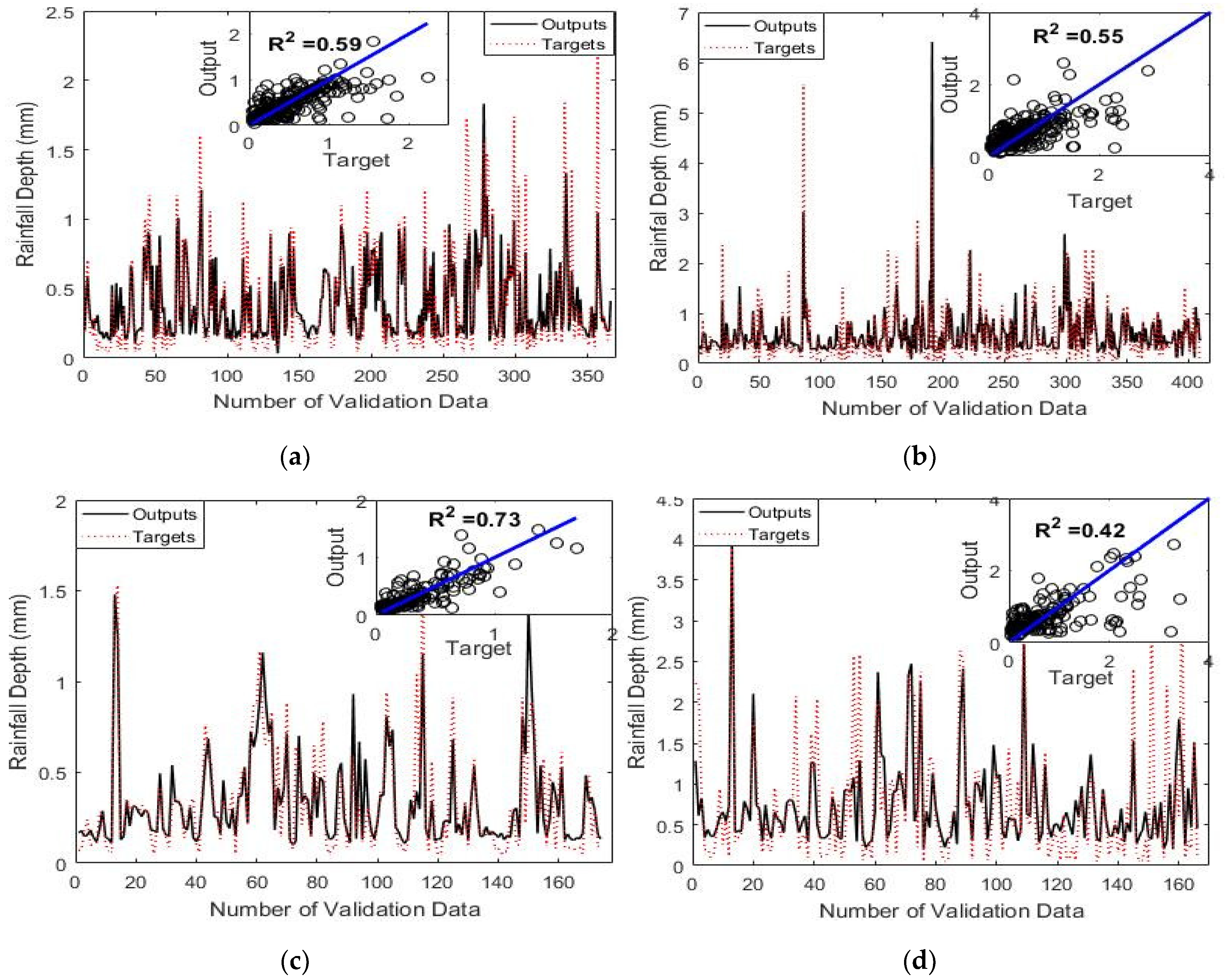
4.1. Results of Short-Term Rainfall Forecasting

Figure 6 depicts the layout of the ANN model and the processes used to determine the appropriate number of neurons in the hidden layer corresponding to the first set of predictors, where the only predictor is the rainfall depth of the previous time step.
To improve the forecast accuracy, 335 total rainfall events were classified into four clusters using the K-means algorithm [50] based on the two main aspects of the events, i.e., depth and duration, as shown in Table 2.
As described in Section 2.1, three sets of predictors (scenarios) were evaluated to establish the optimal combination of predictors. Table 3 displays the outcomes of the scenarios applied to several datasets, including the complete 8063 data set and the data classes C1, C2, C3, and C4 separately. According to the results, scenario III improved forecast accuracy by as much as 40 percent compared with the other two scenarios. In other words, in addition to the rainfall depth for the preceding time step, incorporating its fluctuations across finer 5 min resolutions significantly enhances the effectiveness of the forecast model. The lowest-accuracy cluster is C4, which contains the most intense and unpredictable rainfall pulses. However, from the perspective of flood control, these rainfall events are less significant due to their shorter durations and shallower depths, which make them easier to manage even without knowledge of future precipitation. In scenario III, Figure 7 compares the observed and predicted values corresponding to various classes. In the proposed MPC framework, these four forecasting models will be used. Although forecast accuracies are not particularly high, they are comparable with the findings of earlier experiences reported for short-term rainfall forecasting; see, for instance, [38,41]. In addition, it is essential to determine if such levels of forecast precision may still improve the performance of the RTC of urban drainage systems. In the next section, the performance of the PR-MPC is compared with that of the RE-MPC.
Using the best ANN forecasting model (model of scenario III) to predict the next two time steps ( P 15 t + 1 ) resulted to R 2 equal to 0.31, 0.29, 0.34, and 0.14 for clusters C1, C2, C3, and C4, respectively.

4.2. Results of the MPC Framework

According to Table 2, Class C4 is comprised of the events with the shortest average duration and depth, as shown in Figure 8a, which is a histogram of rainfall depth. In Class C4, the average precipitation depth is approximately 7.5 mm, and the total precipitation depth for almost all events is less than 20 mm. Applying the RE-MPC model [24] to four sample C4 events, namely events 1, 2, 4, and 6, without knowledge of future rainfall data revealed that the RE-MPC approach could manage these events without any flooding while not even the entire storage capacity of the detention reservoir was utilized (Figure 8b).
Therefore, advanced warning of future precipitation (i.e., employing the PR-MPC technique) would be more beneficial for occurrences with longer durations and greater intensities that belong to the other three groups. This result is similar to the findings of prior research in this field, as in [9]. indicated that the benefits of the RTC technique become more substantial for events lasting more than two hours [9].
Information and data are exchanged between the simulation, optimization, and rainfall forecasting modules in accordance with the PR-MPC system depicted in Figure 1. The linked HS-SWMM optimization-simulation model uses the same parameter adjustment and setup approach as [24] for a reactive real-time optimal control model.
Four types of rainfall forecasting models have been created to predict rainfall depths two time steps in advance. At the start of a storm event, there is insufficient information to determine which of the four forecast models would be the most accurate for the actual event. In practice, however, an adaptive approach is necessary to identify and link the optimal forecast model to the coupled HS-SWMM framework. In the first sampling interval, the average outputs of the four forecast models are used for this purpose, and the forecast errors for each model are determined using the actual rainfall pulse. For succeeding time intervals, the forecasting model with the smallest error across the preceding time steps will be utilized. Using this method, the optimal forecast model would be detected adaptively after a few time steps.
According to Table 4, five distinct MPC-based models are built, based on the varied IFAC and IFTH, to examine the impact of the input forecast module on the RTC of UDSs and the efficacy of the PR-MPC technique over the RE-MPC method.
Models A and B are PR-MPC models that benefit from the perfect input forecast, assuming no forecast error (IFAC = 100%) and having an IFTH equal to the entire duration of the rainfall event (i.e., complete information regarding future rainfalls) and two 15 min time steps (i.e., complete information regarding a subset of future rainfalls), respectively. These models disregard the forecast uncertainty that represents the best possible ideal circumstance, but they address two distinct conditions regarding the extent (duration) of perfect knowledge of future rainfalls. Models C and D represent the proposed PR-MPC framework employing the developed forecast module with IFTH values of two and one 15 min time increment, respectively. Model E is the RE-MPC that utilizes only the current available precipitation data and has no knowledge of future precipitation. Table 5 compares the efficiency of the examined models for two storm occurrences, events 3 and 5, belonging to the first and second clusters, respectively (Table 1).
The results reveal that, compared with the RE-MPC model, Model A, as an ideal but unrealistic model, has resulted in flood volume reductions of 25% and 10%, respectively, for events 5 and 3. Using the available storage capacity and drainage system characteristics, Model A’s global optimal solution is the best theoretical solution that can ever be attained. Model B results in flood volume increases of 10% and 6% for events 5 and 3, respectively, when compared with Model A, due to its reduced IFTH (knowing less about the future) when forecasts have still been error-free. Model C has the same IFTH as Model B, but according to the best ANN forecasting model developed, the used forecasts are imprecise. As expected, the decrease in forecast accuracy (IFAC) has caused the flood volume for events 5 and 3 to increase by 4.0% and 2.3% relative to Model B, respectively. Despite having the same IFAC, Model D performed around 9% and 4% worse than Model C for events 5 and 3, respectively, because of using a shorter IFTH given the IFAC of the best ANN model. Therefore, IFAC and IFTH each contribute to the performance of the PR-MPC models. The longer the forecast lead time, the lower the IFAC will be. Importantly, the proposed PR-MPC model (Model C) has achieved approximately 85% and 92% of the performance of the best solutions that can ever be found (Model A’s ideal solutions) for events 5 and 3, respectively, based on the findings of the various models shown in Table 5. Using Equation (10) to quantify forecast error, the average errors obtained for one time step ahead (IFTH = 1) forecasts for events 3 and 5 are 0.28 and 0.53, while those errors for the next two time step forecasts (IFTH = 2) are 0.44 and 0.64 for the same events.
e i = x r e f i x i x r e f i 0
where x i and x r e f i refer to forecasted and observed values, respectively.
In Model A, by assuming perfect, error-free forecasts, x i = x r e f i , the value of prediction error is ( x r e f i x r e f i x r e f i = 0 ) ; whereas in Model E, in which no rainfall forecasts are used, it is like x i = 0 , so the error is equal to ( x r e f i 0 x r e f i = 1 ) . Depending on the current condition of the system, the forecast lead time, and the IFAC of the ANN rainfall forecast model, the forecast error for the PR-MPC model can range from 0 to a huge value of M. Theoretically, having information and knowledge about future rainfalls would have a favorable effect on the PR-MPC model as long as the forecast mistakes are not so large that the model that ignores these errors (Model E) performs better than the model that incorporates them (Models B and C). Consequently, an effective IFTH is a time horizon under which the associated PR-MPC model outperforms a RE-MPC. The longer the effective IFTH is, the more accurate the forecast model will be. As depicted in Figure 9 for events 5 and 3, the system is susceptible to multiple small early floods if Model A’s operations are implemented; hence, this model manages system operations to limit peak flows and flood volumes. Model C has followed Model A’s ideal operations very well; however, Model E has not.
Figure 10 depicts the observed and predicted rainfall hyetographs for the two analyzed rainfall events. Model C forecasts precipitation amounts during two consecutive time steps (IFTH = 2). In other words, for each 30 min sampling interval, in addition to the updated realized rainfall depths up to the present time step, two predicted values of rainfall depth for the subsequent 15 and 30 min are also employed to determine appropriate operation policies for the current time period. The graph illustrates that bigger forecast errors correspond to the hyetograph’s extremum spots.
Apart from forecasting errors and variations, the model’s adaptability to forecast errors makes the performance of the proposed adaptive PR-MPC framework more appealing. Figure 11 demonstrates how well the adaptive mechanism employed in this model performs over time for the two investigated events. It illustrates differences in the primary characteristics of flood events, such as total flood volume, flood peak discharge, and time to peak, throughout successive sampling time intervals ( T i ) of the operation horizon in comparison with Model A’s perfect solution. Observers will note that as time passes and more information is gathered, Model C’s outcome steadily approaches that of Model A. This clearly demonstrates the benefit of updating optimal policies adaptively throughout each sampling interval in the PR-MPC model.

5. Final Remarks

Developing and planning a RTC model for the operation of an UDS is a complex process that necessitates additional effort and cost for the instrumentation of the facilities, including software and hardware technologies, mechanical equipment, measurement devices, local stations, communications, a meteorological forecasting system, and maintenance [33]. In contrast, RTC approaches have dramatically increased the adaptability and flexibility of the system’s operations in response to varied rainfall load scenarios [51]. In addition, it saves money by activating the existing storage capacity without the need to build additional retention volume [16]. Therefore, the RTC approach should be considered for UDSs’ operations management as it offers meaningful benefits to the environment, system operators, and stakeholders exposed to charges [16]. Dresden (Germany), Vienna (Austria), and Quebec (Canada) are places where RTC systems have been successfully implemented in urban wastewater systems [52,53,54].
Dresden and Vienna also use the same RTC system, which consists of a simplified coarse network of the cities′ sewer systems simulated in the HYSTEM-EXTRAN rainfall-runoff model, a rule interpreter software called ITWH-CONTROL to make control decisions based on the if-then rules and fuzzy logic, and a rainfall forecast module employing the “tracking method” [53]. A predictive RTC system manages the sewer system of Quebec City, which includes a linear input-output moving average simulation model, a nonlinear optimization algorithm, and the CALAMAR radar-based rainfall forecast model [33]. The predicted rainfall intensities using CALAMAR were reported as 30% of the actual data [33].
The aforementioned RTC systems simplify the hydraulic simulation model of the studied areas to maintain the optimization computation time within an appropriate applicable range while increasing the related simulation model uncertainty. In contrast, the proposed PR-MPC framework reduces the simulation model uncertainty by employing the original SWMM simulation model of the study area, consisting of 42 sub-catchments and 132 conduits, directly linked to the optimization module. However, the underlying simulation model is separated into two upstream and downstream sub-models to circumvent the runtime limitation. During each sample interval, the upstream sub-model is executed only once to compute its outflow, which is then utilized as the inflow to the downstream sub-model. Therefore, only the downstream model is called for each objective function evaluation; consequently, the entire optimization process takes approximately 13 min on a system with an Intel Core i7 processor running at 3.2 GHz and 16 GB of RAM. This strategy is based on the fact that the upstream sub-model establishes gravity flow irrespective of the operation of the downstream gates, as discussed and confirmed in [7] and [24].
The rainfall forecast module is another distinction between the proposed model and those proposed previously, as it employs an ANN-based rainfall forecast model with adaptive performance and better accuracy for short-term rainfall forecasting using a novel mix of predictors. Last but not least, this study compares the two MPC approaches of RE-MPC and PR-MPC, showing the outperformance of the PR-MPC approach over the RE-MPC model. However, this advantage is more apparent for longer-period rainfall events that place a greater load on the system than its capacity. There is also a trade-off between IFTH and IFAC, so the best rainfall IFTH can be determined based on the resulting IFAC.

6. Conclusions

In this study, the K-means clustering algorithm was used to evaluate the short-term (up to 30 min ahead) rainfall forecast precision and its impact on urban flood control operations for a variety of rainfall patterns in terms of depth and duration. A predictive MPC (PR-MPC) framework was developed to evaluate the role of rainfall forecast features and accuracy in flood management and operations of a part of Tehran’s urban drainage system, Iran, by deriving optimal operation policies for the system’s gate regulation. Five distinct operational models were examined with respect to their input forecast time horizon (IFTH) and accuracy (IFAC), including: (a) a zero-IFTH reactive MPC (RE-MPC) model to a model IFTH of which was the entire rainfall duration (Model A); and (b) models benefiting from perfect, error-free forecasts (Models A and B) to those utilizing data-clustered ANN-based forecasting models developed based on actual historical rainfall events (Models C and D). Additionally, the best-fit ANN forecasting model for a particular event was found adaptively after a few time steps of the PR-MPC operation. The results and contrasts revealed:
  • Clustering rainfall data as a preprocessing technique not only increased the accuracy of precipitation forecasts but also the performance of the adaptive forecast-based PR-MPC operation model. This suggests that utilizing clustering algorithms can be beneficial in improving forecast precision for flood management.
  • The accuracy of ANN forecast models was enhanced by the addition of predictors describing variations in rainfall depth over shorter time intervals than the forecast lead time. This indicates that capturing short-term variations in rainfall depth can contribute to more accurate forecasts.
  • The rainfall forecasting module showed a higher impact on the performance of the PR-MPC operation strategy for longer-duration, larger-magnitude rainfall events. This highlights the importance of accurate rainfall forecasts in optimizing flood control operations, particularly for more heavy rainfall events.
  • Despite inaccuracies in rainfall forecasts and the ANN model’s uncertainty, the forecast-based adaptive PR-MPC operation model performed 11% better in terms of flood volume reduction than the RE-MPC operation model that did not use rainfall forecasts. This accomplishment was partially attributed to the adaptively updating ANN-based rainfall forecasts and the PR-MPC operating model’s control rules over a dynamic, uncertain decision-making process.
The significance of these findings lies in their implications for urban flood control operations and the potential for improving flood management strategies. The study provides evidence that incorporating accurate and adaptive rainfall forecasting models into the PR-MPC framework can lead to significant improvements in flood volume reduction. Future research in this field should focus on reducing predictive model uncertainty by integrating more precise rainfall forecast modules into the proposed PR-MPC framework. This could further enhance the effectiveness of flood control operations and contribute to more resilient urban drainage systems.

Author Contributions

S.J.M., F.J. and K.P. developed and proposed the main ideas behind this paper. F.J. performed the required coding and computer implementation and wrote the first draft. All authors have read and agreed to the published version of the manuscript.

Funding

This research received no external funding.

Data Availability Statement

The data presented in this study are available on request from the corresponding author.

Acknowledgments

The authors thank Jafar Yazdi for providing us with the data for the case study and his recommendations.

Conflicts of Interest

The authors declare no conflict of interest.

Abbreviations

ANNartificial neural networks
CTHcontrol time horizon
FACforecast accuracy
GAgenetic algorithm
HMharmony memory matrix
HMCRharmony memory considering rate
HMSharmony memory size
HSharmony search
IFACinput (rainfall) forecast accuracy
IFTHinput (rainfall) forecast time horizon
MINLPmixed-integer nonlinear program
MLFNNMulti-layer Feedforward Neural Network
MPCmodel predictive control
PARpitch adjusting rate
PR-MPCpredictive MPC
PTHprediction time horizon
RE-MPCreactive MPC
RSrepository size
RTCreal-time control
SWMMstorm water management model
Tisampling time intervals
UDSurban drainage systems

References

  1. Luo, P.; He, B.; Takara, K.; Xiong, Y.E.; Nover, D.; Duan, W.; Fukushi, K. Historical assessment of Chinese and Japanese flood management policies and implications for managing future floods. Environ. Sci. Policy 2015, 48, 265–277. [Google Scholar] [CrossRef] [Green Version]
  2. Zhang, X.; Peng, Y.; Xu, W.; Wang, B. An Optimal Operation Model for Hydropower Stations Considering Inflow Forecasts with Different Lead-Times. Water Resour. Manag. 2018, 33, 173–188. [Google Scholar] [CrossRef]
  3. Babovic, F.; Mijic, A.; Madani, K. Decision making under deep uncertainty for adapting urban drainage systems to change. Urban Water J. 2018, 15, 552–560. [Google Scholar] [CrossRef]
  4. Ferdous, R.; Di Baldassarre, G.; Brandimarte, L.; Wesselink, A. The interplay between structural flood protection, population density, and flood mortality along the Jamuna River, Bangladesh. Reg. Environ. Chang. 2020, 20, 5. [Google Scholar] [CrossRef] [Green Version]
  5. Todeschini, S.; Papiri, S.; Ciaponi, C. Performance of stormwater detention tanks for urban drainage systems in northern Italy. J. Environ. Manag. 2012, 101, 33–45. [Google Scholar] [CrossRef]
  6. García, L.; Barreiro-Gomez, J.; Escobar, E.; Téllez, D.; Quijano, N.; Ocampo-Martinez, C. Modeling and real-time control of urban drainage systems: A review. Adv. Water Resour. 2015, 85, 120–132. [Google Scholar] [CrossRef] [Green Version]
  7. Jafari, F.; Mousavi, S.J.; Yazdi, J.; Kim, J.H. Real-Time Operation of Pumping Systems for Urban Flood Mitigation: Single-Period vs. Multi-Period Optimization. Water Resour. Manag. 2018, 32, 4643–4660. [Google Scholar] [CrossRef]
  8. Lund, N.S.V.; Falk, A.K.V.; Borup, M.; Madsen, H.; Mikkelsen, P.S. Model predictive control of urban drainage systems: A review and perspective towards smart real-time water management. Crit. Rev. Environ. Sci. Technol. 2018, 48, 279–339. [Google Scholar] [CrossRef]
  9. Mullapudi, A.; Lewis, M.J.; Gruden, C.L.; Kerkez, B. Deep reinforcement learning for the real time control of stormwater systems. Adv. Water Resour. 2020, 140, 103600. [Google Scholar] [CrossRef]
  10. Ocampo-Martinez, C. Model Predictive Control of Wastewater Systems; Springer: London, UK, 2010. [Google Scholar] [CrossRef]
  11. van der Werf, J.A.; Kapelan, Z.; Langeveld, J. Quantifying the true potential of Real Time Control in urban drainage systems. Urban Water J. 2021, 18, 873–884. [Google Scholar] [CrossRef]
  12. Hooshyar, M.; Mousavi, S.J.; Mahootchi, M.; Ponnambalam, K. Aggregation–Decomposition-Based Multi-Agent Reinforcement Learning for Multi-Reservoir Operations Optimization. Water 2020, 12, 2688. [Google Scholar] [CrossRef]
  13. Mousavi, S.J.; Ponnambalam, K.; Celeste, A.B.; Cai, X. Enhancements to explicit stochastic reservoir operation optimization method. Adv. Water Resour. 2022, 169, 104307. [Google Scholar] [CrossRef]
  14. Yu, P.-S.; Yang, T.-C.; Chen, S.-Y.; Kuo, C.-M.; Tseng, H.-W. Comparison of random forests and support vector machine for real-time radar-derived rainfall forecasting. J. Hydrol. 2017, 552, 92–104. [Google Scholar] [CrossRef]
  15. Kerkez, B.; Gruden, C.; Lewis, M.; Montestruque, L.; Quigley, M.; Wong, B.; Bedig, A.; Kertesz, R.; Braun, T.; Cadwalader, O.; et al. Smarter Stormwater Systems. Environ. Sci. Technol. 2016, 50, 7267–7273. [Google Scholar] [CrossRef] [Green Version]
  16. Beeneken, T.; Erbe, V.; Messmer, A.; Reder, C.; Rohlfing, R.; Scheer, M.; Schuetze, M.; Schumacher, B.; Weilandt, M.; Weyand, M. Real time control (RTC) of urban drainage systems—A discussion of the additional efforts compared to conventionally operated systems. Urban Water J. 2013, 10, 293–299. [Google Scholar] [CrossRef]
  17. Borsányi, P.; Benedetti, L.; Dirckx, G.; De Keyser, W.; Muschalla, D.; Solvi, A.-M.; Vandenberghe, V.; Weyand, M.; Vanrolleghem, P.A. Modelling real-time control options on virtual sewer systems. J. Environ. Eng. Sci. 2008, 7, 395–410. [Google Scholar] [CrossRef]
  18. Cembellín, A.; Francisco, M.; Vega, P. Distributed Model Predictive Control Applied to a Sewer System. Processes 2020, 8, 1595. [Google Scholar] [CrossRef]
  19. Chang, L.-C.; Chang, F.-J.; Hsu, H.-C. Real-Time Reservoir Operation for Flood Control Using Artificial Intelligent Techniques. Int. J. Nonlinear Sci. Numer. Simul. 2010, 11, 887–902. [Google Scholar] [CrossRef]
  20. Chiang, Y.-M.; Chang, L.-C.; Tsai, M.-J.; Wang, Y.-F.; Chang, F.-J. Auto-control of pumping operations in sewerage systems by rule-based fuzzy neural networks. Hydrol. Earth Syst. Sci. 2011, 15, 185–196. [Google Scholar] [CrossRef] [Green Version]
  21. Darsono, S.; Labadie, J.W. Neural-optimal control algorithm for real-time regulation of in-line storage in combined sewer systems. Environ. Model. Softw. 2007, 22, 1349–1361. [Google Scholar] [CrossRef]
  22. Garofalo, G.; Giordano, A.; Piro, P.; Spezzano, G.; Vinci, A. A distributed real-time approach for mitigating CSO and flooding in urban drainage systems. J. Netw. Comput. Appl. 2017, 78, 30–42. [Google Scholar] [CrossRef]
  23. Hsu, N.-S.; Huang, C.-L.; Wei, C.-C. Intelligent real-time operation of a pumping station for an urban drainage system. J. Hydrol. 2013, 489, 85–97. [Google Scholar] [CrossRef]
  24. Jafari, F.; Mousavi, S.J.; Yazdi, J.; Kim, J.H. Long-term versus Real-time Optimal Operation for Gate Regulation during Flood in Urban Drainage Systems. Urban Water J. 2018, 15, 750–759. [Google Scholar] [CrossRef]
  25. Maiolo, M.; Palermo, S.A.; Brusco, A.C.; Pirouz, B.; Turco, M.; Vinci, A.; Spezzano, G.; Piro, P. On the Use of a Real-Time Control Approach for Urban Stormwater Management. Water 2020, 12, 2842. [Google Scholar] [CrossRef]
  26. Rai, P.K.; Dhanya, C.T.; Chahar, B.R. Flood control in an urban drainage system using a linear controller. Water Pract. Technol. 2017, 12, 942–952. [Google Scholar] [CrossRef]
  27. Schütze, M.; Campisano, A.; Colas, H.; Schilling, W.; Vanrolleghem, P.A. Real-time control of urban wastewater systems—Where do we stand today? J. Hydrol. 2004, 299, 335–348. [Google Scholar] [CrossRef]
  28. Sun, C.; Svensen, J.L.; Borup, M.; Puig, V.; Cembrano, G.; Vezzaro, L. An MPC-Enabled SWMM Implementation of the Astlingen RTC Benchmarking Network. Water 2020, 12, 1034. [Google Scholar] [CrossRef] [Green Version]
  29. Wei, C.-C.; Hsu, N.-S.; Huang, C.-L. Two-Stage Pumping Control Model for Flood Mitigation in Inundated Urban Drainage Basins. Water Resour. Manag. 2013, 28, 425–444. [Google Scholar] [CrossRef]
  30. Yazdi, J.; Kim, J.H. Intelligent Pump Operation and River Diversion Systems for Urban Storm Management. J. Hydrol. Eng. 2015, 20, 04015031. [Google Scholar] [CrossRef]
  31. Chiang, P.-K.; Willems, P. Combine Evolutionary Optimization with Model Predictive Control in Real-time Flood Control of a River System. Water Resour. Manag. 2015, 29, 2527–2542. [Google Scholar] [CrossRef]
  32. Jafari, F.; Mousavi, S.J.; Kim, J.H. Investigation of Rainfall Forecast System Characteristics in Real-Time Optimal Operation of Urban Drainage Systems. Water Resour. Manag. 2020, 34, 1773–1787. [Google Scholar] [CrossRef]
  33. Pleau, M.; Colas, H.; Lavallée, P.; Pelletier, G.; Bonin, R. Global optimal real-time control of the Quebec urban drainage system. Environ. Model. Softw. 2005, 20, 401–413. [Google Scholar] [CrossRef]
  34. van Overloop, P.-J.; Weijs, S.; Dijkstra, S. Multiple Model Predictive Control on a drainage canal system. Control Eng. Pract. 2008, 16, 531–540. [Google Scholar] [CrossRef]
  35. Abraham, A.; Philip, N.S.; Joseph, K.B. Will We Have a Wet Summer? Soft Computing Models for Long Term Rainfall Forecasting. In Proceedings of the 15th European Simulation Multiconference (ESM 2001), Modelling and Simulation, Prague, Czechia, 6–9 June 2001; pp. 1044–1048. [Google Scholar]
  36. Wahyuni, E.G.; Fauzan LM, F.; Abriyani, F.; Muchlis, N.F.; Ulfa, M. Rainfall Prediction with Backpropagation Method. J. Phys. Conf. Ser. 2018, 983, 012059. [Google Scholar] [CrossRef]
  37. Lettenmaier, D.P.; Wood, E.F. Hydrologic Forecasting. In Handbook of Hydrology; Maidment, D.R., Ed.; McGraw-Hill: New York, NY, USA, 1993; Chapter 26. [Google Scholar]
  38. Luk, K.; Ball, J.; Sharma, A. A study of optimal model lag and spatial inputs to artificial neural network for rainfall forecasting. J. Hydrol. 2000, 227, 56–65. [Google Scholar] [CrossRef]
  39. Luk, K.C.; Ball, J.; Sharma, A. An application of artificial neural networks for rainfall forecasting. Math. Comput. Model. 2001, 33, 683–693. [Google Scholar] [CrossRef]
  40. Christodoulou, C.I.; Michaelides, S.C.; Gabella, M.; Pattichis, C.S. Prediction of rainfall rate based on weather radar measurements. In Proceedings of the 2004 IEEE International Joint Conference on Neural Networks (IEEE Cat. No. 04CH37541), Budapest, Hungary, 25–29 July 2004; IEEE: Piscataway, NJ, USA, 2004; Volume 2, pp. 1393–1396. [Google Scholar]
  41. Nasseri, M.; Asghari, K.; Abedini, M. Optimized scenario for rainfall forecasting using genetic algorithm coupled with artificial neural network. Expert Syst. Appl. 2008, 35, 1415–1421. [Google Scholar] [CrossRef]
  42. Adaryani, F.R.; Mousavi, S.J.; Jafari, F. Short-term rainfall forecasting using machine learning-based approaches of PSO-SVR, LSTM and CNN. J. Hydrol. 2022, 614, 128463. [Google Scholar] [CrossRef]
  43. Hagan, M.T.; Menhaj, M.B. Training feed-forward networks with the Marquardt algorithm. IEEE Trans. Neural Netw. 1994, 5, 989–993. [Google Scholar] [CrossRef]
  44. Reusch, D.B.; Alley, R.B. Automatic Weather Stations and Artificial Neural Networks: Improving the Instrumental Record in West Antarctica. Mon. Weather. Rev. 2002, 130, 3037–3053. [Google Scholar] [CrossRef]
  45. Hartigan, J.A. Clustering Algorithms; John Wiley & Sons Inc.: Hoboken, NJ, USA, 1975. [Google Scholar]
  46. Stanski, H.R.; Wilson, L.; Burrows, W.R. Survey of Common Verification in Meteorology; World Weather Watch Report 358; World Meteorological Organization: Geneva, Switzerland, 1989. [Google Scholar]
  47. Geem, Z.W.; Kim, J.H.; Loganathan, G.V. A new heuristic optimization algorithm: Harmony search. Simulation 2001, 76, 60–68. [Google Scholar] [CrossRef]
  48. Lee, K.S.; Geem, Z.W. A new meta-heuristic algorithm for continuous engineering optimization: Harmony search theory and practice. Comput. Methods Appl. Mech. Eng. 2005, 194, 3902–3933. [Google Scholar] [CrossRef]
  49. MGCE. Tehran Stormwater Management Master Plan. In Vol 4: Existing Main Drainage Network, Part 2: Hydraulic Modeling and Capacity Assessment, December 2011; MG Consultant Engineers, Technical and development deputy of Tehran municipality: Tehran, Iran, 2011. [Google Scholar]
  50. Bock, H.H. Clustering Methods: A History of k-Means Algorithms. In Selected Contributions in Data Analysis and Classification; Springer: Berlin/Heidelberg, Germany, 2007; pp. 161–172. [Google Scholar]
  51. Dirckx, G.; Schütze, M.; Kroll, S.; Thoeye, C.; De Gueldre, G.; Van De Steene, B. RTC versus static solutions to mitigate CSO’s impact. In Proceedings of the 12nd International Conference on Urban Drainage, Porto Alegre, Brazil, 11–16 September 2011. [Google Scholar]
  52. Fuchs, L.; Beeneken, T. Development and implementation of a real-time control strategy for the sewer system of the city of Vienna. Water Sci. Technol. 2005, 52, 187–194. [Google Scholar] [CrossRef] [PubMed]
  53. Fuchs, L.; Günther, H.; Lindenberg, M. Minimizing the Water Pollution Load by means of Real-Time Control (RTC)-The Dresden exemple. In Proceedings of the 6th International Conference on Urban Drainage Modelling, Dresden, Germany, 15–17 September 2004; pp. 317–325. [Google Scholar]
  54. Pleau, M.; Fradet, O.; Colas, H.; Marcoux, C. Giving the rivers back to the public. Ten years of real time control in Quebec city. In Proceedings of the NOVATECH 7th International Conference: Sustainable Techniques and Strategies in Urban Waste Water, Lyon, France, 27 June–1 July 2010; Available online: http://documents.irevues.inist.fr/bitstream/handle/2042/35732/31805-055ple.pdf?sequence=1 (accessed on 16 May 2023).
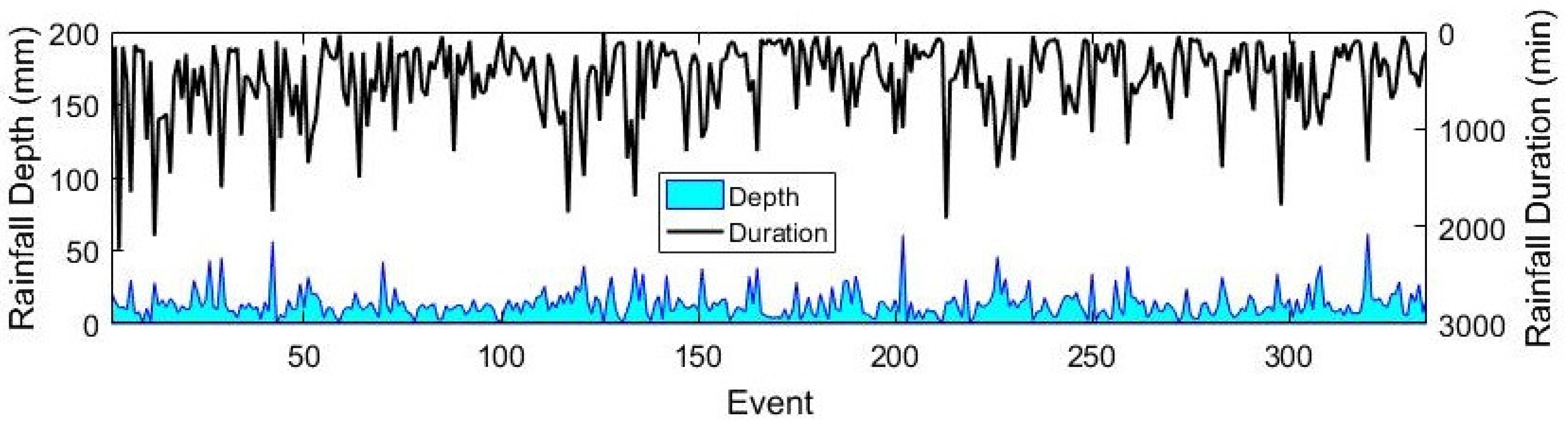
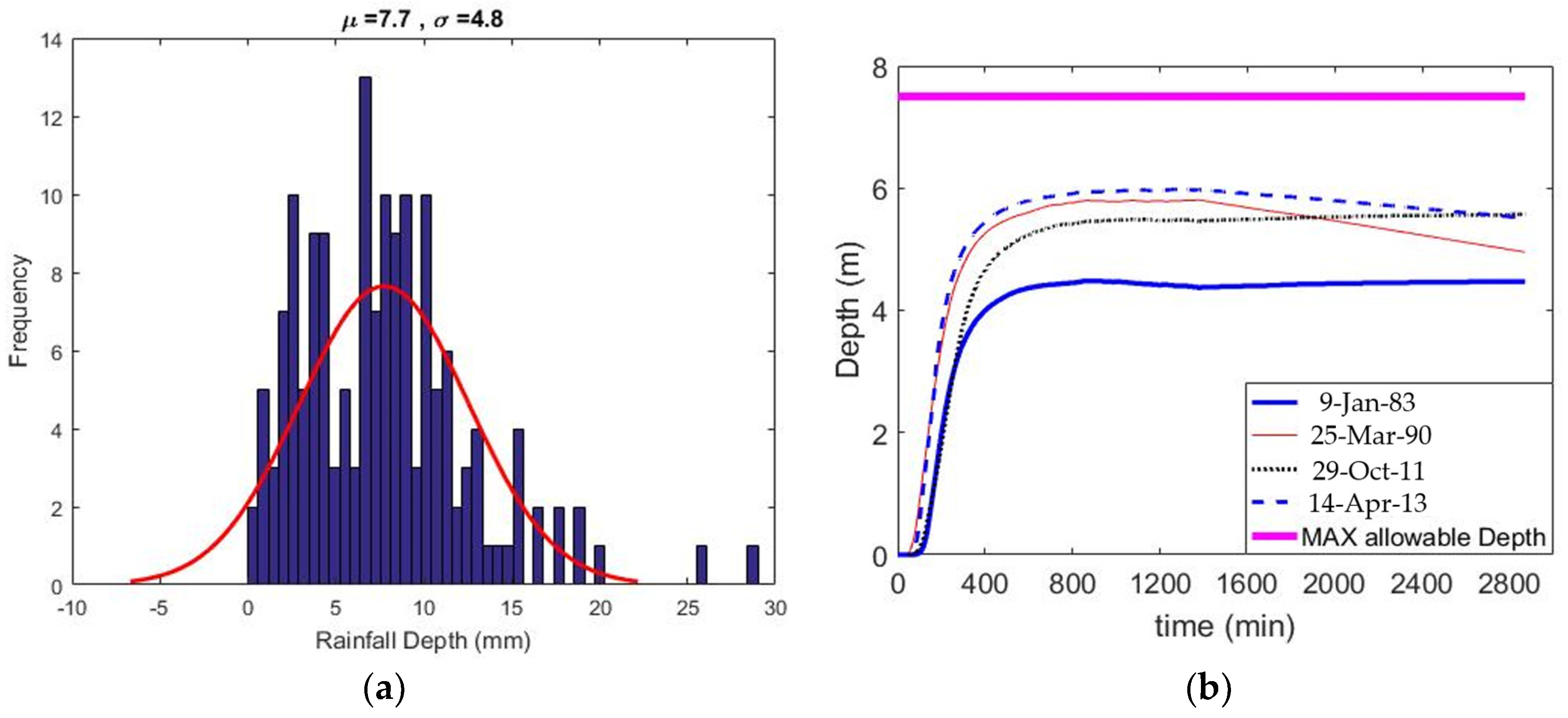
Figure 1. Flow diagram of the adaptive PR-MPC operation model.
Hydrology 10 00139 g001
Figure 2. Illustration of rainfall forecasting scheme having an input forecast time horizon (IFTH) and finer time-resolution predictors than input forecast time interval (IFTI).
Hydrology 10 00139 g002
Figure 3. Discrete water levels in the detention reservoir.
Hydrology 10 00139 g003
Figure 4. Map of Tehran Central Basin, the associated network modeled by SWMM, and Saleh-Abad reservoir intake structure [49].
Hydrology 10 00139 g004
Figure 5. Variation of the total available rainfall events in terms of depth and duration.
Hydrology 10 00139 g005
Figure 6. Structure of MLFNN model for the set of predictors and Sensitivity analysis made for determining the optimal number of neurons in the hidden layer.
Hydrology 10 00139 g006
Figure 7. Comparison of observed and forecasted rainfalls for test dataset resulted from scenario III’s set of predictors for different clusters (a) C1, (b) C2, (c) C3, and (d) C4.
Hydrology 10 00139 g007
Figure 8. (a) Histogram of the rainfall depth for the fourth cluster, C4 (b) Results of the reactive RTC model [24] in terms of variation of water level in the detention tank for four sample events of C4.
Hydrology 10 00139 g008
Figure 9. Comparison of flood hydrographs resulted from ideal Model A, the PR-MPC Model C, and the RE-MPC Model E for events 5 and 3.
Hydrology 10 00139 g009
Figure 10. Comparison of observed and predicted rainfall data obtained by the proposed short-term rainfall forecast model for two investigated events that occurred on 13 February 2002 and 30 January 2013.
Hydrology 10 00139 g010
Figure 11. The evolution of Model C’s solution features, i.e., flood volume, flood peak, and time to peak, over a subsequent sampling time interval ( T i compared with those of ideal Model A, for two investigated events occurred on 13 February 2002 and 30 January 2013).
Hydrology 10 00139 g011
Table 1. Investigated rainfall events.
Event No.EventDuration (min)Depth (mm)
19-Jan-8324014.35
225-Mar-9027020.29
313-Feb-0275026.41
429-Oct-1124016.9
530-Jan-1345024.1
614-Apr-1319518.8
Table 2. Clusters of the rainfall events found by the K-means algorithm.
Number of
Events Included
Included
Events (%)
Number
of Data
Average
Duration
(min)
Average
Depth (mm)
Max Depth
(mm/15 min)
All Data3351008063487.8413.510.59
C152162576951.921.26.3
C2105312915530.115.57.31
C318512951624.229.14.57
160481277181.47.710.59
Table 3. R2 values obtained by three ANN models, each for one of three sets of predictors (scenarios) for both training and test datasets and for different data clusters.
Scenario All DataC1C2C3C4
ITrain0.410.490.440.550.28
Test0.390.470.430.520.25
IITrain0.430.530.470.700.35
Test0.420.510.460.680.31
IIITrain0.470.610.570.750.42
Test0.450.590.550.730.42
Table 4. Different MPC-based models and their features in terms of the forecast type or accuracy (perfect and imperfect) and the forecast time horizon (IFTH).
ModelInput Forecast Type in Terms of IFACIFTH
APerfect (error-free)Entire rainfall event
BPerfect (error-free)Two time-steps ahead
CImperfect use forecasting moduleTwo time-steps ahead
DImperfect use forecasting moduleOne time-step ahead
EWithout a forecast module (reactive model)(reactive model)
Table 5. Comparison of performance of the five different MPC-based models in terms of flood volume inundation considering two rainfall events.
ModelEvent: 13 February 2002Event: 30 January 2013
Flood Reduction Compared with Model EFloodingFlood Reduction Compared with Model EFlooding
(103 m3)(103 m3)
(%)(103 m3) (%)(103 m3)
A10%38.9334.3725%17.1152.07
B4%12.87360.415%10.0859.1
C3%10.56362.7111%7.6561.53
D2%6.57366.72%1.367.88
----373.27----69.18
Disclaimer/Publisher’s Note: The statements, opinions and data contained in all publications are solely those of the individual author(s) and contributor(s) and not of MDPI and/or the editor(s). MDPI and/or the editor(s) disclaim responsibility for any injury to people or property resulting from any ideas, methods, instructions or products referred to in the content.

