Article

Quantitative Estimation of Rainfall from Remote Sensing Data Using Machine Learning Regression Models

1
Loboratoire d’Analyse et de Modélisation des Phénomènes Aléatoires, LAMPA, Faculté du Génie Electrique et d’Informatique (FGEI), University Mouloud MAMMERI of Tizi Ouzou (UMMTO), Tizi Ouzou 15000, Algeria
2
ECAM-EPMI, LR2E-Lab, Laboratoire Quartz, 95092 Cergy Pontoise, France
*
Author to whom correspondence should be addressed.
Hydrology 2023, 10(2), 52; https://doi.org/10.3390/hydrology10020052
Submission received: 24 December 2022 / Revised: 9 February 2023 / Accepted: 12 February 2023 / Published: 16 February 2023
(This article belongs to the Special Issue Recent Advances in Water and Water Resources Engineering)

Abstract

:
To estimate rainfall from remote sensing data, three machine learning-based regression models, K-Nearest Neighbors Regression (K-NNR), Support Vector Regression (SVR), and Random Forest Regression (RFR), were implemented using MSG (Meteosat Second Generation) satellite data. Daytime and nighttime data from a rain gauge are used for model training and validation. To optimize the results, the outputs of the three models are combined using the weighted average. The combination of the three models (hereafter called Com-RSK) markedly improved the predictions. Indeed, the MAE, MBE, RMSE and correlation coefficient went from 23.6 mm, 10.0 mm, 40.6 mm and 89% for the SVR to 20.7 mm, 5.5 mm, 37.4 mm, and 94% when the models were combined, respectively. The Com-RSK is also compared to a few methods using the classification in the estimation, such as the ECST Enhanced Convective Stratiform Technique (ECST), the MMultic technique, and the Convective/Stratiform Rain Area Delineation Technique (CS-RADT). The Com-RSK show superior performance compared to ECST, MMultic and CS-RADT methods.The Com-RSK is also compared to the two products of satellite estimates, namely CMORPH and CHIRPS. The results indicate that Com-RSK performs better than CMORPH and CHIRPS according to MBE, RMSE and CC (coefficient correlation). A comparison with three types of satellite precipitation estimation products, such as global product, regional product, and near real-time product, is performed. Overall, the methodology developed here shows almost the same results as regional product methods and exhibits better results than near real-time and global product methods.

1. Introduction

In Algeria, the climate tends to become dry. The amount of precipitation has dropped considerably, and measuring it using traditional means, such as ground radars and rain gauges, remains insufficient for superior quantification. Moreover, the availability of in situ data on large spatio-temporal scales is limited, and the required spatial domain coverage is small. There are additional disadvantages too, such as the difficulties of collection, the gaps in the recording of data and their subsequent interpolation, and the lack of digitization [1]. Thus, as an alternative solution, remote sensing data are used a great deal for the elaboration of precipitation maps [2,3,4,5,6,7]. They are available on large spatio-temporal scales and are collected continuously and regularly. This type of data covers large areas of the globe.
However, remote sensing data from geostationary weather satellites are not direct measurements of precipitation totals. They provide information on the temperature of cloud tops, on the optical and microphysical properties of clouds, and on the vertical development of clouds. To link this information to precipitation rates, certain methods are used [2,8,9,10]. Many of these method proceed by classifying remote sensing data into precipitation intensities [11,12,13]. Recently, methods based on machine learning using classification models have been implemented, such as an artificial neural network [14], a support vector machine [15], a random forest [5], K-Nearest Neighbors [16], naive Bayes [4], or combinations among these models [3,10,17,18]. In addition, for the estimation of precipitation, deep learning was used [19,20]. Indeed, deep learning based on deep neural networks shown its effectiveness in detection of images and in object recognition [21]. Deep learning as a convolution neural network (CNN) treats a set of pixels (an object) that permits detection and recognition of the object. In this treatment, convolution and pooling are repeated before being connected to an MLP (multilayer perceptron). The MLP generates the response (object detected) as output. With precipitation classification that is performed at the pixel scale, deep learning using a CNN cannot be applied. In the case of the DNN (deep neural network), the problem is the complexity and the volume of data required. In the context of this study, the quantity of data provided by the MSG (Meteosat Second Generation) is insufficient for the DNN implementation.
The results obtained showed the effectiveness of machine leaning, and the performances reached significant levels. However, classification has dominated the applications, and extremely few cases have used regression in precipitation estimates. However, machine learning (ML) can be used effectively in classification and regression; itcanconsider a large number of variables and complex interactions between variables.ML-based models are able to learn from the data, and thus predict the output [22]. The significant difference between classification and regression is that classification predicts a discrete class while regression helps predict a continuous quantity. Sometimes there are overlaps between the two mechanisms. For example, Castillo-Botón et al. [23] applied a set of machine learning classification and regression methods for fog events predictions. These methods showed that the unbalanced nature of the classification problem presents a difficulty for obtaining important results. On the other hand, regression methods have the advantage of not requiring any rebalancing to obtain accurate prediction results. Siirtola and Röning [24] made a comparison between classification models and regression models for User-Independent and Personal Stress Detection. According to the results found in this study, regression models outperform classification models. Shuze Guo et al. [25], however, show that the classification model is generally better than the model of the regression that they applied in an urban tourism competitiveness evaluation system. Yet, the general tendency points out that the choice between regression and classification lies above all in the type of variable to be predicted—continuous or discrete.
In the context of rainfall quantification, as indicated previously, in recent years we have witnessed a growing use of models based on machine learning in the classification and estimation of precipitation intensities based on instantaneous data from satellite remote sensing [17,26]. Target outputs represent interval classes. To estimate precipitation, a rain rate is assigned to each of the classes. The estimation of precipitation in this case will depend greatly on these classifications, and the results are not generally correlated with rainfall data, especially on short-term scales [27]. Additionally, in classification in general, the pairs of data are the instantaneous measurements of the meteorological radar and instantaneous satellite observations. Poorly calibrated radar affects classifications and ratings. As for the rain gauge data, the instantaneous measurement does not correspond to the immediate satellite observation. This time lag can also affect classifications and estimates.
To remedy this, for a direct estimation of precipitation rates, regression is usually recommended, especially since the estimation of precipitation gives quantitative predictions. In the literature, very rarelyare case studies conducted for the estimation of precipitation using regression [9]. With regression, the target output is a direct estimate of a rainfall amount. To reduce the time lag, the rain gauge data over daytime and nighttime periods are compared with the average of the satellite observations during the same period.
The objective of this paper is to estimate precipitation using regression models based on machine learning from MSG (Meteosat Second Generation) data. These are K-Nearest Neighbors regression (K-NNR), Support Vector Regression (SVR), and Random Forest Regression (RFR). MSG data and rain gauge data pairs are matched for learning and validating regression models. This attempts to link remote sensing data from space to rainfall totals.
The next sections of this study are organized as follows. In Section 2, the study region and the type of data used are described. The methodology developed for the estimation of precipitation is presented in Section 3. The applications of the models are presented in Section 4.The conclusion and perspectives are the subjects of Section 5.

2. Study area and Data

We applied the regression models to establish the relationship between MSG satellite data and rain gauge data. The study area covers the northern region of Algeria (See Figure 1).
It is located between latitudes 33° and 37°, longitudes −2° and 8°. This region has a Mediterranean climate. The rainy season runs from October to March, with maximum rainfall from November to December. The average annual rainfall is between 300 mm and 400 mm. Some areas record a minimum of about 60 mm, while the maximum is observed in the Djurdjura massif located in Kabylie and the Edough massif, where it exceeds 1500 mm.
In recent years, precipitation has become scarce and its estimation is essential for a better quantification in order to meet all hydrological and agricultural needs. However, with traditional means, this measurement remains incomplete. The Algerian National Meteorological Organization has a few rain gauges spread over the territory that provide occasional but reliable measurements. On the other hand, satellite observations from MSG are available on a regular basis.

2.1. Rain Gauge Data

The reference data used in this study come from the 146 rain gauges distributed over the study area. These rain gauges collect measurements on an hourly basis. We were therefore able to build a database composed of day and night accumulations throughout the study period. This day and/or night scale, represents the basis for learning the models and their validation. These data are collected during two rainy seasons (2008/2009 and 2009/2010).

2.2. MSG Data

The remote sensing data from space used to estimate precipitation come from an MSG (Meteosat Second Generation) geostationary meteorological satellite. This satellite observes the study area and provides data in the form of images in 12 channels from visible to infrared. The acquisition frequency is 15 min with a spatial resolution for the study area of 4 ×5 km2 (3 ×3 km2 at the sub-satellite point). Pixels coded on 10 bits are given in numerical count. The brightness temperatures “T” (Kelvin) for the infrared channels and the reflectance “Ref” for the visible channels [28] are calculated from the digital counts. This information is implicitly linked to rainfall rates.
In this study, in order to better exploit the range of frequencies from MSG, among the 12 channels in the visible (VIS), near infrared (NIR), and infrared (IR) domains [28,29], we have selected eight channels most closely related to precipitation, namely, VIS0.6, NIR 1.6, IR3.9, WV6.2, WV7.3, IR8.7, IR10.8 and IR12.0 (Table 1).
However, the visible channels (VIS0.6, NIR1.6) essential for obtaining information on the optical and microphysical properties of clouds are not available during nighttime. On the other hand, the IR3.9 channel, which is essential for characterizing precipitation, cannot be used during daytime because it is highly sensitive to solar radiation that disturbs infrared observations. Accordingly, we split the database into daytime data and nighttime data (see Table 1).
From these selected channels, we formed combinations to have information about the cloud optical and microphysical properties, the cloud top temperature, and the cloud vertical extension. The list of channels and combination of channels used as well as their availability are given in Table 1.

2.3. Coincidence MSG Data/ Rain Gauge Data

Spatial co-localization between MSG data and rain gauge data is determined using the conversion of GPS coordinates to pixel coordinates [29]. In addition, to have the maximum of spatial coincidences, the average of the 5 × 5 pixels centered above the rain gauge was used for all the channels and compared to the corresponding rain gauge.
As for temporal coincidences, for each rain gauge that recorded an accumulation during the daytime (respectively during the nighttime), we compared the average of the values observed by MSG during this same period.

3. Methodology

We implemented three regression models (SVR, RFR and K-NNR) based on machine learning for the direct estimation of precipitation from satellite observations. First, the different models are used separately, receiving at the input the spectral information from the MSG satellites, generating at the output a prediction based on the regression. The three individual predictions obtained are then combined using the weighted average. This combination is hereinafter called Com-RSK (combination of RFR, SVR and K-NNR). The plan of the methodology is given as follows:
  • Mathematical description of the models
  • Models learning and tuning
  • Combination of three models

3.1. Mathematical Description of the Models

3.1.1. Support Vector Regression

Support Vector Machine (SVM) is a widely used algorithm and is among the most reliable machine learning algorithms (Maroco et al., 2011). SVM can be used for classification problems or regression problems, which in this case can be called SVR (Support Vector Regression) with the incorporation of an ɛ-insensitive loss function [33]. In the latter case, the target is a continuous response. As for SVMs, in nonlinear cases, SVR employs kernels for better prediction [34]. The SVR minimizes an ɛ-insensitive loss function (see Equations (1) and (3)):
I ε = { 0 | y i f ( x i ) |
If | y i f ( x i ) | < ε , otherwise, for a linear function given by Equation (2):
f ( x ) = β 0 x i t β
where β is the coefficient calculated in regression, the loss function is:
i = 1 n max ( y i x i t β β 0 ε ,   0 )
where ε is the turning parameter and is expressed according the Equations (4) and (5)
minimize:
1 2 β 2
subject to:
{ y i x i t β β 0 ε , ( y i x i t β β 0 ) ε
In case all variables fall outside the error boundary, no solution is generated, hence slack variables, γI and γI* a are used to put the observations in the regression line (Equation (6))
{ y i x i t β β 0 ε + γ ( y i x i t β β 0 ) ε + γ i * γ i γ i * 0

3.1.2. Random Forest Regression

The random forest (RF) model based on machine learning performs classification and regression [35,36]. As with classification, the RF Regression model makes the decision from a set of regression trees called bagging. This algorithm operates as follows:
  • Creation of the first regression tree from a bootstrap sample taken at random from the database and then returned.
  • Creation of the other regression trees in the same way as the first step.
  • The final decision is the arithmetic mean of the regression results given by all the decision trees composing the random forest.
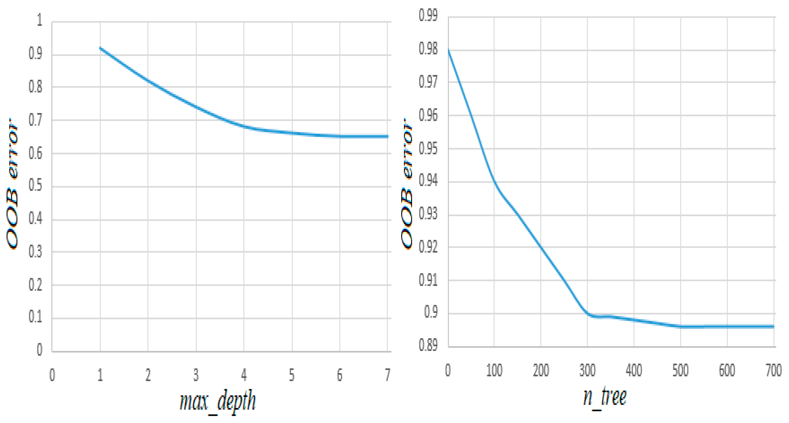
In the tuning, these are only two parameters to adjust for an optimal RFR, the number of trees in the forest (n_tree) and the number of variables in the random subset at each node (max_depth) [37]. These parameters are adjusted according to OOB (Out-of-Bag) Error which must be minimal. The OOB error represents the error between the predictions obtained by the model through the various trees on the data that have not been integrated into the learning and the real measurements.

3.1.3. K-Nearest Neighbor Regression

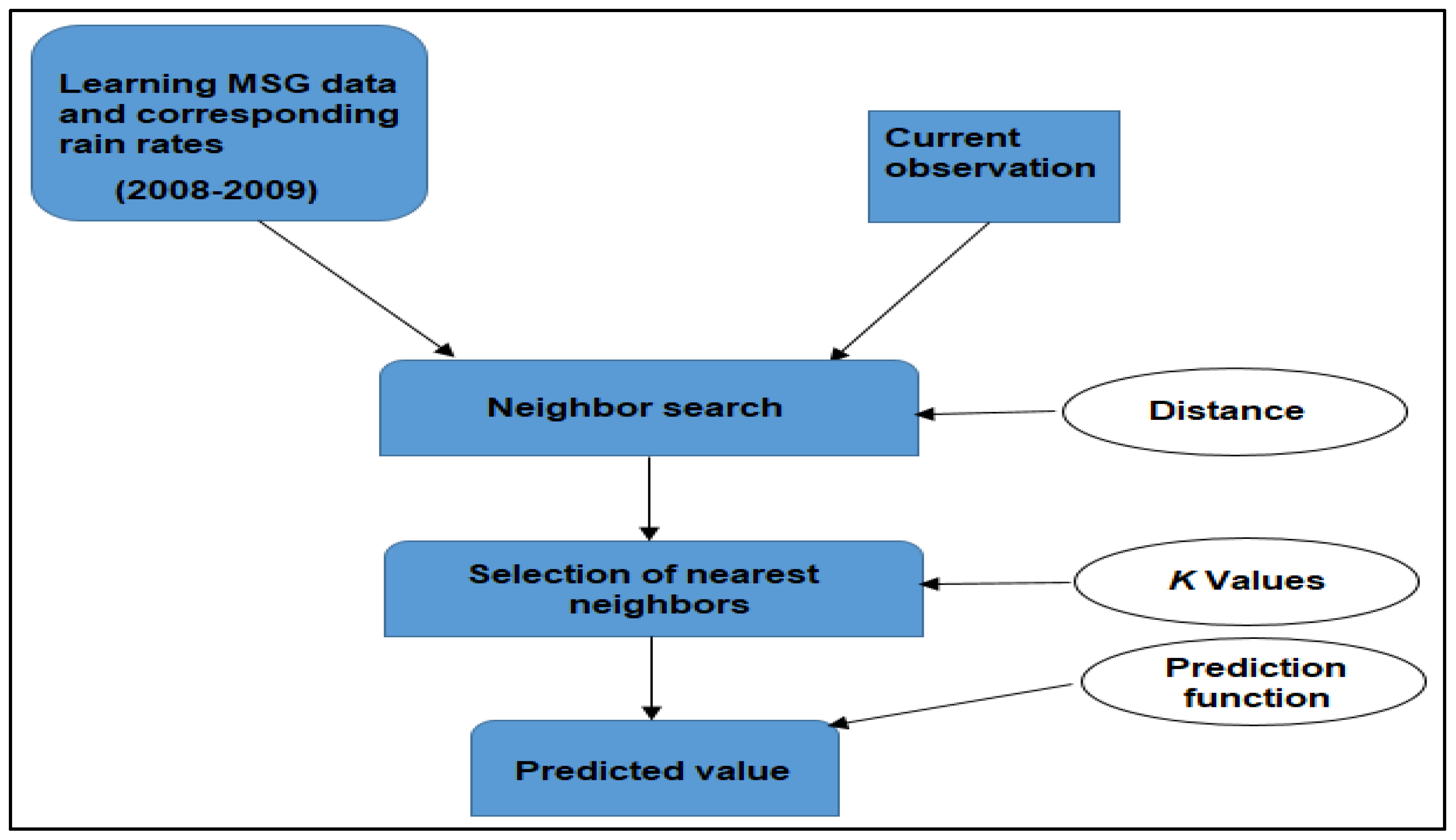
The KNN model was developed for classification [38]. In recent decades, the KNN has shown very interesting performances in nonparametric regression. The basic operation process of KNN model can be summarized as follows:
  • Construction of a learning database D composed of the inputs and the corresponding outputs.
For a new observation X whose output variable we want to predict, we proceed as follows:
  • Calculate all the distances between this observation X and the other observations of the data set D
  • Select the K observations closest to X according to the distance
  • Calculate the average of the K observations retained in the case of the regression.

3.2. Learning and Tuning Models

For the development of this regression, we compared the satellite spectral information to the rainfall measurements collected by the rain gauges. The learning and validation periods are given in Table 2.
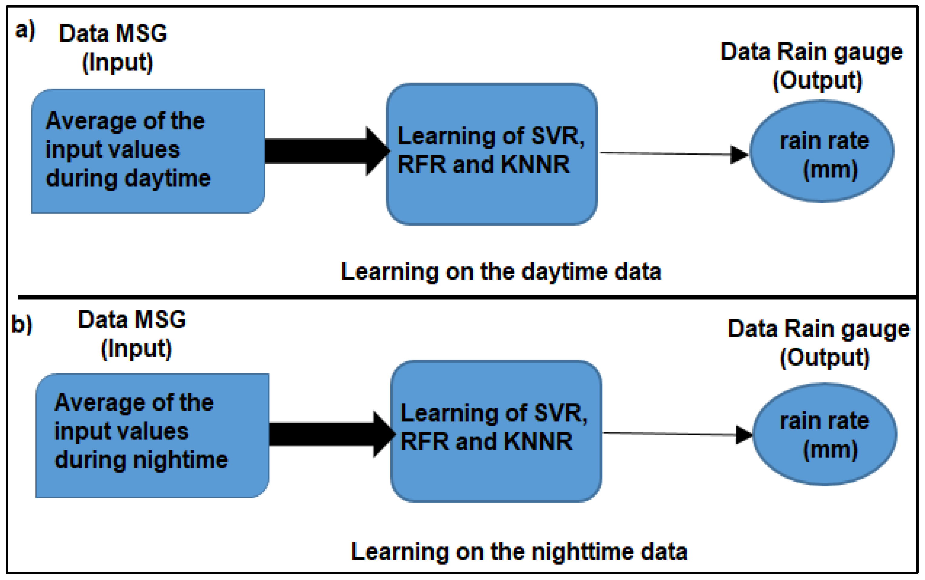
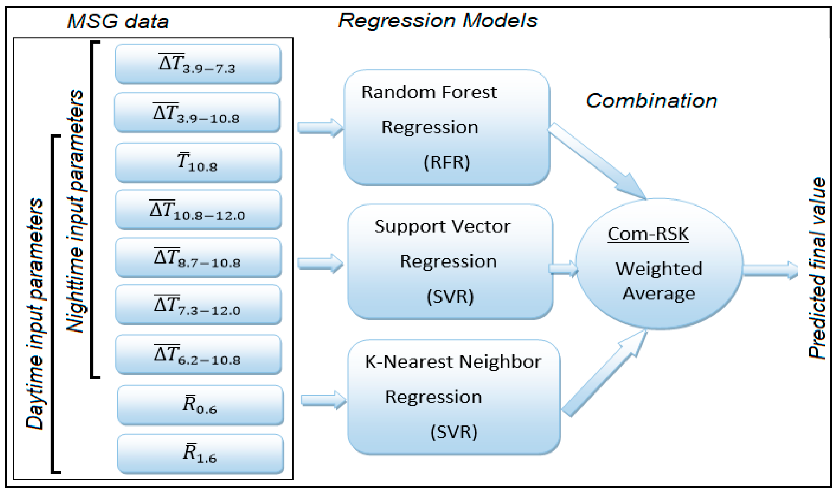
The acquisition of rain gauge measurements is obtained on an hourly time scale. To reduce the time lag error between satellite observations and the amount of rainfall on the ground on the one hand, and to exploit information on the optical and microphysical properties of clouds provided from the visible and infrared channels of MSG on the other hand, we designed two learning regressions. The first learning regression is performed between the daytime spectral information and the corresponding rain gauge measurements, while the second learning is performed between the nighttime spectral information and the corresponding rain gauge measurements (see Figure 2).
To do this, the averages of the instantaneous input information of each parameter and for each daytime and nighttime periods and the corresponding target output (raingauge measurements) are used.The average of each input parameter is calculated by using the Equation (7).
X ¯ p a r a ( i ) = t = 1 n X p a r a ( i ) ( t ) n
where X p a r a ( i ) ( t ) is the value (reflectance or brightness temperature) of parameter i(input parameters) at time t. The n is the number of observations taken during daytime (respectively night-time).

3.2.1. Tuning of RFR

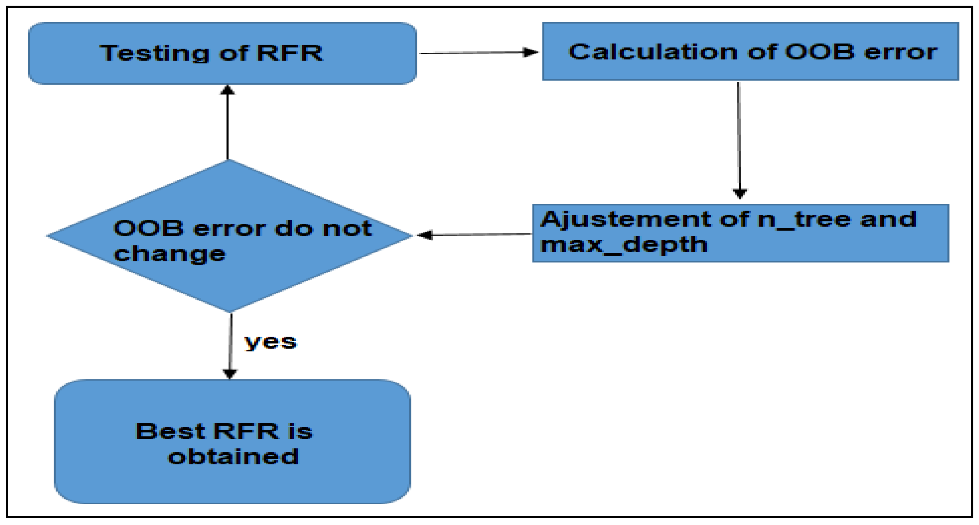
The optimization of the RFR (random forest regression) model consists in finding the optimal values for the number of decision trees (n_tree) and the maximum tree depth (max_depth). These values correspond to the smallest error of OOB. To do this, two-thirds of the training data is used in building the RFR.
The remaining third, called OOB data, is used for testing by calculating the deviations between the predicted value and the observed value represented by the OOB error (Equation (8)).
E O O B = 1 | p | i p ( h ( n _ t r e e i , max _ d e p t h i ) Y i ) 2
where p is the number of samples of OOB data, h ( n _ t r e e i , max _ d e p t h i ) is the prediction for sample i for n_tree and max_depth and Y the actual measurement. This operation permits selection of the optimal values for n_tree and max_depth. The optimization scheme of the n_tree and max_depth is given by Figure 3.
The results of these tests are shown in Figure 4 where we noted the best fit of RFR is obtained with n_tree = 500 and max_depth = 6.

3.2.2. Tuning ofK-NNR

In the case of K-NNR, we constructed the regression scheme shown in Figure 5. The final predictor function in this regression is the average obtained from the K nearest neighbors.
To select the best K-NNR, we performed the regression on the tuning data by testing two distances, namely the Euclidean distance (Equation (9)) and the Manhattan distance (Equation (10)) while varying the value of K (number nearest neighbours).
D e ( x , y ) = j = 1 n ( x i y j ) 2
D m ( x , y ) = j = 1 n | x j y j |
We used R-squared (R2) which is a statistical measure to select the best combinations (distance and value of k). The R-squared which is the squared correlation coefficient (CC) is calculated by Equation (11)
R - s q u a r e d = ( [ ( E i E ¯ ) ( M i M ¯ ) ] ( E i E ¯ ) 2 ( M i M ¯ ) 2 ) 2
where Ei and Mi are the ith estimation using the satellite method and measurement using rain gauge, respectively.
The result on the tuning data for the two distances by varying the numbers K is shown in Figure 6.
According to these results, the best K-NNR (R-squared = 0.85) is obtained for the Euclidean class with K = 10.

3.2.3. Tuning of SVR

For tuning of the SVR, we selected the best kernel function by performing tests. Support vectors correspond to observations outside of the error boundary. In our case, the data set has an obvious non-linearity. Therefore, in the regression used, the kernel function is incorporated to highlight the regression space suitable for this nonlinearity. Kernel functions facilitate assignment for nonlinear cases and speed up computation. These cores allow creation of a window to influence the data. We tested four kernel functions given by Equations (12)–(15).
Gaussian   Kernel   Exponential   ( GKE ) :   K ( x , y ) = e ( x y 2 2 σ 2 )
Gaussian   Kernel   Radial   Basis   ( GKRB ) :   K ( x , y ) = e ( γ x y 2 )
Sigmoid   kernel   ( SK ) :   K ( x , y ) = tan h ( γ x T y + r )
Polynomial   kernel   ( PK ) :   K ( x , y ) = tan h ( γ x T y + r ) d
The parameter r is a constant that can be used to control the trade-off between training data fit and margin size. Thus, the r-value, if large, gives low training error but results in overfitting. In contrast, a small value of r gives a high training error but results in underfitting.
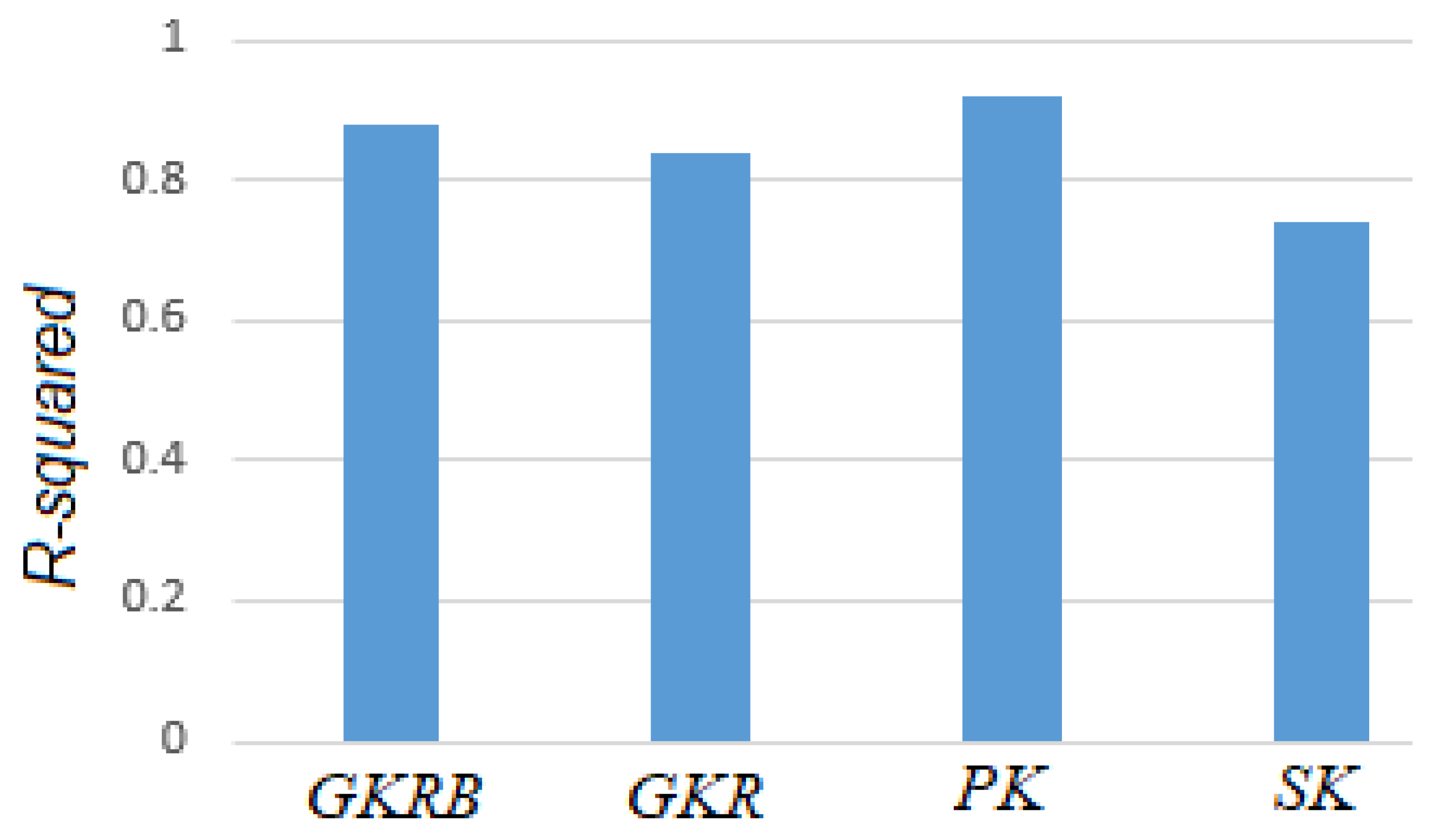
As for the K-NNR, we used R-squared (R2) to select the best kernel function. On the tuning data, we applied SVR using the different kernel functions. The R-squared values obtained for the different kernel functions are shown in Figure 7.
The results from Figure 7 show that the best SVR is obtained with the Polynomial kernel function with R-squared of 0.88.

3.2.4. Test of Input Parameters

After identifying the best RFR, SVR and K-NNR, we studied the sensitivity of the regression framework to various input parameters. This also allows selecting the best combination of input parameters. For each combination with 1, 2, 3, 4, 5, 6 or 7 input parameters, we calculated the R-squared. Table 3 illustrates the ranges of R-squared values.
The sensitivity of the regression framework to various input parameters was analyzed. According to the results obtained from Table 3, the best correlation is observed when the 7 input parameters are combined for the three regression models. Thus, for the rest, all results are determined using the combination of the seven input parameters.

3.3. Combination of Models

For improving the prediction results, we combined the three best variants of models after tuning (Com-RSK). Contrary to the classification which uses the majority vote, the most used combination in the regression is the average of the predictions. However, since the levels of performance of the models are different, we opted for the weighted average to achieve the combination. To do this, for each model, we calculated R-squared (R2), which is used as a weighting coefficient. R-squared (R2) can be used to evaluate the performance of a regression model by measuring the level of the correlation. Thus, the three predictions resulting respectively from the three regression models by considering the multispectral parameters MSG and R-squared (R2) of each model are determined. The final prediction is therefore calculated using the Equation (16):
P r e F i n a l = R S V R 2 × P r e S V R + R R F R 2 × P r e R F R + R K N N R 2 × P r e K N N R R S V R 2 + R R F R 2 + R K N N R 2
where P r e x is the prediction result given by model X (SVR, RFR or K-NNR).
The overall scheme of the methodology developed to integrate the combination is described in Figure 8. The model inputs correspond to the average of the k observations in each spectral parameter for the daytime period or for the nighttime period for which we compare the recorded accumulations by rain gauges at the same time.

4. Application for Rainfall Estimation

We applied the three regression models for the estimation of precipitation at daytime scale and nighttime scale as baseline estimation where the three models were trained. From these basic estimates, we also determined the estimates on a daily, monthly and seasonal scale by adding the basic estimates. In an attempt to improve the estimates, we combined the different models. The MSG input data and the corresponding reference data (rain gauge data) were collected during the 2009–2010 rainy season.
The different estimates were evaluated using the mean absolute error (MAE), mean bias error (MBE, or bias) and Root Mean Square Error (RMSE), calculated using the Equations (17), (18) and (19), respectively. The correlation between the regression estimates and the rain gauge measurements was also analyzed using the correlation coefficient CC.
M A E = 1 N i = 1 N | E i M i |
M B E = 1 N i = 1 N ( E i M i )
R M S E = 1 N i = 1 N ( E i M i ) 2
where Ei and Mi are the ith estimation using satellite method and measurement using rain gauge, respectively. The N is the number of coincidences between the estimates and measurements at the pixel scale.

4.1. Prediction Results

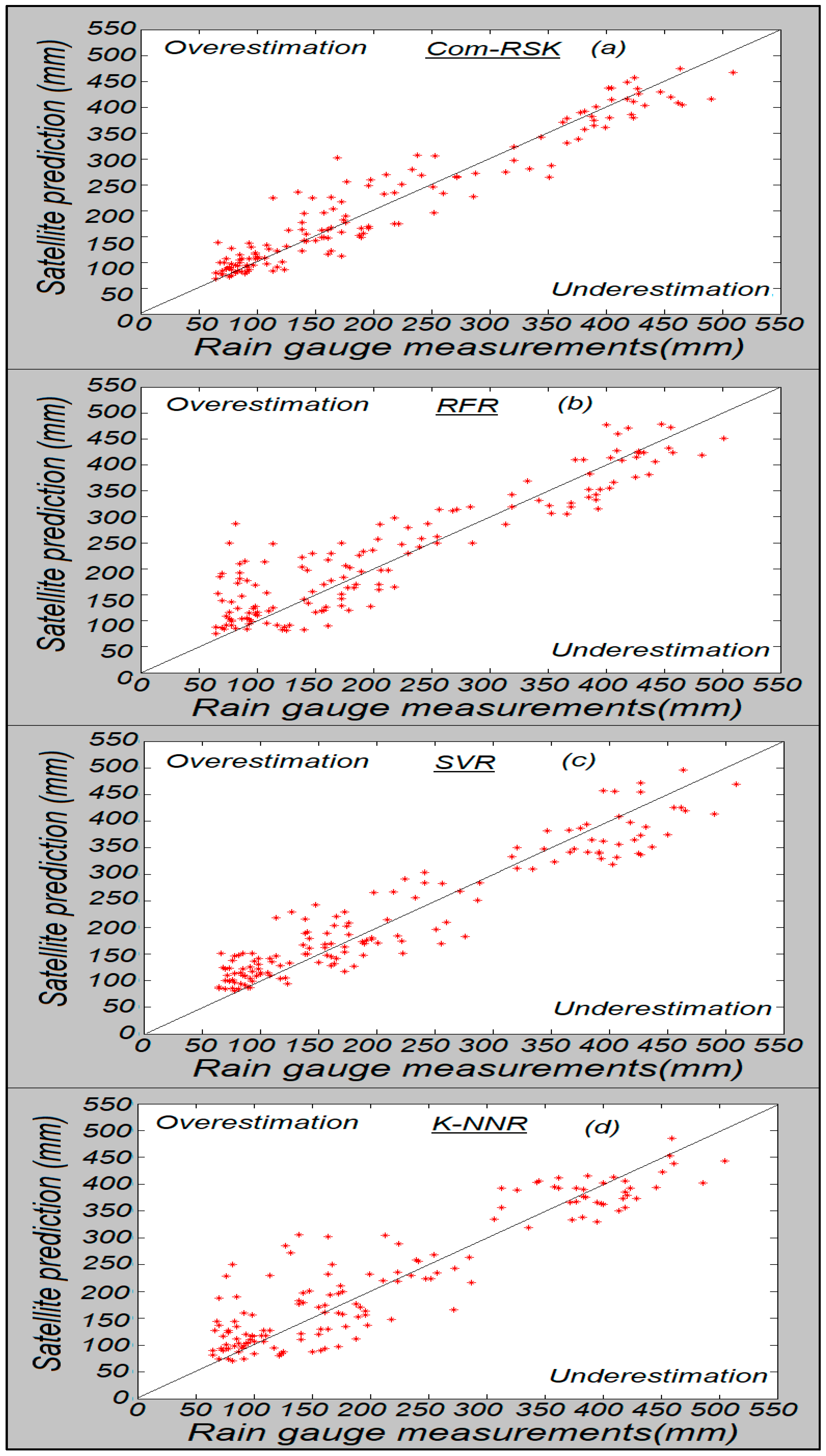
The results of the estimates obtained by the regression models confronted with the real measurements (rain gauge) on the various scales, namely, daily, monthly, and seasonally are given in Figure 9, Figure 10 and Figure 11, respectively. The corresponding statistical evaluation values for the three scales are also given in Table 4, Table 5 and Table 6, respectively. The average of the estimates for each model for each scale obtained was also calculated.
Figure 9 shows the estimates for 24 h (from 10 January 2010 at 7 a.m. to 11 January 2010 at 7 a.m.) of successive rains, performed by the different models against the actual measurements. It is a precipitation event composed mainly of stratiform rain. We also give the estimates obtained by the combination of the different models (Com-RSK).
Figure 10 illustrates the results of estimates versus rain gauge measurements for the month of January 2010 where stratiform and/or convective precipitation events occurred.
According to the Table 4, on a daily scale, the estimates, on the whole, are well correlated with the actual measurements. This correlation is more important for the SVR model where it reaches a value for the CC of 72% against 62% for K-NNR and 69% for RFR. In terms of MAE, MBE and RMSE for an average of 13.6 mm, the SVR shows better performance. Indeed, the values of MAE, MBE, and RMSE are 1.3 mm, 5.2 mm and 3.0 mm for SVR against 1.9 mm, 6.1 mm, and 3.6 mm for RFR and 2.5 mm, 6.7 mm, and 5.3 mm for K-NN, respectively. However, all models show an overestimation of precipitation. The combination of the three models by the weighted average significantly improved the results. The CC obtained returns to 78%, while MAE, MBE and RMSE indicate the values 1.0 mm, 4.1 mm and 2.1 mm, respectively.
The same trends with a slight improvement are observed for the monthly scale (see Table 5) and seasonal scale (see Table 6). Indeed, for the monthly scale, the SVR always shows superior performance compared to K-NNR and RFR. The CC indicates 85% for SVR against 72% for K-NNR and 74% for RFR. For an average of 75.9 mm, the SVR still shows the best values in terms of MAE, MBE and RMSE, 7.3 mm, 8.1 mm, and 14.1 mm for SVR and 8.2 mm, 9.2 mm, and 16.9 mm for RFR and 8.7 mm, 10.2 mm, and 17.3 mm for K-NNR. The overestimation was very slight contrary to the daily estimates presented above.
We also noted an improvement in these estimates when the models were combined. The MAE, MBE, RMSE, and CC parameters all showed better values compared to the individual use of the three models. As for the seasonal scale, the estimates are even better illustrated by the different values of MAE, MBE, RMSE, and CC. The combination shows very interesting performances compared to the separate use of the three models. A balance was obtained in terms of underestimation and overestimation. Stratiform type precipitation has been overestimated. The presence of convective precipitation gave a more balanced MBE.

4.2. Inter-Comparison

The elaborate regression method that combines three models was also compared to certain methods using classification in their estimates. They are:
  • The technique “Convective/Stratiform Rain Area Delimitation Technique (CS-RADT)” developed by Lazri et al. [8] uses the thresholds for the classification of precipitation into two types, convective and stratiform, from the spectral parameters of MSG. Then, a rainfall rate is assigned to each precipitation type for the precipitation estimate.
  • The ECST technique (Enhanced Convective stratiform technique) is elaborated by Reudenbach et al. [39] from the CST (Convective stratiform technique) originally presented by Adler and Negri [40]. The ECST is applied to extratropical regions and includes water vapor channels to separate cirrus from convective clouds [41].
  • The Multi-classifier model (MMultic), developed by Lazri et al. [17], is a technique based on machine learning. The technique combines Support Vector Machine (SVM), Artificial Neural Network (ANN), Weighted k-Nearest Neighbors (WkNN), Naive Bayes (NB), Random Forest (RF), and the Kmeans++ algorithm. The classification responses of the various models are then combined to generate a single optimized decision. To estimate, a rain rate is assigned to each precipitation type.
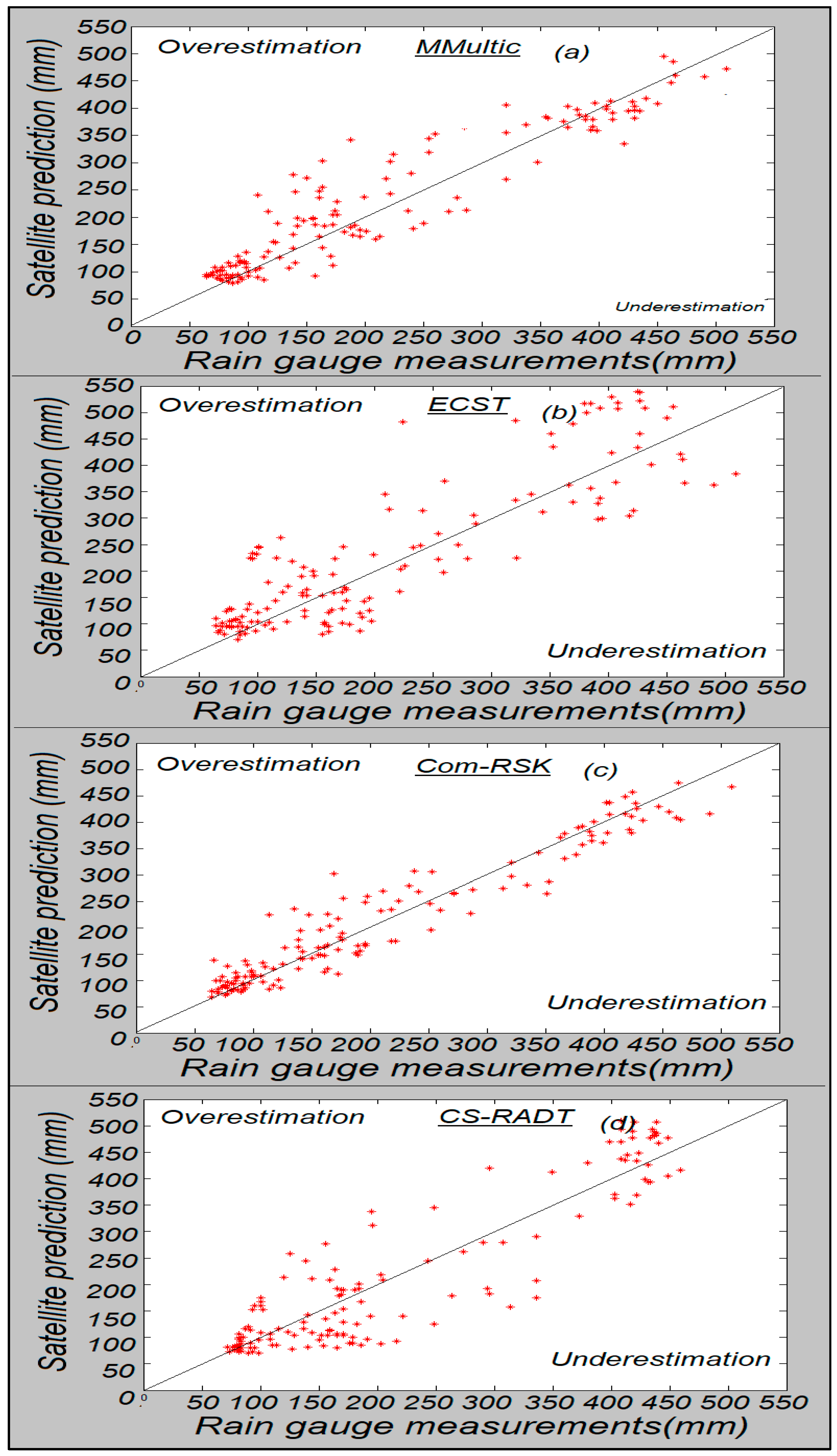
These methods operate in two steps for the estimation of precipitation:the classification of precipitation intensities and the determination of rain rates for each class. The results of the estimates on the seasonal scale by the different methods compared with the actual measurements are given in Figure 12.
The points of dispersion show that the fluctuations are highly important for the method based on the classification compared to the method of regression developed. Visually, the best correlation is observed for the Com-RSK, which combines the three regression models. Indeed, the CC is 94% for the Com-RSK against 93% for the MMultic method, 87% for the CS-RADT method and 81% for ECST (Table 7). The evaluation parameters MAE, MBE, and RMSE are also calculated (see Table 7).
According to Table 7, all values point to the performance of the Com-RSK. They thus confirm the superiority of the developed method of regression compared to the methods based on classification. For the developed regression method, in terms of MAE (mm), MBE, and RMSE (mm), we obtained 20.7 mm, 5.5 mm, and 27.4 mm versus 34.6 mm, 18.3 mm, and 52.9 mm for CS-RADT, 37.2 mm, 22.1 mm, and 55.8 mm for ECST, respectively. In the case of the MMultic method, we obtained 21.8 mm, 6.4 mm, and 41.6 mm, a performance that is lower than the developed regression method, despite the combination of six machine learning classifiers. This study showed the superiority of regression over classification in precipitation estimates. It is thus shown that it is preferable to use regression for the estimation of precipitation given the quantitative nature of the variable.
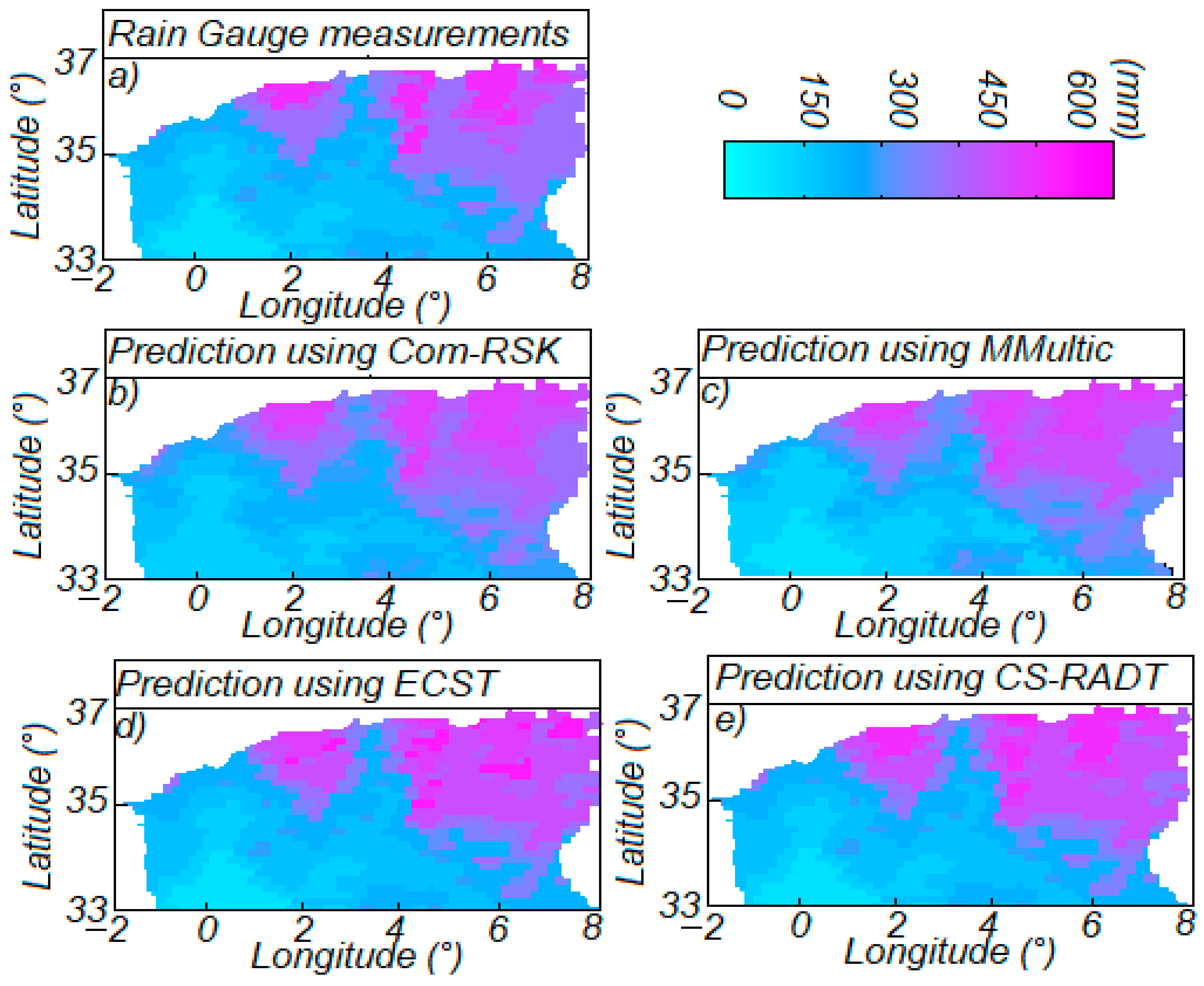
The spatial distribution of precipitation obtained by using Com-RSK over the North of Algeria is determined, based on an entire rainy season (Figure 13). The distributions performed by the methods MMultic, ECST and CS-RADT are also given. For a visual comparison, we gave the rain gauge measurements by carrying out extrapolations and interpolation.
The best correlation is observed for the estimates made by Com-RSK. The northeast part records more precipitation indicated by all the methods as well as by the rain gauge measurements. The south and northwest recorded low rainfall.
To better validate this study, we compared the developed method (Com-RSK) with two satellite methods, Climate Hazards Group InfraRed Precipitation with Stations (CHIRPS) and NOAA CPC Morphing Technique (CMORPH) applied to five regions in Algeria [42].The five regions overlap with our study area. The correlation coefficient (CC), MBE (mm), and the RMSE (mm) evaluation parameters are used to show the performance of the Com-RSK on the three scales, daily, monthly, and annual. In Table 7, the intervals (minimum value and maximum value) of the values of the parameters obtained by applying the two products CMORPH and CHIRPS for the five regions are presented. For comparison, the values of evaluation parameters on the different scales for the Com-RSK are also shown in Table 8.
The results presented are variable among the five regions with significant intervals. Errors appear to be higher in regions that have experienced significant precipitation rates. The Com-RSK shows interesting performances compared to the two satellite products, especially for the northern regions of Algeria. For the annual scale, a record overestimation (102.99 mm) is obtained in the case of the CMORPH product, while the CHIRPS product shows an overestimation of 56.48 mm against 5.5 mm for the Com-RSK. The minimum overestimation value obtained for the CHIRPS product is 6 mm which is less than 5.5 mm (Com-RSK). In the case of the RMSE error, the interval is between 59.29 mm and 264.66 mm for CMORPH and from 18.62 mm to 144.64 mm for CHIRPS against 37.4 mm for the developed method. The CC highlights a good correlation between the results of the developed method and rain gauge measurements compared to results from CMORPH and CHIRPS.
Almost the same pattern of results is observed for the daily and monthly scales. A single exception was noted in the case of the MBE for the monthly scale where the results are better for CMORPH and CHIRPS compared to the Com-RSK. In terms of correlation, the Com-RSK shows a notable superiority.
It should be noted that the few better results from CMORPH and CHIRPS are due to the fact that more southern regions which recorded low precipitation rates indicate low errors but cannot be considered for comparison with the Com-RSK because that is mainly applied to the northern region whose rainfall is high compared to the south.
In addition, a comparison with some global satellite precipitation estimation products was performed. This comparison shows the overall performance of the technique developed here compared to precipitation estimation products developed around the world. Therefore, the Com-RSK method is compared to a set of Satellite products described and applied by [43]. Three techniques were selected as Global products: the Satellite Mapping of Precipitation method (GSMaP), the Global Precipitation Climatology Project method (GPCP-1dd), and the Tropical Rainfall Measuring Mission method (TRMM-3B42).Three different satellite rainfall products, designed for applications over Africa or West Africa only, are considered to be regional products: the Estimation of Precipitation by SATellites–Second Generation method (EPSAT-SG), the Tropical Applications of Meteorology using the SATellite method (TAMSAT) and the Rain Fall Estimation method (RFE-2.0).Two near-real-time methods were selected: the Precipitation Estimation from Remotely Sensed Information using the Artificial Neural Networks method (PERSIANN) and the GPI method (Geostationary Operational Environmental Satellite (GOES) Precipitation Index).From the results presented by Jobard et al. [43], the regional products methods are superior in terms of performance compared to the near-real-time and Global products methods. The values of the statistical parameters for all these methods as well as for Com-RSK are given in Table 9.
According to the results presented in Table 8, the Com-RSK method presents correct performances compared to all the satellite products. The CC shows an extremely high level of correlation between the estimates and the rain gauge measurements for the Com-RSK method with 94%, while for the regional products, it fluctuates between 51% and 71%. For the near-real-time and Global products methods, the CC fluctuates between 49% and 58%, and between 46% and 60%, respectively.
In terms of the MBE, the Com-RSK method has the same characteristics as regional products. The Global products methods tend to underestimate precipitation, while near-real-time methods show a significant overestimation. In the case of the RMSE error, the Com-RSK shows the same results as the Global products methods and presents better results than near-real-time methods, but it is exceeded by the regional products methods.

4.3. Discussion

The study presented in this article focuses on a beneficial approach to rainfall estimation through the use of remote sensing data capable of providing complete and continuous coverage in space and time. For the African continent, the need for rainfall estimation has increased in recent years due to climate change. However, the deployment of traditional means of measuring precipitation in this part of the world is insufficient, while that measurement is considered useful [44,45,46]. In this context, the methodology developed makes it possible to estimate rainfall by exploiting the good spatio-temporal resolution of MSG geostationary satellite data. Regression using machine learning-based models gave direct estimates of rainfall. Contrary to the traditional means used for measuring precipitation, this study generates maps of precipitation over a vast region covered by geostationary satellites. The extrapolation of this regression to other regions can be planned. Regions in Africa with the same climatic conditions as those from this study can directly benefit from the model for rainfall estimation, such as regions in northern Africa with a Mediterranean climate where climatic conditions are identical.
However, the uncertainties in current research come from the lack of sufficient ground data for better calibration. Indeed, the few rain gauges used are sparse and can affect estimates.

5. Conclusions

Rainfall in the northern region of Algeria was estimated using regression from satellite remote sensing data. Three regression models based on machine learning, such as KNNR, SVR, and RFR, were applied. The learning and validation database is composed of pairs of MSG data/rain gauge data and daytime/ nighttime scales. Thus, estimates on time scales, such as daily, monthly, and seasonally were made using the three regression models. Overall, the results obtained are remarkably interesting. Indeed, the estimates are well correlated with the actual measurements from the rain gauges. The best predictions are obtained by applying the SVR model. Indeed, the SVR outperformed all models showing the lowest errors in terms of MAE, MBE and RMSE. As for the correlation coefficient, the SVR showed the highest correlation.
In an attempt to improve the predictions, we combined the three models into a single output using the weighted average. In all the tests and for the different scales, we noted a clear improvement compared to the separate use of the three models. The correlation is more important for Com-RSK with a correlation coefficient of 94%. We also obtained the lowest values of MAE, MBE, and RMSE, which are 20.7 mm, 5.5 mm, and 37.4 mm, respectively. The Com-RSK was also compared to some machine learning-based precipitation estimation techniques using classification. We conclude, within the framework of this study, that the regression makes it possible to better estimate the precipitation. The regression prediction results obtained outperform all results where classification is applied for estimation. Regression gives direct estimates of precipitation amounts, while classification selects intervals of precipitation intensities. In the same context, Com-RSK is compared to the two products of satellite estimates (CMORPH and CHIRPS) applied in the same study area. The Com-RSK has shown the best results in terms of MBE, RMSE, and CC. To obtain a global vision with the method developed in this study, a comparison among three types of precipitation estimation products, such as global product, regional product, and near real time product was performed. On the whole, the Com-RSK shows almost the same results as the regional products methods and presents better results than the near-real-time methods orthe global products methods.
It should be noted that the methodology developed in this study can be applied at any time of the year in this study region or other regions with the same climate. For a region with a different climate, the learning parameters must be updated to be adapted to the new climate configuration. The choice of regression models based on machine learning must be made objectively. Consequently, from our perspective on this study, it is interesting to develop a strategy to select the quality and number of the most suitable regression models for improvement in the estimation of precipitation.

Author Contributions

Conceptualization, Y.M. and M.L.; methodology, Y.M. and M.L.; software, F.O.; validation, M.L., Y.M. and S.A.; formal analysis, K.L.; investigation, R.A.; resources, K.L. and R.A.; data curation, M.L.; writing—original draft preparation, M.L.; writing—review and editing, Y.M.; visualization, K.L.; supervision, R.A.; project administration, S.A.; All authors have read and agreed to the published version of the manuscript.

Funding

This research received no external funding.

Data Availability Statement

Not appliable.

Conflicts of Interest

The authors declare no conflict of interest.

References

  1. Kinouchi, T. Synergetic application of GRACE gravity data, global hydrological model, and in-situ observations to quantify water storage dynamics over Peninsular India during 2002–2017. J. Hydrol. 2021, 596, 126069. [Google Scholar]
  2. Levizzani, V. Satellite rainfall estimations: New perspectives for meteorology and climate from the EURAINSAT project. Ann. Geophys. 2003, 46, 363–372. [Google Scholar]
  3. Tebbi, M.A.; Haddad, B. Artificial intelligence systems for rainy areas detection and convective cells’ delineation for the south shore of Mediterranean Sea during day and night time using MSG satellite images. Atmos. Res. 2016, 178, 380–392. [Google Scholar] [CrossRef]
  4. Hameg, S.; Lazri, M.; Ameur, S. Using naïve Bayes classifer for classification of convective rainfall intensities based on spectral characteristics retrieved from SEVIRI. J. Earth Syst. Sci. 2016, 125, 945–955. [Google Scholar] [CrossRef] [Green Version]
  5. Kuhnlein, M.; Appelhans, T.; Thies, B.; Nauss, T. Improving the accuracy of rainfall rates from optical satellite sensors with machine learning—A random forests- based approach applied to MSG SEVIRI. Remote Sens. Environ. 2014, 141, 129–143. [Google Scholar] [CrossRef] [Green Version]
  6. Goshime, D.W.; Absi, R.; Ledésert, B. Evaluation and Bias Correction of CHIRP Rainfall Estimate for Rainfall- Run off Simulation over Lake Ziway Watershed, Ethiopia. Hydrology 2019, 6, 68. [Google Scholar] [CrossRef] [Green Version]
  7. Goshime, D.W.; Absi, R.; Haile, A.T.; Ledésert, B.; Rientjes, T. Bias-Corrected CHIRP Satellite Rainfall for Water Level Simulation, Lake Ziway, Ethiopia. J. Hydrol. Eng. 2020, 25, 05020024. [Google Scholar] [CrossRef]
  8. Lazri, M.; Ameur, S.; Brucker, J.M.; Testud, J.; Hamadache, B.; Hameg, S.; Ouallouche, F.; Mohia, Y. Identification of raining clouds using a method based on optical and microphysical cloud properties from Meteosat second generation daytime and nighttime data. Appl. Water Sci. 2013, 3, 1–11. [Google Scholar] [CrossRef]
  9. Ouallouche, F.; Lazri, M.; Ameur, S. Improvement of rainfall estimation from MSG data using Random Forests classification and regression. Atmos. Res. 2018, 211, 62–72. [Google Scholar] [CrossRef]
  10. Sehad, M.; Ameur, S. A multilayer perceptron and multiclass support vector machine based high accuracy technique for daily rainfall estimation from MSG SEVIRI data. Adv. Space Res. 2020, 65, 1250–1262. [Google Scholar] [CrossRef]
  11. Feidas, H.; Giannakos, A. Classifying convective and stratiform rain using multispectral infrared Meteosat Second Generation satellite data. Theor. Appl. Climatol. 2011, 108, 613–630. [Google Scholar] [CrossRef]
  12. Nauss, T.; Kokhanovsky, A.A. Discriminating raining from non- raining clouds at mid latitudes using multispectral satellite data. Atmos. Chem. Phys. 2006, 6, 5031–5036. [Google Scholar]
  13. Thies, B.; Turek, A.; Nauss, T.; Bendix, B. Wather type dependent quality assessment of a satellite- based rainfall detection scheme for the mid-latitudes. Meteorol. Atmos. Phys. 2010, 107, 81–89. [Google Scholar] [CrossRef]
  14. Mohia, Y.; Ameur, S.; Lazri, M.; Brucker, J.M. Combination of spectral and textural features in the MSG satellite remote sensing images for classifying rainy area into Different classes. J. Indian Soc. Remote Sens. 2017, 45, 759–771. [Google Scholar] [CrossRef]
  15. Sehad, M.; Lazri, M.; Ameur, S. Novel SVM-based technique to improve rainfall estimation over the Mediterranean region (north of Algeria) using the multispectral MSG SEVIRI imagery. Adv. Space Res. 2017, 59, 1381–1394. [Google Scholar] [CrossRef]
  16. Bensafi, N.; Lazri, M.; Ameur, S. Novel WkNN-based technique to improve instantaneous rainfall estimation over the north of Algeria using the multispectral MSG SEVIRI imagery. J. Atmos. Sol. Terr. Phys. 2019, 183, 110–119. [Google Scholar] [CrossRef]
  17. Lazri, M.; Labadi, K.; Brucker, J.M.; Ameur, S. Improving satellite rainfall estimation from MSG data in Northern Algeria by using a multi-classifier model based on machine learning. J. Hydrol. 2020, 584, 124705. [Google Scholar] [CrossRef]
  18. Belmahdi, F.; Lazri, M.; Ouallouche, F.; Labadi, K.; Absi, R.; Ameur, S. Application of Dempster Shafer theory for optimization of precipitation classification and estimation results from remote sensing data using machine learning. Remote Sens. Appl. Soc. Environ. 2023, 29, 100906. [Google Scholar] [CrossRef]
  19. Oukali, S.; Lazri, M.; Labadi, K.; Brucker, J.M.; Ameur, S. Development of a hybrid classification technique based on deep learning applied to MSG/SEVIRI multispectral data. J. Atmos. Sol. Terr. Phys. 2019, 193, 105062. [Google Scholar] [CrossRef]
  20. Xue, M.; Hang, R.; Liu, Q.; Yuan, X.T.; L u, X. CNN-based near real time precipitation estimation from Fengyun- 2 satellite over Xinjiang, China. Atmos. Res. 2021, 250, 105337. [Google Scholar] [CrossRef]
  21. Kavitha, M.; Gayathri, R.; Polat, K.; Alhudhaif, A.; Alenezi, F. Performance evaluation of deep e-CNN with integrated spatial spectral features in hyperspectral image classification. Measurement 2022, 191, 110760. [Google Scholar] [CrossRef]
  22. Samuel, A.L. Some Studies in Machine Learning Using the Game of Checkers. IBM J. Res. Dev. 1959, 3, 210–229. [Google Scholar] [CrossRef]
  23. Castillo Botón, C.; Casillas Pérez, D.; Casanova- Mateo, C.; Ghimire, S.; Cerro- Prada, E.; Gutierrez, P.A.; Deo, R.C.; Salcedo Sanz, S. Machine learning regression and classification methods for fog events prediction. Atmos. Res. 2022, 272, 106157. [Google Scholar] [CrossRef]
  24. Siirtola, P.; Röning, J. Comparison of Regression and Classification Models for User independent and Personal Stress Detection. Sensors 2020, 20, 4402. [Google Scholar] [CrossRef]
  25. Guo, S.; Jiang, Y.; Long, W. Urban tourism competitiveness evaluation system and its application: Comparison and analysis of regression and classification methods. Procedia Comput. Sci. 2019, 162, 429–437. [Google Scholar] [CrossRef]
  26. Ouallouche, F.; Labadi, K.; Mohia, Y.; Lazri, M.; Ameur, S. Artificial Intelligence for Satellite Image Processing: Application to Rainfall Estimation. In Intelligent Systems and Application; Springer: Singapore, 2023; Lecture Notes in Electrical Engineering; Chapter 14; Volume 959, ISBN 978-981-19-6580-7. [Google Scholar]
  27. Belghit, A.; Lazri, M.; Ouallouche, F.; Labadi, K.; Ameur, S. Optimization of One versus All-SVM using Ada Boost algorithm for rainfall classification and estimation from multispectral MSG data. Adv. Space Res. 2023, 71, 946–963. [Google Scholar] [CrossRef]
  28. EUMETSAT. Applications of Meteosat Second Generation Conversion from Counts to Radiances and from Radiances to Brightness Temperatures and Reflectance. 2004. Available online: http://oiswww.eumetsat.org/WEBOPS/msginterpretation/inex.html (accessed on 20 December 2022).
  29. EUMETSAT. MSG Level 1.5 Image Data Format Description. Available online: http://www.eumetsat.int/website:home/Data/Products/Formats/index.html (accessed on 20 December 2022).
  30. Thies, B.; Nauss, T.; Bendix, J. Delineation of raining from non-raining clouds during night time using Meteosat-8 data. Meteorol. Appl. 2008, 15, 219–230. [Google Scholar] [CrossRef]
  31. Roebeling, R.A.; Feijt, A.J.; Stammes, P. Cloud property retrievals for climate monitoring: Implications of differences between SEVIRI on METEOSAT-8 and AVHRR on NOAA-17. J. Geophys. Res. 2006, 11, D20210. [Google Scholar] [CrossRef]
  32. Lazri, M.; Ouallouche, F.; Ameur, S.; Brucker, J.M.; Mohia, Y. Identifying Convective and Stratiform Rain by Confronting SEVERI Sensor Multispectral Infrared to Radar Sensor Data Using Neural Network. Sens. Transducers 2012, 145, 19–32. [Google Scholar]
  33. Vapnik, V. The Nature of Statistical Learning Theory; Springer: New York, NY, USA, 1995. [Google Scholar]
  34. Guenther, N.; Schonlau, M. Support vector machines. Stata J. 2016, 16, 917. [Google Scholar] [CrossRef] [Green Version]
  35. Breiman, L. Random forests. Mach. Learn. 2001, 45, 5–32. [Google Scholar] [CrossRef] [Green Version]
  36. Puissant, A.; Rougier, S.; Stumpf, A. Object-oriented mapping of urban trees using Random Forest classifiers. Int. J. Appl. Earth Obs. Geoinf. 2014, 26, 235–245. [Google Scholar] [CrossRef]
  37. Liaw, A.; Wiener, M. Classification and Regression by random Forest. R News 2002, 2, 18–22. [Google Scholar]
  38. Cover, T.; Hart, P. Nearest neighbor pattern classification. IEEE Trans. Inf. Theory 1967, 13, 21–27. [Google Scholar] [CrossRef] [Green Version]
  39. Reudenbach, C.; Heinemann, G.; Heuel, E.; Bendix, J.; Winiger, M. Investigation of summertime convective rainfall in Western Europe based on a synergy of remote sensing data and numerical models. Meteorol. Atmos. Phys. 2001, 76, 23–41. [Google Scholar]
  40. Adler, R.F.; Negri, A.J. A satellite infrared technique to estimate tropical convective and stratiform rainfall. J. Appl. Meteorol. 1988, 27, 30–51. [Google Scholar] [CrossRef]
  41. Tjemkes, S.A.; Van de berg, L.; Schmetz, J. Warm water vapour pixels over high clouds as observed by Meteosat. Contrib. Atmos. Phys. 1997, 70, 15–21. [Google Scholar]
  42. Babaousmail, H.; Hou, R.; Ayugi, B.; Tchalim Gnitou, G. Evaluation of satellite-based precipitation estimates over Algeria during 1998–2016. J. Atmos. Sol. Terr. Phys. 2019, 195, 105139. [Google Scholar] [CrossRef]
  43. Jobard, I.; Chopin, F.; Berges, J.C.; Roca, R. An inter comparison of 10-day satellite precipitation products during West African monsoon Int. J. Remote Sens. 2011, 32, 2353–2376. [Google Scholar] [CrossRef]
  44. Goshime, D.W.; Absi, R.; Ledésert, B.; Dufour, F.; Haile, A.T. Impact of water abstraction on the water level of Lake Ziway, Ethiopia. WIT Trans. Ecol. Environ. 2019, 239, 67–78. [Google Scholar] [CrossRef] [Green Version]
  45. Goshime, D.W.; Haile, A.T.; Absi, R.; Ledésert, B. Impact of water resource development plan on water abstraction and water balance of Lake Ziway, Ethiopia. Sustain. Water Resour. Manag. 2021, 7, 36. [Google Scholar] [CrossRef]
  46. Goshime, D.W.; Haile, A.T.; Rientjes, T.; Absi, R.; Ledésert, B.; Siegfried, T. Implications of water abstraction on the interconnected Central Rift Valley Lakes sub-basin of Ethiopia using WEAP. J. Hydrol. Reg. Stud. 2021, 38, 100969. [Google Scholar] [CrossRef]
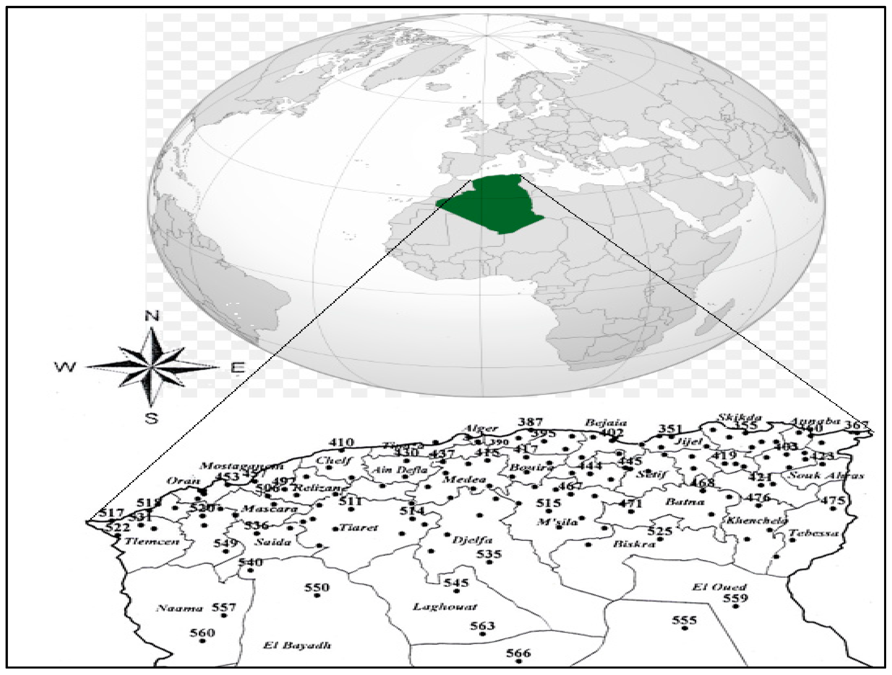
Figure 1. Study area and distribution of rain gauges in Northern Algeria.
Hydrology 10 00052 g001
Figure 2. Model training scheme, (a) for the daytime and (b) for the nighttime.
Hydrology 10 00052 g002
Figure 3. Flowchart for calculation of optimal values of n_tree and max_depth.
Hydrology 10 00052 g003
Figure 4. OOB error as a function of on max_depth and n_tree.
Hydrology 10 00052 g004
Figure 5. Flowchart of K-NN.
Hydrology 10 00052 g005
Figure 6. R-squared as a function of number of nearest neighbors applying Euclidean distance and Manhattan distance.
Hydrology 10 00052 g006
Figure 7. Value of R-squared using SVR for different kernel functions.
Hydrology 10 00052 g007
Figure 8. Overall regression scheme with combination step.
Hydrology 10 00052 g008
Figure 9. Satellite prediction vs .rain gauge measurements for the daily period, (a) using Com-RSK, (b) using RFR, (c) using SVR and (d) using K-NNR.
Hydrology 10 00052 g009
Figure 10. Satelliteprediction vs. rain gauge measurements for the monthly period, (a) using Com-RSK, (b) using RFR, (c) using SVR and (d) using K-NNR.
Hydrology 10 00052 g010
Figure 11. Satellite prediction vs. rain gauge measurements for the seasonal period, (a) using Com-RSK, (b) using RFR, (c) using SVR and (d) using K-NNR.
Hydrology 10 00052 g011
Figure 12. Satellite prediction versus rain gauge measurements for a seasonal estimation scale (a) using MMulti, (b) using ECST, (c) using Com-RSK and (d) using CS-RADT.
Hydrology 10 00052 g012
Figure 13. Spatial distribution of precipitation, (a) using rain gauge, (b) using Com-RSK, (c) using MMultic, (d) using ECST and (e) using CS-RADT.
Hydrology 10 00052 g013
Table 1. Channels and channels combinations with corresponding Range of values.
Channels and Channels Combinations
(Kelvin or µm)
DescriptionRange of ValuesClouds Characteristics
DaytimeNighttime
Τ10.8 (K)Brightness temperature in IR10.8207.2 k to 283.9 k205.3 k to 282.4 kVertical cloud extent and cloud top temperature [11,30].
ΔΤ10.8–12.0 (K)Brightness temperature difference between IR10.8 and IR12.0−0.3 k to 7.4 k−0.3 k to 7.1 kExistence of ice particles in the clouds [30].
ΔT8.7–10.8 (K)Brightness temperature difference between IR8.7 and IR10.8−4.6 k to 1.3 k−4.8 k to 1.7 kExistence of ice particles in clouds [31].
ΔT7.3–12.0 (K)Brightness temperature difference between IR7.3 and IR12.0−50.3 k to 6.6 k−52.0 k to 5.7 kCloud top temperature and Vertical cloud extension [11,32].
ΔT6.2–10.8 (K)Brightness temperature difference between IR6.2 and IR10.8−50.1 k to 6.4 k−51.8 k to 5.1 kVertical cloud extension, cloud top temperature [2,11].
R0.6 (µm)Reflectance in VIS0.60.02 µm to 1 µmNo usedCloud Particle Size and Cloud Optical Thickness [5,30].
R1.6 (µm)Reflectance in NIR1.60.03 µm to 1 µmNo usedCloud Particle Size and Cloud Optical Thickness [5,30].
ΔT3.9–7.3 (K)Brightness temperature difference between IR3.9 and IR7.3No used−4.9 k to 25 kCloud Particle Size and Cloud Optical Thickness [5,30].
ΔT3.9–10.8 (K)Brightness temperature difference between IR3.9 and IR10.8No used−10.3 k to 15.1 kCloud Particle Size and Cloud Optical Thickness [5,30].
Table 2. Periods of Learning, tuning and validation.
Rainy Season 2008/2009Rainy Season 2009/2010
SVRLearning (70%) and tuning (30%)Validation
RFRLearning (70%) and tuning (30%)Validation
K-NNRLearning (70%) and tuning (30%)Validation
Table 3. R-squared for the different combination using SVR, RFR or K-NNR.
CombinedInput ParametersNumber of CombinationsSVR
R-Squared
RFR
R-Squared
K-NNR
R-Squared
170.13 to 0.350.12 to 0.330.10 to 0.31
2210.17 to 0.380.14 to 0.380.14 to 0.35
3350.26 to 0.430.23 to 0.420.20 to 0.40
4350.34 to 0.560.33 to 0.520.34 to 0.52
5210.48 to 0.690.47 to 0.700.47 to 0.67
670.64 to 0.740.63 to 0.730.60 to 0.70
710.880.860.85
Table 4. Statistical parameters for the evaluation of the daily estimate.
Mean (mm)MAE (mm)MBE (mm)RMSE (mm)CC
SVR18.81.35.23.00.72
K-NNR20.32.56.75.30.62
RFR19.71.96.13.60.69
Com-RSK17.71.04.12.10.78
Optimal13.60001
Table 5. Statistical parameters for the evaluation of the monthly estimate.
Mean (mm)MAE (mm)MBE (mm)RMSE (mm)CC
SVR84.07.38.114.10.85
K-NNR86.18.710.217.30.72
RFR85.18.29.216.90.74
Com-RSK82.56.16.610.80.88
Optimal75.90001
Table 6. Statistical parameters for evaluating accumulation estimates for the entire rainy season.
Mean (mm)MAE (mm)MBE (mm)RMSE (mm)CC
SVR242.923.610.040.60.89
K-NNR249.228.316.343.50.87
RFR247.126.114.241.60.88
Com-RSK238.420.75.527.40.94
Optimal232.90001
Table 7. Statistical parameters for evaluating accumulation estimates for the entire rainy season.
Mean (mm)MAE (mm)MBE (mm)RMSE (mm)CC
CS-RADT251.234.618.352.90.87
ECST254.037.222.155.80.81
MMultic239.321.86.441.60.93
Com-RSK238.420.75.527.40.94
Optimal232.90001
Table 8. Results of the evaluation parameters for CMORPH, CHIRPS and Com-RSK.
Daily ScaleMonthly ScaleAnnual Scale
RMSE (mm)MBE (mm)CC(%)RMSE (mm)MBE (mm)CC(%)RMSE (mm)MBE (mm)CC(%)
CMORPH0.72/3.76−8.37/5.8815/276.34/21.83−0.27/0.1959/8359.29/264.66−151.45/102.9982/90
CHIRPS0.63/5.15−2.51/3.9142/583.93/21.48−0.03/0.1858/8718.62/144.646/56.4869/99
Com-RSK2.14.17810.86.68837.45.594
Optimal 001000010000100
Table 9. Statistical parameters for different methods for the seasonal period.
RMSE (mm)MBE (mm)CC (%)R-Squared (%)
GSMaP24−115025
GPCP-1dd2376036
TRMM-3B4226−44621
EPSAT-SG1757150
TAMSAT2036323
RFE-2.01905126
PERSIANN63454924
GPI2885834
Com-RSK27.45.59488
Disclaimer/Publisher’s Note: The statements, opinions and data contained in all publications are solely those of the individual author(s) and contributor(s) and not of MDPI and/or the editor(s). MDPI and/or the editor(s) disclaim responsibility for any injury to people or property resulting from any ideas, methods, instructions or products referred to in the content.