Abstract
Land use changes and mounting water demands reduce freshwater inflows into estuaries, impairing estuarine ecosystems and accelerating coastal seawater intrusion. However, determining minimum river inflows for management guidelines is hampered by a lack of ecosystem-flow link data. This study describes the development of freshwater inflow guidelines for the Wami Estuary, combining scarce river flow data, hydrological modeling, inferring natural salinity regime from vegetation zonation and investigating freshwater requirements of people/wildlife. By adopting the Building Blocks Methodology, a detailed Environmental Flows Assessment was performed to know the minimum water depth/quality seasonal requirements for vegetation, terrestrial/aquatic wildlife and human communities. Water depth requirements were assessed for drought and normal rainfall years; corresponding discharges were obtained by a hydrological model (HEC-RAS) developed for the river channel upstream of estuary. Recommended flows were well within historically occurring flows. However, given the rapidly increasing water demand coupled with reduction in basin water storage due to deforestation/wetland loss, it is critical to ensure these minimum flows are present, without which essential ecosystem services (fisheries, water quality, mangrove forest resources and wildlife/tourism) will be jeopardized. The EFA process is described in painstaking detail to provide a reference for undertaking similar studies in data-poor regions worldwide.
1. Introduction
Tropical estuaries provide a range of critical ecosystem services ranging from marine fisheries to shoreline protection against storm erosion to mangrove forest products for human communities and recently, recognition of carbon sequestration [1,2,3,4]. About 90% of global fisheries occur in estuaries and their associated near-shore and continental margin systems [5]. Seagrass beds and mangroves provide shelter and sustain food webs for juvenile marine fish, and this has also been documented along the East African coast [6,7,8,9,10]. The livelihoods of local human populations are largely dependent on fish, non-timber forest produce and mangrove poles that have been exported for centuries across the Indian Ocean [11,12]. Mangrove and estuarine ecosystems are unfortunately declining globally [13] due to overexploitation, upstream water abstractions, land use change and climate change, with the latter three factors resulting in hydrological change in estuaries.
Estuaries have an everchanging environment arising from diurnally varying seawater tides and seasonally varying river freshwater inflow. Physicochemical characteristics, biological structure, and productivity of estuaries are closely linked to seasonal changes in timing and volume of freshwater inflow [14,15,16,17,18,19]. Habitat degradation through disruption of this hydrologic connectivity [20], e.g., by altering the magnitude or dynamics of freshwater flow into estuaries, may be the primary cause of ecosystem imbalance, and in most cases, this will affect estuarine fisheries [21]. Juvenile fish of many species have narrow salinity range tolerances, and thus are sensitive to changes in freshwater inflows. Seagrasses are sensitive to flow alterations, hypersalinity, turbidity increases and nutrient reductions [22] and are globally threatened ecosystems on account of changes in water quality. Maintaining an adequate freshwater inflow regime is thus critical for maintaining the ecosystem and surrounding connected environments [23].
Unfortunately, more and more estuaries in the world are subject to decreasing freshwater inflows to the lowest level of their natural regime. A decrease in freshwater inflow to levels lower than the natural seasonal flow regime results in increased seawater intrusion into the estuary [24]. Prolonged exposure to high salinity reduces water uptake in mangroves by stressing the salt-exclusion mechanisms in roots and leaves [25], with eventual mangrove die-back. Similarly, hyper-saline conditions in bays stress seagrasses, as well as the various organisms that reside in these habitats. Decreased river inflows into estuaries also lead to decreased nutrient and sediment inputs; decreased sediment inputs can lead to accelerated erosion of the estuary by ocean waves as has been observed in the Pangani river estuary [26]. At the same time, very high aseasonal freshwater flows can also disrupt lifecycle process of estuarine ecosystems [17,27].
According to the Brisbane Declaration of 2007 at the International Environmental Flows (EF) Conference [28], EF has been defined as ‘the quantity, timing, and quality of water flows required to sustain freshwater and estuarine ecosystems and the human livelihoods and wellbeing that depend on these ecosystems’. Estuaries present the additional challenge of freshwater–seawater interactions in determining such guidelines. An EF assessment for an estuary aims to determine the quality, quantity and timing of freshwater flow required to maintain the estuarine ecosystems in a desired state [29]. A considerable body of literature describes various approaches to inflow assessments in estuaries, largely in the developed world, of which only a subset is mentioned here [18,30,31,32,33,34].
There is, however, no unifying scientific approach to assess requisite freshwater inflows for estuaries [18], given the wide variety in land use changes and natural variability in estuaries. Early methods developed for calculating minimum river flows to sustain aquatic ecosystems, such as the widely used Montana or Tennant method [35], were developed for rivers in specific regions and are hence often not directly applicable to rivers of other sizes or in other ecosystems [36]. Over the 1980s–2000s, Tharme (2003) noted there were more than 200 methods across 44 countries for determining environmental flows (EFs), grouped into four broad categories of hydrologic, hydraulic, habitat simulation and combinational methods. However, much of the world lacks long term (or any) river flow data, or the data is unreliable, intermittent, and gathered by different agencies [37,38,39], which precludes the use of most EF methods in the developing world [36]. Meanwhile, the urgency in obtaining river-specific EF guidelines requires rapid yet scientifically valid methods of gathering data to characterize local ecosystem-flow process interrelationships, and then determine an acceptable range level of flow to maintain key parts of the ecosystem, given the continuously increasing demands for water from other sectors [40]. Smakhtin et al. (2004) present modeling approaches that can be used to simulate the hydrology of data-poor estuaries prior to large-scale human alterations. However, there remains the issue of understanding local water flow-ecosystem relationships. Policymakers thus are faced with the difficult task of developing water resource management programs that allocate freshwater between changing human and ecosystem needs in a sustainable manner [41]. The challenge is to assess what constitutes an “adequate freshwater inflow regime”, and to translate that into a tool or a set of guidelines that river basin water management can implement.
Keeping in mind that the ecosystems in rivers and estuaries have evolved under naturally varying flows and water quality, the determination of the range of freshwater inflow requirements needs to consider the following questions:
- What are the ranges of water flow, depth and quality (particularly salinity and turbidity) associated with the various plant and animal communities, human resource use and ecosystem services in the estuary?
- What have been the historical (last 30–50 years) flows entering the estuary?
- How does the salinity profile in the estuary and upriver vary with freshwater river flows, tides and seasons?
This study takes an interdisciplinary approach to develop EFs for the Wami River estuary in Tanzania. This estuary plays a vital role in processing riverine nutrients, in trapping fine sediment, in recycling nutrients in the mangroves, in supporting wildlife and the ecology of the Saadani National Park as well as the livelihood of the local communities [42]. As human needs for water rapidly escalate in the Wami Basin, sizeable water abstractions, especially for large irrigation projects, can significantly decrease this freshwater availability, thereby endangering the survival of these communities and the ecosystem services provided by the estuary [42,43,44]. Beyond generalities, there is not much ecohydrological data available for the Wami Estuary to quantify a range of freshwater inflows across seasons, wet and dry years.
Our study aims to characterize the ecological links of plant, animal and human communities within the Wami Estuary with water flow, water level and salinity. We examine the partially available historical flow data (since the 1950s) of the Wami River into the estuary to understand the seasonal and interannual variability of inflows that the estuarine ecosystem has witnessed over the period of the data. Based on field measurements, a hydrological model of the river channel is set up to relate water depth to flow/depth at the upriver end of the estuary. Fieldwork to observe riparian vegetation zonation, water quality, channel geomorphology and surveys of wildlife and local human community water use were carried out in both wet and dry seasons. Finally, freshwater inflow guidelines were developed in a stakeholder-participating workshop that replicated the natural inherent seasonal and interannual variability in inflows together with the flow/depth requirements for various faunal and floral communities. We also calculate environmental flows by the widely used Montana method [35] for comparison with the results from our approach.
2. Materials and Methods
2.1. Study Site
The Wami River arises in the Eastern Arc Mountains of Tanzania and flows into the Indian Ocean north of Bagamoyo (Figure 1 left). The last 20 km of the river starting from Gama Gate until its confluence with the sea constitutes the estuary (Figure 1 right), that witnesses a tidally and seasonally varying mix of freshwater and seawater [45]. The Wami Estuary is situated within Saadani National Park (SANAPA) and is the only estuary on the eastern coast of Africa to be protected within a national park, thereby still providing habitat to a large and diverse terrestrial and aquatic wildlife population. Average annual rainfall across the Wami River basin ranges from 550–750 mm in the highlands near Dodoma, 900–1000 mm in the middle areas near Dakawa and 900–1000 mm at the river’s estuary [46], with the highest rainfall (>2000 mm) occurring in the Nguru Mountains. Dry periods typically occur from July to October (monthly rainfall under 50 mm) and wet periods from November to December (vuli rains) and from March to June (masika rains) [47]. August is the driest month in the basin while the highest rainfall amounts are mainly experienced in March and April [48]. Evapotranspiration in these humid tropics is of the same order as rainfall [49].
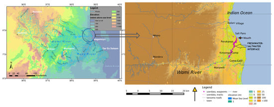
Figure 1.
Left—Wami River Basin in Tanzania. Right—the estuarine section on Wami River that starts from Matpiwili and Gama Gate, past Porokanya, flowing on towards the mouth at the Indian Ocean.
2.2. Hydrology and Water Quality
2.2.1. Historical Data on Wami River Flows
Data is available intermittently over 1960s–early 1980s and then since October 2006 for selected flow stations maintained by the Ministry of Water [48]. In addition, previous EFA studies for the Wami River in 2007 and 2014, a Rapid Ecological Assessment of the Wami River Estuary carried out in 2007; Ministry of Water, Government of Tanzania annual reports and the WamiRuvu IWRMDP documents. However, stage-discharge rating curves have not been updated since stations were installed in the 1960s.
The principal study site for the hydrological assessment was Gama Gate which is located just upstream of the saltwater–freshwater interface in the Wami Estuary (Figure 1 right). Although seawater does not reach Gama Gate (as evident from the freshwater riparian vegetation and water quality measurements), there is a possible tidal backwater effect as discussed later. Flows at Gama Gate had to be estimated based on the nearest station upriver with good historical records—Mandera station at Wami River Bridge. The missing values of the flow observations at Mandera station were previously reconstructed and infilled for the period 1955 to 1984 [48], hence, the reconstruction process was not repeated. The previous reconstructed time series data was used in estimating flows at Gama after accounting for seasonal flow contributions from the intervening catchment between Mandera and Gama and the water uses/abstractions, especially in the dry season (Supplementary Information Tables S1–S3). The intervening catchment was delineated from an ASTER Digital Elevation Model. Two considerations were taken in estimating flows for the Wami River at Gama Gate:
- (i)
- The flow contributions from the intermediate catchment during wet season: the period from November to May in the following year was relatively wet, constituting the short rains (October-December), the intermediate period/ transition period (January-February) and the long rains (March-May). In this case, a catchment ratio of 1.0324 was used to scale flow from Wami River at Mandera to Gama for the respective periods.
- (ii)
- Dry season abstractions for different uses: It was assumed that most of the water abstractions occur during the dry season (June–October). Hence, the total daily water abstraction rates were subtracted from the dry season flows at Mandera station and routed to Gama station. Note that the estimated water uses do not include “illegal” water extractions, such as those observed by us in the field.
Average monthly discharges were then calculated for wet, normal and dry years. A wet year is defined as a year with annual rainfall being one standard deviation greater than the average rainfall for the entire period. Similarly, a drought year has annual rainfall lower than one standard deviation from the mean annual rainfall over the period. The expected average monthly discharges in a normal year were computed using all years in which discharges were normal.
Flow duration curves (FDCs) were created from the obtained flow data—their shapes are related to the interactions of climate, catchment size and morphology, vegetation cover and the properties of the subsurface domain, which together control the various runoff components [50]. The FDC can be partitioned into three distinct parts [51], each of which is governed by different mechanisms or process controls:
- (i)
- The upper part, which represent high flows, is governed by flood processes for which the dominant control is the interaction of extreme rainfall and fast runoff processes;
- (ii)
- The middle part, which relates to the mean runoff and its seasonality, for which the dominant control is the competition and seasonal interaction between available water, energy and storage;
- (iii)
- The lower part, which is governed by base flow recession behavior over dry periods for which the dominant control is the competition between deep drainage and riparian zone evaporation.
In this study, the FDC percentage points were calculated from the average daily flow data at the Gama Gate. A substantial amount of uncertainty is expected in the quality of data used, since this data was extrapolated from Mandera as mentioned earlier; hence the FDC estimations are subject to the availability of data.
2.2.2. Hydraulic Channel Modelling, Tidal Backflow and Bathymetry
Field discharge measurements were carried out during the low flow season in August using a Q-Liner Acoustic Current Profiler at Gama Gate (BBM2), as well as further upstream at Matipwili (BBM1) and Mandera (Figure 1 right), sites where there have been Maji Bonde/Wami Ruvu Basin Water Office (WRBWO) staff gauges with data records since 1955 but with data gaps. The Q-Liner was operated from the edges to measure both the vertical velocity distribution and the water depth at every 1 m vertical positions. Since the flow sampling campaigns were conducted during the low flow season, the water depth was shallower than 1.2 m (Q-Liner’s minimum threshold) in some transects, thereby contributing to considerable uncertainty in discharge measurements. Since the flow depth was shallow during the fieldwork, the roughness condition was assessed visually using [52]. The coefficient of variation, Cv, for total streamflow, Q, as computed for all the EFA sites is less than 20%. In most practical applications, the Cv values are reasonably low to assume mean streamflow as best discharge for individual EFA site. Therefore, the mean streamflow was used as a steady upstream boundary condition in the hydraulic model for simulating the hydraulics.
The cross-sectional profiles of the river channel at Gama Gate and Matipwili were determined to relate water level (stage) with measured discharge, and thereby obtain a series of relationships between streamflow and other flow parameters including water depth, flow velocity, wetted perimeter and water surface width. Four river cross sections/transects were surveyed at each site (Figure 2 left and right) taking into account channel heterogeneity. Hydraulic data collected at each EFA site include cross-section geometry, reach lengths, water surface profile elevations, streamflow, flow velocity and roughness conditions.
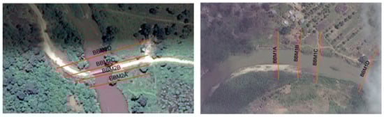
Figure 2.
Channel cross-section depth survey transects at Gama Gate (left) and Matipwili (right), Wami River, Tanzania.
The geometric survey entailed accurately locating riverine mesohabitat (riffle, pool, run, etc.), survey of bed elevation, and establishment of survey control points. A geometric survey at each EFA site was carried out at all channel cross sections using theodolites, a staff, and an 100 m steel measuring tape. The cross sections were placed perpendicular to flow. The geometry of the cross section within the main channel, below the water line, was surveyed using the manual water depth sounding approach. The measuring tape stretched across the channel width was supported from steel pegs (survey reference points) anchored on the banks. The cross section transects were in sections of the river where the mesohabitat is homogeneous across the channel. The study river reaches began with a downstream hydraulic control or riffle. The right bank and left bank were designated when looking downstream, with the left bank designated headpin and right bank designated tailpin. Verticals used in depth measurements were spaced at 1 m interval along the transect. Since the surveys were conducted during the low flow season, it was possible to access the riverbed and hydraulic controls. The conducted surveys provided information such as distance between transects, water-surface elevation, bed-elevation profiles, stage of zero flow elevation, water depths, and benchmark locations and elevations. The cross section transect extends beyond the Highest Flood Marks (HFM) to the cross-section freeboard. Existing survey benchmarks in the EFA sites were used as reference elevations. The benchmark used for the transect headpin and tailpin elevation surveys served as benchmarks for water-surface elevation (WSL) measurements during hydraulic data collection. Additional cross sections were identified and surveyed—they were sited at changes in water slope and channel geometry and along the bridge axis (see Figures S2 and S3 in Supplementary Information). The river longitudinal profile was required to determine the channel slope. Ideally this was supposed to be determined as the ratio of the difference between thalweg (deepest point) elevations to river reach length. However, considering the uncertainty involved in capturing the cross section deepest points, water surface elevation difference was surveyed and used with the assumption that a nearly normal uniform flow condition prevails. A survey of the left overbank and right overbank reach lengths was carried out using 50 m tape measure. The transects and general locations of the EFA sites were recorded using a handheld GPS.
Hydraulic Modeling: Hydrologic Engineering Center-River Analysis System (HEC-RAS) Version 4.1, a widely used one-dimensional hydrodynamic model for natural channel networks has been used as a modelling framework. Water surface profiles are calculated for steady, gradually varied flow. In model set up, it is necessary to divide the cross sections into parts that have homogeneous hydraulic properties, in the direction of the flow. These are usually the left/right overbanks and the main channel. It is assumed that there is no exchange of energy across the boundaries. Both the water surface elevation and the total energy head are assumed to be constant at the whole cross section. Such an assumption partly helps to reduce data requirements on observed water surface for calibration. Besides, in the field practice, it is difficult to capture the small changes in water surface elevation between the inner and outer banks at the meander as theoretically idealized. King et al. (2000) suggests that an ideal data set for EFA would be six data points of stage measurements over a wide distribution of discharges, plus the stage of zero discharge and some flood-related data. The EFA sites were assessed for only one sampling event conducted in August 2015. Therefore, to interpolate or extrapolate hydraulic parameters other than the measured ones, a reach-based HEC- RAS hydraulic model was set up for the two EFA sites. The model uses Manning and energy equation(s) to simulate river hydraulics. Quantitative and field observation data were used to calibrate and validate, respectively, the flow parameters (hydraulics) simulated by the hydraulic model. The parameters include maximum water depth, flow velocity, flow area, wetted perimeter and top water surface width. The model was calibrated by matching the simulated and observed water surface profiles as they are considered most reliable. Model performances for other pertinent simulated hydraulics such as velocity, wetted width, flow area, etc., were evaluated qualitatively and quantitatively. Quantitatively, the model performance was considered satisfactory for relative error at less than 20%. Then, the validated model was used to simulate the hydraulics in a range of stream that mimic drought, medium, and bank-full flow conditions.
Backwater tidal effects at freshwater end of estuary: The water level in the river at both Gama and Kinyonga was observed to be falling from mid-morning through the early afternoon, leaving a moist band of 25–30 cm on the riverbank soil. The river level rose again early evening onwards. This periodic rise and fall were likely an effect of the freshwater flow backing up during high tide (although diurnal changes in level can also partly result from evapotranspiration of the surrounding gallery forest). Flow measurements were made periodically (about every 5–10 min—Figure S4 in Supplementary Information) between 10 a.m. and 5 p.m. on the surface at Gama Gate and Kinyonga on two separate days using a mechanical current meter (Model 2031, General Oceanics, Miami Gardens, FL, USA). Additionally, at Gama, water depth was also recorded.
The method to determine a bathymetry map of the river estuary is included in Supplementary Information.
2.2.3. Water Quality
Boat-based measurements of water quality parameters were done in neap tide season between 20–24 August 2015 during flood and ebb tides. Water temperature, salinity, dissolved oxygen, electric conductivity and total dissolved solids (TDS) were measured by using handheld EC and DO probes (YSI EcoSense EC300A and YSI EcoSense DO200A, YSI, USA). Cables with EC and DO sensors were tightly tied in a calibrated pole for easy measurement of parameters at depths of 1 and 2 m. Water clarity was measured by using a 30 cm diameter Secchi disk while pH was measured using BANTE 900P portable multi-parameter meters. Water from 1 and 2 m for pH measurement was collected by a small water sampler of 400cc. Measurements were taken during ebb tide from the surface every kilometer from upstream of Kinyonga site towards the river mouth. Measurements were repeated during flood tide from the Ocean going upstream to Kinyonga. Since tidal conditions changed a lot when sampling over the entire length of the estuary, water quality measurements were taken at four sites for consistency and comparison. Site 1 represented the river mouth (the lower estuary), site 2 and 3 represented the mid estuary whereby site 2 was characterized by a very sharp corner/meandering, and site 3 was the transition zone of mangroves to palms. Site 4 represented the upper estuary at the extent of the tidal limit.
2.3. Riparian Vegetation Zonation—Multi-Decadal Indicator of Salinity Regime
The plant species composition of a riparian forest is tightly coupled to the seasonal flow regime of the river and offers clues on the extent of flooding of banks, soil water availability and salinity occurring in the root zone (rhizosphere). An earlier report on the Wami Estuary [45] described riparian vegetation zonation into three dominant plant communities based on salinity tolerance:
- (i)
- Saline water vegetation—dominated by mangroves;
- (ii)
- Brackish water vegetation—dominated by the palms Nypa fruticans/Phoenix reclinata and some mangrove species;
- (iii)
- Freshwater vegetation—dominated by Ficus-Kigelia-Terminalia in the canopy with herbaceous annuals and wetland vegetation on sandbanks that are inundated over the wet season. This zonation indicates the long-term salinity regime (over several generations of trees), and hence affords clues to both wet season freshwater flooding as well as the extent of seawater intrusion upriver in the dry season.
Vegetation on riverbanks was observed on all boat trips along the estuary and identified to the species level. Species were recorded with GPS points and mapped, notes taken in reference to salinity and water level, as well as riverbank morphology (whether erosional or depositional, that also indicates vegetation succession and extent of flooding in the wet season). Special attention was given to the locations and nature of transitions of major vegetation types, such as palm–mangrove. No shore landings were made (except at Porokanya, Kinyonga and Gama). Onshore transects were not possible on account of the presence of hippopotami and crocodiles.
2.4. Aquatic Ecosystem, Terrestrial Wildlife and Human Water Use
2.4.1. Fisheries Survey
A rapid field survey was conducted for five days (19–24 August). Two methods were employed: (1) boat-based fishing in the estuarine part of the Wami River and (2) visiting nearby fishermen’s landing sites. A 2 m-wide and 100 m-long gillnet with stretched mesh size of 1.5 inch was used for fish sampling. The net was set in the deeper part of the channel while making a cycle; fish were then trapped, encircled and collected. Fish individuals caught were identified to species level. Prior to fishing, environmental parameters (salinity and temperature) were measured in the estuary. Two fish landing sites at Kajanjo and Saadan villages were visited. During visits, we observed fish landings (catch) from fishermen and conducted discussions with a few fishermen on the trends of the fishery. Species caught from fishers was identified to species level; other information noted were type of the gear and vessel used. In addition, findings from the literature search, field survey and catch landings from fishermen were used to assess the water needs for fish and associated aquatic organisms in the Wami Estuary. Data are provided in Supplemental Info.
2.4.2. Terrestrial Wildlife Survey and Water Requirements
The tidal and seasonal variation in the fresh and brackish reaches of the river affects the distribution of wildlife; for example, colobus monkeys, hippos, elephants, crocodiles, wildebeests and bucks use water from the river along different points, since these animals differ in the degree of brackish water they can tolerate. The abundance and diversity of bird species are connected with estuarine habitat heterogeneity, as some birds are usually found on sandy beaches, others on edges and in mangroves, palm trees, grasslands and wooded grasslands upstream the river. The analysis relies on a literature review, the experience of the SANAPA staff and field work in the current study. A transect of about 24 km was covered from the river mouth passing through mangrove forest (4.72 km), mangrove–palm transition zone (0.73 km), palm forest dominated by wild date palm—Phoenix reclinata (2.71 km), palm–riparian transition zone (0.51 km) and freshwater riparian vegetation (14.57 km). The aim was to record the habitat changes and wildlife species found in the Wami Estuary. On account of the rapid nature of the field assessment, there were no exact times used for recording wildlife species in the field; instead observations were made while travelling up and down the estuary during both high and low tides. Wildlife species (birds, large reptiles and mammals) were recorded based on area observed followed by location, habitat type and number of individuals found at that point, but small reptiles, amphibians and invertebrates were not possible to be recorded on this boat-based survey. Amount of water consumption required by each species and population was estimated based on the body size of the animal and by using literature available showing the amount required per individual for some species also used to estimate to other species corresponding to those sizes (Supplemental Info).
2.4.3. Human Resource Use—Water, Farming, Forests, Fisheries, Tourism from Wildlife
The socioeconomic component of the Wami Estuary study aimed at documenting the human uses of ecosystem services in the Wami Estuary. It further assessed community perception on future existence of these resources. Study sites were two villages, Kitame and Saadani, within the Wami Estuary. Saadani village, located inside the Saadani National Park, has a population of 1606 people, while Kitame village, located south of the estuary, has a population of 1452 people. The interviewed population was around 90 people. Data was derived from extensive review of literature, key informant interview, focus group discussions and field observation. With assistance from staff of the Saadani National Park, the social scientist spent some time with communities, conducting focus group discussions with different groups of men, women, youth and elders. She also interviewed key informants, namely representatives from the Saadani National Park, Sanctuary Saadani Safari Lodge, Saadani River Lodge, salt industries, farms along the Wami River, village leaders, fishermen, and wise elders (Supplemental Info).
2.5. Environmental Flows Determination
The approach for the Wami Estuary EFA was based upon the widely used Building Blocks Method (BBM)—[53] where the magnitudes and necessity of flows in a river during different seasons are linked with various life-supporting processes in the aquatic ecosystem in that river. The range of water flow necessary to maintain a certain ecological process is thought of as a “building block”, with blocks added over each other across seasons to visualize the flow necessary in a river for various ecological needs [54]. The flows necessary for different ecosystem processes were identified by the experts to the best of their knowledge, given the paucity of data relating flora and fauna communities to flow and salinity in the Wami Estuary, or coastal East Africa in general. The process of determining the environmental flows (freshwater inflows) for Wami Estuary followed these steps:
- Presentations on the state of knowledge and fieldwork results for different components of the study—ecosystems (aquatic, riparian, terrestrial), human resource use and hydrology of the estuary.
- Decision on the present ecological state of each ecosystem component, the trajectory of change, and the desired target for restoration/maintenance with the assignment of Grades A–F (Table 1).
 Table 1. Summary of the ecological categories used in determination of the present state and for the recommended ecological management class.
 - Determining the minimum depth necessary to prevent disappearance of various ecosystem components. This was done for the dry and wet season. Apart from minimum depths, the role of flood pulses along with their magnitudes were also noted.
- Confidence estimates for each EFA component.
- Obtaining flow or discharge values from corresponding minimum depth values using a hydrological model developed for relating depth to discharge at Gama Gate.
- Extrapolation of these values for other months to obtain a minimum set of environmental flow recommendations for each month, as measured at Gama Gate. This was done in a manner that replicates the seasonal variation inherent in the historical flow average data.
- Comparison of the recommended EFs with the historical flow data, to see how achievable these recommended minimum flows are.
2.5.1. Characterizing the State of the Ecosystem
Based on these three conditions, each expert offered a suggested Ecological Management Category (EMC) for each site, scored between A through D. SANAPA staff and director, WRBWO staff and particularly the Basin Water Officer as well as the Water Engineer from Bagamoyo District contributed information on the management challenges they face at each site, historical conditions and on potential developments—such as dams or irrigation projects—that might be on the horizon. Based on these discussions, a consensus recommendation for Ecological Management Category (EMC) was made for the estuary ecosystem.
2.5.2. Linking Ecosystem with Hydrology
Flow recommendations to achieve the suggested EMC in the estuary were made using a combination of information from the published scientific literature, field data and professional judgment. The process for setting flow recommendations generally followed that outlined in BBM [55]. The experts were asked to consider the flow needs as related to ecosystem structure or ecosystem function in six different scenarios: 1. Low flow in the dry season of a drought year; 2. Low flow in the wet season of a drought year; 3. Low flow in the dry season of a maintenance year; 4. Low flow in the wet season of a maintenance year; 5. High flow in the wet season of a drought year, and 6. High flow in the wet season of a maintenance year.
Additionally considered was the ecological role, the magnitude, and the timing of floods and peak flows. All the flow suggestions were backed up with detailed, written descriptions of the objectives of different kinds of flows—for instance, a high flow in the wet season—and the experts’ professional motivations—based on field data or knowledge from the literature—for recommending these different flows during different seasons. Standardized flow objectives and motivations forms were completed by the respective scientists during the workshop. In some cases, for instance, for the aquatic ecologist and riparian ecologist, it was easier to identify the habitat conditions associated with indicator species—such as velocity or depth—rather than try to recommend flows in cubic meters of water per second; in these instances, the hydraulic engineer provided the corresponding flows for these parameters from a hydrological model created and configured for the channel at Gama Gate. The hydrologist looked back in the historical record to verify whether these recommended flows were within the range in the historical data, and thereby, possible.
A consensus was thus reached for a recommended environmental flow for the dry and wet season conditions in drought and maintenance years and for floods. Each expert suggested flow recommendations by discipline and was asked to defend the reasoning behind those recommendations. Each expert also estimated a level of certainty that the recommended environmental flow would satisfy the needs for species or important ecosystem processes, like sediment transport. The discussion for each site was concluded only once a consensus for flow recommendations had been met, a facilitated process that typically lasted about two–three hours. The hydrologist then took the recommendations for the dry, wet, drought, maintenance, and flood conditions and extrapolated them across the year, following the BBM [55]. The resulting information constituted a prescribed environmental flow regime for the estuary taken at Gama Gate.
2.6. Montana or Tennant Method
This method [35] recommends maintaining 10% of the average annual flow as a minimum instantaneous flow to sustain short-term survival habitat for most aquatic organisms, 30% average flow as the base flow to sustain good survival and 60% average flow to provide excellent conditions for growth of most aquatic life forms and most recreational uses. Furthermore, this method divides the year into fish spawning season and regular maintenance periods (April–September and October-March), specifying flow requirements as percentages of mean annual flow for a series of river ecological conditions, from natural unmodified to highly modified/degraded. In this study, the mean annual flow obtained at Gama Gate is utilized for the Montana method.
3. Results
3.1. Wami River Inflows to the Estuary—Historical and Field Data
The results from long term analysis of flows and rainfall indicate the existence of a well-defined peak in Wami River flow during the wet season and low flows during the dry period, namely July to October (Figure 3). In a normal average year, monthly average discharges vary from as low as 15 m3/s usually recorded in October to as high as 186.3 m3/s in April. In dry years, average monthly discharges ranges from 9.9 in November to 79.8 m3/s in April. The daily flow hydrographs for wet, normal and dry years (Figure 4) indicate high flows during the April–May as well as a fair amount of variability or flashiness as a response to rainfall in the Wami Basin. The ecosystem in the river and estuary has evolved with this large variability of flow within a typical year, which is a very important aspect to be kept in mind while managing water abstractions and maintaining flow within the river. The daily flow duration curve at the Game EFA Site (Figure S1, Supplementary Info) reveals gradual sloping indicating stable flows in the river. For most of the time (between 40–60%), the flows are around the mean. The summary of maximum flow quantiles at Gama are presented in Table S4, Supplementary info.
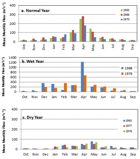
Figure 3.
Mean Monthly Discharge (m3/s) in (a) normal, (b) wet and (c) dry years at Gama Gate, Wami River, Tanzania.
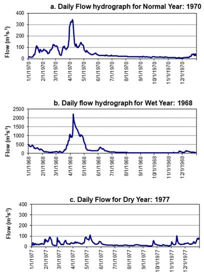
Figure 4.
Daily flow hydrographs (m3/s) for (a) normal, (b) wet and (c) dry years at Gama Gate, Wami River, Tanzania.
3.2. Channel Cross-Section and Hydrological Model
The channel cross-sections at the four sections in each of the two sites are shown in Figures S2 and S3 in Supplemental Info. The model performance for the five flow parameters—mean velocity, water surface profile elevation, flow area, water surface top width and maximum water depth was evaluated quantitatively based on the relative error in percentage criterion (Tables S5 and S6, Supplementary Info). Generally, model performance was found to be satisfactory in most of the transects. The transects with very good performance are recommended for use in the EFR workshop. The results from other transects need to be used with caution as professional judgment is critical for meaningful application.
Simulated water surface profiles: The hydraulic model simulations developed a series of relationships between streamflow and other parameters such as maximum water depth, flow velocity, flow area, wetted perimeter and water surface width. Figure 5 shows the water surface profile plots for the selected transects. The hydraulic river reaches of EFA sites capture the variability in habitat types and hydraulic regimes. The width of the macro channel ranged from 34 m to 40 m. The longitudinal water surface profile slopes are 0.0003 and 0.001 for channel transect sites BBM2 and BBM1, respectively (Figure 2). This result indicates that two sites are situated in distinct geomorphologic zones and/or hydraulic regimes. The product of this component comprises of a series of relationships between streamflow and other flow parameters such as maximum water depth, flow velocity, flow area, wetted perimeter and water surface width. Errors spotted in hydraulic simulations are attributed to uncertainty in discharge measurements, lack of the original bridge design data, complexity of the river geometry and the influence of backwater flow from the sea at BBM2 site in Gama. Furthermore, fieldwork data were collected during the low flow season in August, but the driest month in the study area is November. The hydraulic model is based on only that one sampling event. It is therefore recommended that the hydraulic model be validated with high-flow-season data. Additionally, the low-flow data may be revisited during the driest month with the use of current meter or a Q-Liner model with a lower minimum depth threshold.
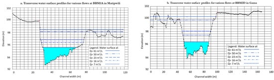
Figure 5.
Channel cross-sections and simulated water surface profiles for different flowrates at (a) Matipwili and (b) Gama Gate, Wami River, Tanzania.
3.3. Water Quality—Salinity Spatial Profiles during Flood and Ebb Tides
As salinity is the main water quality parameter required for understanding freshwater and seawater dynamics, other parameters while measured are not included here (but are provided in Supplementary Info). During the sampling period, the lower estuary (5 km from mouth upriver, corresponding to the mangrove zone) was mainly freshwater-dominated (0.1–0.3 ppt) at ebb tide (Figure 6 bottom) and saline water-dominated at flood tide (Figure 6 top). Saltwater intrusion extended up to the area of mangrove/palm transition zone during flood tide, showing different patterns of mixing and stratification through the water column (Figure 6 top). Homogeneous mixing occurred at site 1 and site 4 on 23 August 2015 while the mid estuary showed partial stratification through the water column with surface salinities of 17.1 and 1.1 ppt and bottom salinities of 25.6 and 7.3 ppt at site 2 and 3, respectively. On 24 August, strong stratification was observed at site 1 with surface salinity of 13.1 ppt and bottom salinity of 31.7 ppt (Figure 7 top). Partial stratification occurred at site 2 with surface salinity of 6 ppt and bottom salinity of 10.4 ppt, while the other sites were homogeneously mixed with salinity of 0.4 and 0.1 ppt throughout the water column at site 3 and 4, respectively (Figure 7 bottom).
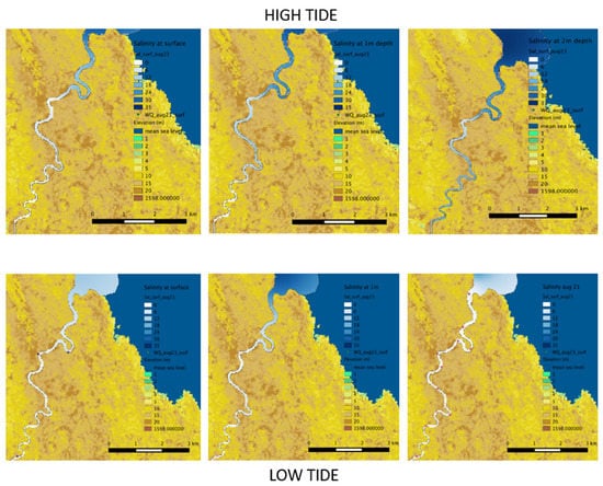
Figure 6.
Salinity profiles in the Wami Estuary: Top panel shows salinity at surface, 1 m and 2 m depths during high tide (23 August). Bottom panel left and center shows salinity at surface and 1 m depth during low tide (23 August). Bottom panel right shows salinity at the surface during low tide on 21 August. Deeper blue indicates higher salinity (upper legend from white to blue in each map). Lower legend indicates land topographic elevation.
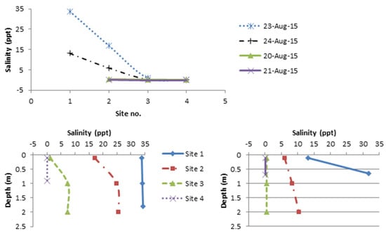
Figure 7.
Top—Surface salinity profiles upstream from estuary mouth (sites 1–4), with Site 1 being at the mouth. Bottom—Depth profile of salinity during flood tide (23 Aug-15—left) and (24 Aug-15—right).
Because the ocean site was sampled only once, we did not observe a clear demarcation of freshwater plume at low tide as it was observed in August, 2007 [45]. The ocean had salinities of 34.1 ppt at the surface and 34.2 ppt at 1 and 2 m depths. Salinity recorded after site 3 towards the upper estuary during both ebb and flood tide were similar to salinity recorded in August 2007, i.e., 0.1 ppt. The rest of the river from site 4 to Gama Gate was mainly freshwater with salinity of 0.1 throughout the water column during flood and ebb tides. However, in times of very low freshwater flows, particularly in October, salinity intrusion extends beyond the site 4 and sometimes up to the newly constructed water supply pump for Saadani village. For example, in October 2007 during high tide, salinity at site 4 was 10 ppt at the surface and 17 ppt at the bottom (Kiwango’s PhD fieldwork). The villagers of Saadani also have been complaining about having saline water which is undrinkable from the water supply tank during high tides, especially during spring tide.
3.4. Riparian Vegetation Zonation
Seven mangrove species were observed in the Wami Estuary with varying known salinity tolerance ranges (Table 2). Sonneratia alba (SA) and Avicennia marina (AM) are the most salt-tolerant of the mangroves; in addition, SA can tolerate continual inundation in seawater for the longest period. Both SA and AM have pneumatophores as an adaptation to prolonged immersion in waterlogged soils. Hence, monodominant stands of SA occur on the river mouth, closely followed by AM. Rhizophora mucronata (RM) also tolerates 30–35 ppt seawater, as seen by occurrence of RM with stilt roots along banks that are regularly inundated at high tide. Ceriops tagal (CT) and Xylocarpus granatum are less salinity-tolerant and grow on banks that are higher, limiting the inundation exposure to seawater. At the lower end of the tolerance scale lies Brugeria gymnorhiza (BG) and Hereteria littoralis (HL) that occur further away from seawater channels. More information on mangroves and riparian plant community structure in Tanzania can be obtained in [44,49,56,57].
Table 2.
Mangrove species occurring in Wami Estuary, Tanzania.
Figure 8 shows a vegetation schematic map of the estuary, resulting from this fieldwork. At the river mouth, Sonneratia alba dominated the coastal margin, including sandbanks with lone individuals. Close behind the shore were monospecific stands of Avicennia marina. These banks get tidally inundated. In addition, the extent and duration of inundation is larger during spring tides as compared to neap tides, as well as in the rainy season when higher freshwater flow in the river leads to higher water levels overall. A slightly higher bank (<1 m at high tide) had individuals of Rhizophora mucronata inundated at high tide, with few Bruguiera gymnorrhiza and Ceriops tagal higher on the bank (not inundated). Thereafter follows a zone of Xylocarpus granantum with curly ribbon roots on the mudbank, which dominates a large part of the estuary before giving space to Heritiera litoralis close to the transition zone. While Xylocarpus and Heriteria are dominant canopy species, the bank shore and sand depositional areas at river bends were dominated by stands of Avicenia, and at times Sonneratia. Difference in mangrove species composition on either bank of the river is likely a result of the differences in bank height. This is especially noticeable at river bends, where the convex bend has sand deposits and is thereby much lower than the opposite bank, which is scoured and hence steep. The lower bank gets flooded more frequently and for longer periods than the higher bank, resulting in flood-tolerant mangrove species (Avicennia) on the sandbanks. Figure 8 indicates the occurrence of different species of mangroves as well as other species, whose locations were recording using a handheld GPS.
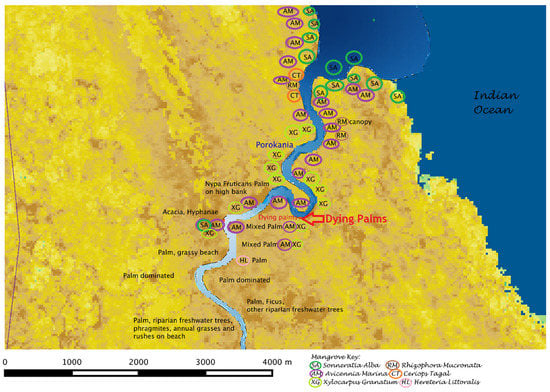
Figure 8.
Vegetation map of Wami Estuary; deeper blue in river channel indicates increasing salinity. Please refer to Figure 6 for salinity legend.
Palm-mangrove transition: At the transition zone, the mangroves Xylocarpus, Avicennia and Sonneratia give space to palms on the riverbanks (either Nypa fruticans or Phoenix reclinata, or perhaps both) which dominate further upstream about 1.5 km (Figure 8). These palms can tolerate flooded soils and slightly brackish water. In August, salinities at flood tide were less than 5 ppt at the river bottom in this zone. Hence, the mangrove–palm transition zone has been widely held to demarcate the extent of seawater intrusion on average [45,49]. While there are episodes when seawater intrudes further upriver (as noted by the Saadani village water supply project situated another 4–5 km upstream that could pump water only at low tide), the seawater would be flowing in along the bottom, overlain by freshwater which is what the plants would be accessing. In addition, relatively less salt-tolerant mangroves on high banks would also be likely utilizing a soil-rainwater pool in the rhizosphere. For instance, in the estuarine section of the Florida Everglades, a perched rainwater pool allows salinity-intolerant trees (such as Conocarpus erectus, Eugenia fetida, Bursera simarouba, and Swetenia mahagoni) to coexist with mangroves over the regional saline groundwater, albeit on slightly higher locations on the order of as little as 10–15 cm [58]. In addition, high freshwater inflows over the successive wet season can flush out some of the salt that might remain in the soil pores.
Freshwater riparian forest: At the upstream end of the transition zone (Figure 8), about 6 km upriver from the mouth, the mangroves disappear and are replaced by palms and salinity-intolerant trees dominated by Ficus sycomorus, Salvadora percica, Kigelia and Terminalia species, reaching canopy heights up to around 10 m. Other palm species, Hyphaene compressa and Borasus sp were seen in this zone, however these palms occurred inland, and not on the riverbank. Several species of climbers were commonly seen in Palm trees, at times forming thickets. Along river bends, the beaches are colonized by herbaceous annuals and wetland vegetation (rushes, reeds, Cyperus papyrus and grasses including Phragmites)—indicators of seasonal flooding that do not allow woody vegetation to establish. The herbaceous annuals die back every year when continuously flooded by high water levels for several months in the wet season. Wetland vegetation have root and stem adaptations to withstand saturated soils. Woody vegetation, such as mature trees, occur beyond this belt of herbaceous plants, thus indicating the extent of flooding on average over the past decade at least. Further inland, away from the river in the Zaraninge forest [59] exists savannah woodland dominated by Acacia zanzibarica along with A. nilotica, A.melifera and Dichrostachys cinerea interspersed with open grassland dominated by Sporobolus sp. mixed with few unidentified shrubs. Figure 9 summarizes the plant community types in relation to the river salinity regime as observed during this fieldwork in 2015. Salinity at high tide is depicted in this figure to indicate the extent of salinity intrusion.
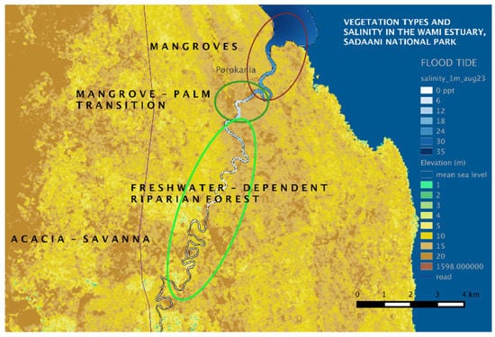
Figure 9.
Plant communities in the Wami Estuary, Tanzania, with relation to river salinity; salinity at high tide in August is shown.
3.5. Coastal Habitats and Fish Survey
The lower salinity in estuaries attracts large numbers of juvenile prawns, with different species preferring different habitats. For example, Peneus indicus is found on muddy and mangrove-lined regions, while Peneus latisulcatus appears to prefer sandbanks with seagrass growth [60]. The presence of a 10–30 cm mud layer on the seabed at the mouth of the river suggests that any seagrass beds that may have been there have been smothered in sediment. Seagrass beds were observed a half kilometer away from the river mouth along the coast, with seagrasses of several species regularly washed up on beaches on either side of the Wami Estuary. The area around Wami Estuary is known as one of the most productive prawn fishing grounds in Tanzania—classified as fishing area Zone I as per TAFIRI [60]. The prawn fishery was closed in 2007 following the decline in the industrial catch, however, artisanal fishing is still operating [61]. The dominant fishery in Saadani area was and still is prawn fishery with peak season from March to April [62]. Overall good agreement between fishermen’s perception was that Saadani used to be the ground for prawn fishery, but changes in the water flow and other environmental parameters has resulted in the collapse/decline of the prawn fishery. This decline over the past three decades has also been noted by Silas (2011) in his review of Tanzanian prawn fisheries.
The most common fish species that inhabit the Wami Estuary are Arius africanus, Hilsa kelee, Liza macrolepis, Chanos chanos and Thryssa spp. Crustaceans includes Scylla serrata, hermit crabs, and prawns. Molluscs include Saccostrea cucullata, Terebralia palustris, Cerithidea decollata and Strombus spp. Moreover, there are a number of freshwater fish species that inhabit the freshwater part of the Wami basin. These species can potentially move downstream during rainy season [63]. The most common fish species caught during this survey (Supp. Info Table S10, Figures S10 and S11) includes: Arius africanus, Valamugil buchanani and Thryssa baelama. Crustaceans include Scylla serrata and hermit crabs. At the river mouth, the dominant species was African catfish (Arius africanus); the same species was observed in large numbers at Fungu Maboko. A few kilometers away from the river mouth upstream at Saadani River Lodge, the catch was mainly dominated by Valamugil buchanani, the same species came second at Fungu Maboko. The situation was different a few kilometers offshore, where there was a large variation in species caught, with puffer fish (Tetradontidae) being the dominant fish. There were 18 different types of fish species observed at Kayanyo landing site and 10 species at Saadani. The catch was mainly dominated by prawn species (Paneus monodon) in Kayanyo and Indian pellona fish species (Pellona ditchela) at Saadani landing sites. This could potentially indicate diversity and abundance of fish species decrease as the distance from river mouth increases. However, the opposite situation could possibly occur during large floods in the rainy season as freshwater inputs pushes away marine water. Year-round sampling of fish catches can yield more information as to the abundance and diversity of fish species in the estuary and surrounding coastal and upriver areas.
3.6. Habitat Types and Distribution of Birds, Reptiles and Mammals along the Estuary
The distribution of birds, reptiles and mammals were influenced by habitat type and water conditions. Habitats along the Wami River estuary have been identified and categorized into five areas, namely, mangrove forest, mangrove–palm transition zone, palm forest, palm–riparian transition zone and freshwater riparian vegetation. Detailed results from the wildlife field and literature surveys are included in Supplementary Info. About 28 bird species were observed with woolly necked stork, little bee-eaters and golden weavers being most commonly seen along the river (Supplementary Info Figure S9, Table S12). Only large reptiles (Nile crocodiles and green monitor lizards) were observed on this boat-based survey study. Hippos are living under their minimum water depth level due to low freshwater inflow in the river channel, and they aggregate to small parts of high depth and entirely rely on fresh water, although few groups tolerate low salinity maximum of 5 ppm at the mangrove environments during high tides (Supplementary Info Figure S8). Primates such as the Black and White Colobus monkey and Blue monkey rely on freshwater, specifically to palm and riparian environments, which are threatened by both invading salinity and human disturbances such as clearing riparian vegetation for cultivation. Increasingly large freshwater abstractions from Wami River in the estuary endangers hippos and crocodiles as it decreases the surface water required for these species to survive during dry season. Large herds of cattle accelerate soil erosion along the riverbank. The high wildlife diversity in the Wami River estuary and SANAPA depends upon adequate freshwater inflows in the Wami River, as well as the protection of the riparian vegetation along both banks of the Wami River estuary.
Water Requirements for Wildlife
The Wami River is the only perennial source of water for both terrestrial and aquatic wildlife in Saadani National Park, apart from a few pools constructed by the Park Authority. Table S11 (Supplementary Info) indicates the estimated amount of water required per population found in Saadani National Park. The abundance of large-bodied mammals such as African elephant, African buffalo and Masai giraffe in the park is relatively low; however, the volume of water required per day by these large mammals is high compared to small and medium size mammals (Supplementary Info Figure S9). In Saadani National Park, the elephant population requires the most water (190,000 litres) while the buffalo population consumes around 140,000 litres, and the giraffe population around 71,000 litres per day. The movements of African buffaloes are influenced by water availability, especially during dry season, when they are never found very far away from water sources. Some elephants and buffaloes are often seen crossing the Wami River and drinking water during the dry season on upper regions of the river between the Matipwili area and Gama gate. Giraffes are mostly found in acacia savanna browsing leaves and they prefer to be close to water sources as well. Waterbucks and Hartebeests are also very common around water sources and their consumption of water is intermediate as shown in Table S11, Supplementary Info. Yellow baboons seem to require a high amount of water compared to other primates; most of the time they are found on the open grassland eating stems of palatable grasses with high sugar content which in turn causes baboons to drink water. Despite individual baboons drinking infrequently, their large population has a cumulative high demand for water—around 33,000 litres per day. Although they are small in body size, they are the largest population in the park, and even their water requirement is still high compared to some large-medium bodied mammals.
Some animals consume relatively low amounts of water due to low population and small body size, but they are highly influenced by habitat type. For instance, blue and black and white colobus monkey has been occasionally sighted drinking water from the river, and more commonly from water trapped in hollows in trunks and flowers in the riparian vegetation. These arboreal monkeys also feed on invertebrates trapped in these water pools. Hence, the palm and riparian forests, so dependent on the river water levels as well as intolerant of salinity are critical for shelter, food and water for these primates. Palm forests also provide nesting sites for numerous bird species as well as supporting reptiles and insects, which are part of the gallery forest food web.
Hippos are large-bodied mammals that require a minimum depth of water for reproduction as mentioned earlier. The current levels of water in the mid-dry season in the Wami are insufficient for this. Hippos usually mate in the wet season; however, the females can conceive year-round. Only the dominant male in the group can mate, and hence the restriction of mating opportunities due to low water levels can significantly affect reproduction. A female generally only has one offspring every two years. Another concern of low water levels is sunburn and peeling skin for female and baby hippos that happens in shallow water. The range of water depth at Gama gate in the mid dry season (20–22 August) was from 0.76 m at low tide and 1.18 m at high tide while the favorable depth range for hippos is 1.5 m to 14 m (Estes, 1992). Therefore, at low tide, hippos tend to migrate downstream and during high tides, they avoid too much salt water and move to upstream areas with moderate depth from palm forest upstream up to about 2.5 kilometres after Kinyonga camp site. When water depth is below 0.15 m, hippos desiccate [64] and hence migrate to deeper areas. This could be the reason for hippos to not reach Gama gate that often (where it is shallower than downstream) although their trails going to and from grazing are visible on the bank. Behaviorally, male hippos select females who are in heat, chasing the females back to water with high depth for mating; the female has to be totally submerged [65], hence, if the depth of Wami River continues to decrease downstream, hippos will lose mating sites, thus affecting their reproduction. The literature points out that combination of natural and human disturbances to hippos’ population can cause them to disappear within 60 years [66] and that hippos are declining on the range of 7 to 20% over past 10 years while the estimated population of hippos in the world is about 125,000 to 148,000 individuals in 29 countries [67], hence, hippos are very sensitive to human disturbances like water level changes due to large abstractions, erosion caused by cattle, habitat loss due to grazing and cultivation near the Wami River. During the day, hippos remain in shallow water for mating and raising offspring, emerging only in the evening to graze for a distance of not less than 1.6 km along the river banks [66,68,69]. Cattle rearing and cultivation activities affect their livelihood by competing for grass, causing hippos to migrate.
3.7. Human Use/Dependence on Estuarine Ecosystem Services
The Wami is the only source of freshwater for village domestic needs and for international tourist lodges in the estuary. Vegetable cultivation (including tomatoes, watermelon, spinach, green peppers, and bananas) relies on dry-season irrigation using river water via portable water pumps (5.5 hp). Migratory pastoralists have been recently arriving in Kitame village with several herds 300–500 head of cattle per herd); they depend on the Wami River and nearby ponds as sources for providing water for their cattle. According to studies, highland dairy cattle use about 36 m3/head/yr., upper basin dairy and beef cattle use 27 m3/head/yr., and lowlands cattle use 18 m3/head/yr. [70]. Fishing is a major livelihood activity within the estuary and a major source of food for most of the people in Saadani village and coastal areas. Mangroves have long been harvested and used as poles for housing, firewood and charcoal for fuel, medicine, boat building and raw materials for fishing gear. The high demand for resistant wood from mangroves has led to its overexploitation, making management and protection of these forests even more important. Construction of evaporation ponds for solar salt production is another threat to mangroves, where 75% of salt in Tanzania is currently produced via solar production [63]. Despite their ecological importance of stabilizing shorelines from wave and storm erosion as well as habitat for the fish and invertebrates, human utilization of mangroves is very high, with the most destructive activities being clearing of mangrove for salt pans and charcoal production. The Wami River is the only reliable source of water for wildlife in Saadani National Park. International wildlife tourism is a major source for income to local communities as well as Tanzania as a whole. Generally, there has been a decline in almost all riparian resources in recent years as reported by interviewed communities. The major reasons as mentioned by villagers were climatic change being linked by unpredictable rains, increased temperature and the rise in sea water level. Human activities such as tree cutting for timber and charcoal making, land clearing for agriculture, illegal fishing, bush fire, illegal mining, and unsustainable use of water irrigation activities were reported to be the contributing factors.
3.8. Environmental Flows Workshop
3.8.1. Status of Ecosystems
The experts evaluated the current state of their respective ecosystem component (Table 3), assigning a grade and explaining the reasons for their assessment. The lowest grade assigned is taken to be the overall state of the ecosystem. In the case of the Wami Estuary ecosystem, the overall status was deemed to be C.
Table 3.
Status of various ecosystem components in the Wami Estuary.
3.8.2. Trajectory of Ecosystem Change
Experts assessed the direction of ongoing change (Table 4: options are positive, no change and negative). Changes over the past decade as well as the present trajectory were seen to be negative. For instance, in the mid-2000s, there was much less turbidity and sedimentation in the estuary as compared to the present. Furthermore, as the basin wide demand for water, together with increased agriculture, deforestation and soil erosion occur, if not controlled or managed effectively, the outlook is lower freshwater inflows coupled with higher sediment and agrochemical loads.
Table 4.
Trajectory of change in various ecosystem components.
3.8.3. Desirable Ecosystem Status—The Extent to Which the Ecosystem Can Be Restored and Maintained
While establishing a minimum set of freshwater inflows that are needed to sustain the estuarine ecosystem, it becomes necessary to decide in what state the ecosystem should be maintained. The goal is to understand what level of ecosystem structure and function is essential to maintain critical ecosystem services such as marine fish nurseries, wildlife habitat and maintaining riparian forests. Table 5 summarizes the assessments from the team. Ideally the goal would be to restore the ecosystem to the pristine state, prehuman disturbance, i.e., grade A. However, such a state is impractical given the considerable human presence in the basin. The challenge is to maintain critical ecosystem functions amidst increasing human resource demand and impacts. The team’s decision was to strive for a grade better than a B, which is B +, which is also reflective of the tremendous ecological importance attached to the only protected estuary in Tanzania as well as regionally along the eastern coast of Africa.
Table 5.
Restoration goals.
3.8.4. Consolidating These Assessments
For each season–flow–year combination, the minimum depths required were evaluated by the team, and the largest value for the minimum depth was selected as the critical ecosystem MINIMUM depth value. Going below this minimum would lead to mass mortality and the rapid, catastrophic failure of key ecosystem processes, from species reproduction to food web cascading effects to biogeochemical cycling. Individual results for the six cases are included in Supplementary Material. Water depth was chosen instead of water flow, as for most ecosystem components it is easier to relate quantitatively to water depth as opposed to flow (whose values are not known if not measured, and additionally, flow speeds change with depth). Furthermore, for riparian vegetation, water depth or river water level controls the depth of the water table and unsaturated soil zone that dictates water availability to plant roots. The hydraulic engineer obtained the discharge value corresponding to a given water level from a hydrological model set up with the cross-section geometry at Gama Gate (Table 6).
Table 6.
Summary of minimum discharges and corresponding minimum water depths necessary at Gama Gate for the 6 different hydrological conditions to avoid ecosystem collapse.
3.8.5. Characterizing Natural Flows That Have Shaped the Ecosystem
Before considering the Environmental Flow recommendations, it is instructive to look at the natural flows that have been occurring in the river upstream of Gama Gate for as far back as there is data available (Figure 10). These are the flows that the estuary has been receiving since the 1950s, to whose magnitudes and seasonal variation local ecosystem processes are attuned to. The historical data for Gama Gate is shown for high rainfall years, normal rainfall years and drought years, to provide a visual idea of the seasonal variability as well as the relative magnitudes of flow in different months.
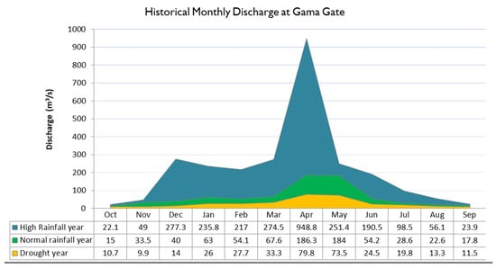
Figure 10.
Historical monthly flow regime (m3/s) at Gama Gate for high, normal and low rainfall years.
3.8.6. Environmental Flows at Gama Gate
The process of obtaining the EFs was carried out as a two-step process:
- The hydraulic engineer obtained the discharge value corresponding to a given water level from a hydrological model set up with the cross-section geometry at Gama Gate. Values for six flow conditions were obtained in the EF workshop.
- These values were extrapolated for other months in accordance with the seasonal pattern present in the historical flow data.
Figure 11 and Figure 12 depict both EFs and historical flows for normal/maintenance years and drought years, respectively, with EFs being lower than historical flows. These EFs are the minimum required flows for a year, or at most, for a couple consecutive years (in case of a prolonged drought). However, whenever possible, flows higher than the EFs should be aimed for, because maintaining flows at EF levels for longer periods (5 years or more) would mean lower than normal flows over the period, thereby stressing the ecosystem. This is because the ecosystem has evolved under historical flow conditions, which, as can be seen in Figure 11 and Figure 12, are greater than the EFs.
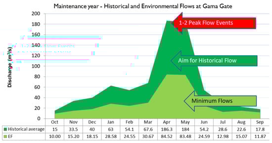
Figure 11.
Recommended minimum freshwater flow (m3/s) guidelines at Gama Gate for a normal rainfall year.
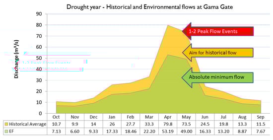
Figure 12.
Minimum recommended freshwater flows (m3/s) at Gama Gate for below-normal (drought) rainfall years.
For a year with normal rainfall (Figure 11—aka “maintenance year”), two data series are shown—the historical monthly flow data (dark green) and the recommended Environmental Flow (light green) that ought to be maintained in the river at Gama for survival of the ecosystem. Note that the recommended flows also follow the seasonal maxima over the March–May high flow period. It is critical to remember that the EFs specifies the minimum flow in the river as measured at Gama to prevent the mortality of large numbers of organisms and ecosystem failure. Hence, water management should strive for flow values higher than the EF, with the EF signifying minimum values to be maintained. On the higher side, the availability of flows higher than EF data series is beneficial, as long as they follow the seasonal historical flow pattern. Indeed, the ecosystem and communities have evolved under the historical average flow conditions—what has been existing in the river, and not under the environmental flows (which is a subset, a guide to ensure critical ecosystem processes are maintained in a particular year). Sudden releases of water, however, are usually detrimental to communities which get washed away; sudden water releases can also erode streambeds.
For drought years i.e., a year with rainfall one standard deviation or lower than the average annual rainfall, a similar EFA visual is shown (Figure 12). The historical monthly flow average is shown in yellow while the minimum recommended EF are in green. Similar to the EF figure for years with normal rainfall (Figure 11), the EF values indicate critical freshwater inflows at Gama gate required to prevent mass aquatic organism mortality due to the river drying up, as well as vastly increasing seawater intrusion. As a rule of thumb, the EF recommendations are targeted towards maintaining the ecosystem in the long term; however, it bears repetition that the local ecosystem has evolved over historically occurring flow conditions, of which the EF is a subset, and any flows greater than the EF are beneficial, as long as they are not an artificial sudden release of water.
Sporadic high flow/flood pulse events: The EFs consider peakflows necessary during the wet season. In addition, very high flows that occur sporadically, such as about once in 5–10 years can be important for the ecosystem. For instance, in the Murray–Darling Basin in Australia, a 1-in-5 year flood event in the Barmah-Millewa Forest was created through releases from a major storage in the Basin, leading to the great egret breeding for the first time since 1979 along with nine species of frogs and native fish [71]. In the Wami Estuary, high flows corresponding to around 10 m. water depth at Gama Gate are thought to be necessary to flush out sediment accumulation and replenish water and nutrients in the oxbow lakes (garuka) which constitute wildlife habitat quite different from the main river channel. However, as that amount would also flood the ranger station, a 7 m water depth once in two years has been recommended. The 1-day flow duration curve for Gama Gate (Figure S1, Supplementary Info) indicates that 100 m3/s of flow occurs or is exceeded 16% of the time in a year. Hence, 2 pulses of 100 m3/s are recommended in addition to the EFs. A flow of 500 m3/s has a return period of about 5 years; hence a flow of 500 m3/s is recommended once in 5 years—typically during a year with high rainfall. Confidence estimates of these recommendations are provided in Supplementary Information.
3.9. EF Comparison with the Montana Method
The EFs decided upon in this study (Figure 11 and Figure 12) are higher than those suggested by the Montana method (Table 7) using the same historical flow dataset. For example, for April–September in a year with normal rainfall (maintenance year—Figure 11), our monthly EF values range from 12–84 m3/s, while the Montana method specifies maintaining at least 25.9 m3/s for a river in good condition. It is to be noted however, that the thresholds in the Montana method (%MAF in Table 7) were specifically developed for trout conservation using a set of 110 temperate western US rivers of similar sizes with similar aquatic ecosystem compositions. Using these thresholds in other parts of the world with very different river flow regimes and ecosystems is not applicable [36], much less for estuaries. Our method developed EFs specifically for the Wami estuary, after evaluating the flow/water depth requirements of plant and animal communities present.
Table 7.
Montana or Tennant Method—Percentage of Mean Annual Flow (%MAF) recommended for different river conditions in two seasons and the corresponding Environmental Flows for maintenance and dry years at Gama Gate. MAF: Mean Annual Flow.
4. Discussion
A dominant concern for Saadani National Park involves diminishing freshwater inflows over time, given increasing anthropogenic multi-sectoral water demand and decreased infiltration/natural water flow regulation resulting from deforestation and wetland drainage across the Wami River basin. Hence, river water management guidelines need to incorporate the natural seasonal variability of water flow and depth in the estuary, as well as directly upstream of Saadani National Park (the section between Gama Gate and Mandera). Such guidelines serve as benchmarks in a programme monitoring freshwater inflow into the downstream estuary.
In the absence of continuous long-term discharge and flow–ecosystem relationship data, the Wami Estuary EFA process relied on a combination of scarce historical data, rapid assessment field data and the judgment of professionals with decades of experience working in Tanzanian and international rivers and estuaries. The fact that the process is carried out as a team effort, in which all experts are together making decisions about sites for study, working side-by-side in the field, and then debating flow recommendations as a group, provides opportunities for team members to learn from each other and examine the results. The involvement of the Tanzanian Ministry of Water and especially the WRBWO was a critical component of the Wami Estuary EFA process, given their leadership role in implementation of the flow recommendations made and their broad knowledge of the Wami Basin’s resources. The Wami Estuary EFA process was directed and carried out entirely by team members who had gained earlier experience from prior EFAs carried out in Tanzania [72,73] and thereby represents the result of capacity building within Tanzania for EFA and the increasing recognition of a team of local experts in ecohydrology, aquatic sciences and their management applications. Below we discuss some points to consider for effective decision-making and implementation of EFs, as well as stress the need for further monitoring to strengthen the confidence in these EFs.
4.1. Environmental Flows: A Subset of Historical Natural Flows
Environmental flows inherently involve a compromise between sustaining the ecosystem and acknowledging the increasing human demand for water. The reality in much of the tropics and subtropics is of diminishing availability of water in rivers caused by increasing water demand, coupled with a loss of the natural ability of catchment ecosystems to maintain seasonal flows on account of the loss of native forests, grasslands and wetlands [74]. Thereby, EF recommendations will usually be less than the historically occurring flows that have influenced the structure and function of local ecosystems.
Plant and animal communities as well as various riverine/riparian ecosystem processes have evolved under seasonally varying water availability, from high flows sweeping off trees and flooding riverbanks to just a trickle at the end of the dry season. Life cycles of various organisms have developed in tune to this seasonal rhythm in flow. As an example, prawns spawn in estuaries during high freshwater inflows, yet conditions in the preceding dry season can affect their fitness which would in turn negatively affect spawning. Apart from seasonal flow changes, there is a considerable amount of inter-annual variation in rainfall and flow as well—years are classified as wet, normal, and dry. Periodic and episodic high flow events are also associated with ecological processes such as fish migration through hydrologically connected floodplains, or the replenishment of nutrients and suppression of invasive vegetation in floodplains, or channel scouring of accumulated sediment and dead vegetation.
Ideally, maintaining the natural seasonal variation in river flow and level that has existed for at least the past several hundred years (free of major human alterations of catchment forest cover and water demands), would ensure ecosystem flow needs. We mention “past several hundred years” as the present-day plant and animal communities have been defined by the hydrological regime with considerable inter-annual variability (more information on this variability is available in a climate study of the Wami Basin [49,75]). However, given the increasing anthropogenic impacts on the catchment, locally and regionally, striving for pre-disturbance era flows is unrealistic. Hence, the team deliberated upon what minimum flows or water depths are necessary for maintaining plant and animal communities along with ecosystem processes such as habitat provision, water quality maintenance, nutrient cycling, and decomposition, to name a few.
It is hence important to realize that Environmental Flows are only a guideline to prevent catastrophic or drastic changes in the ecosystem; however, efforts should be made to provide flows greater than the environmental flows whenever possible. This is usually not an issue in years with high rainfall when plenty of water is available for all uses. The utility of environmental flows guidelines is in years with normal rainfall and is enhanced in years of lower-than-normal rainfall, when water managers must make the increasingly difficult decisions of water allocation between diverse stakeholders.
Freshwater flows to the estuary balance seawater coming in with the tide. Hence, any large decrease in freshwater inflows leads to seawater intrusion into the estuary, and possibly into coastal aquifers near the estuary in areas where the estuary and underlying aquifers are hydrologically connected, or in low-elevation flat areas along riverbanks where seawater floods in overland during low tide. Once shallow well water gets saline, wells often must be abandoned. This is already happening in Bagamoyo district, Tanzania, as evident from coastal village wells that had to be relocated on account of salinization [76]. While coastal salinization is reportedly occurring over a wider section of the coastline in Tanzania, maintaining the seasonal freshwater flows into estuaries can resist the salinization of aquifers in the vicinity of the estuary. Saltwater intrusion has increasingly been occurring in the Pangani estuary over the past several decades [26] and is attributed to two major factors: decreasing freshwater discharge on account of irrigation and hydropower reservoir abstractions and increasing erosion at the marine end on the account of less deposition of river sediment. Despite the importance of estuaries, they remain one of the most negatively impacted ecosystems on the earth mainly due to increasing anthropogenic impacts such as excessive abstraction of water in the catchment, pollution, habitat alterations, eutrophication and overfishing. As a result, the natural functioning of these ecosystems continues to be altered, causing significant impact on productivity and provision of ecosystem services.
4.2. Paucity of Hydrological Data: Monitoring Needs Are Critical
The available streamflow data at the upstream station (Mandera) are not recent, spanning between 1950s to 1980s. There is no reliable information to enable assessment of the present flow situation in most of the stations apart from the few spot discharge measurements. The paucity of hydrologic data at the hydrometric stations in the basin calls for interventions aimed at improving the hydrological monitoring in the catchment. The Gama site is important for the characterization of the inflows into the estuary and hence should be gauged to enable better understanding of the inflows into the estuary. It is also important, underscoring the fact that most of the discharge measurements at Mandera gauging station have been undertaken during the period of low and intermediate flows, thereby missing the high flows. Owing to this, the rating curves better represent low and intermediate flow regimes and cannot be depended on for estimating high flows. Additionally, every high flow has the potential to alter channel geometry by scouring and deposition, thereby necessitating revision of a rating curve developed at a particular place on the river.
It is also beneficial to install and monitor weather stations. The available climatic stations are located upstream in the Wami River basin with very few in the area near the estuary. There are however technical and financial challenges involved in establishing and maintaining a reliable hydrological and climatic monitoring network.
5. Conclusions
The study describes a relatively rapid method to obtain freshwater inflow guidelines for maintaining the existing estuarine ecosystem in a situation where little hydrological data and knowledge of hydrology-ecosystem linkages exists. If basic hydrological data such as mean annual flows exist, other hydrology-based methods such as the Montana method can provide initial environmental flow values, albeit with large uncertainty because these methods do not have a knowledge of local flow-ecosystem links. This knowledge needs to be obtained by fieldwork (as described in this study), that can subsequently be used to customize EF values for a specific estuary.
Even though we mention the essential need for a hydrometric monitoring network, given the swift pace of irreversible ecosystem and environmental degradation resulting from increasing human activity basin wide, waiting to establish such a monitoring network and analyze data obtained therein will take decades and hence be too late. Rapid EFAs as described in this study involving all stakeholders can and should be undertaken to obtain basic quantitative guidelines for water management that can be undertaken within a couple years. These EFs can be changed or fine-tuned in due course with data from a hydrometric monitoring network and longer-scale studies of flow-ecosystem linkages.
Local communities in many parts of the tropics are increasingly aware of the need for coastal wetland restoration to secure mangrove conservation, water quality and sustainable fisheries [4]. Their participation is essential for the success of estuarine ecosystem restoration and sustainable resource use. At the same time, ensuring an adequate freshwater inflow regime requires a basin-wide coordinated approach between water management authorities and other stakeholders in determining a compromise in water allocation for various human and ecosystem needs. As human populations and water needs escalate, coupled with changes in the basin water cycle from land use change and climate change, maintaining adequate freshwater inflows into estuaries becomes ever more critical in order to sustain the varied ecosystem services provided to humanity.
Supplementary Materials
The following supporting information can be downloaded at: https://www.mdpi.com/article/10.3390/hydrology10020033/s1. References citation by [77,78]. Table S1: Physical Description of the EFA sites for hydrological field observations; Table S2: Summary of measured discharges at three locations in August 2015; Table S3: Known water users between Matipwili and Gama Gate (used to estimate water withdrawals and thereby available flows at Gama Gate); Table S4: Summary of maximum flow quantile for the Wami River at Gama; Table S5: Performance of hydraulic model at BBM1 site—Matipwili; Table S6: Performance of hydraulic model at BBM2 site—Gama; Table S7: Global summary statistics of hydraulic model performance and performance rating for both EFA sites; Table S8: Water quality parameters; Table S9: Distance along riverbank occupied by the different plant communities in the Wami River Estuary; Table S10: Fish species encountered in the Wami Estuary Study; Table S11: Estimated population size of terrestrial mammals, their maximum water consumption per day per individual species and per whole population; Table S12: Name, composition and habitat of water birds observed in Wami Estuary; Table S13: Water uses by human communities around the Wami Estuary; Table S14: Maintaining the dry season low flows for drought years (November); Table S15: Maintaining the wet season low flows for drought years (April); Table S16: Maintaining the dry season low flows for maintenance years (October); Table S17: Maintaining the wet season low flows for maintenance years (April); Table S18: Maintaining the wet season high flows for drought years (April); Table S19: Maintaining the wet season high flows for maintenance years (April); Table S20: Confidence levels of the different ecosystem component assessments; Figure S1: Annual Flood Frequency Analysis for Wami River at Gama EFA Site using Log-Pearson Type III (Analysis using Annual Maximum Flow: 1955–1981); Figure S2: Cross-sectional channel profiles of the Wami River ar BBM1-Matipwili; Figure S3: Channel cross-sectional profile of the Wami River at BBM2-Gama; Figure S4: Flow speed and water depth at Gama Gate; Figure S5: Wami Estuary Channel bathymetry upto freshwater vegetation section; Figure S6: Water clarity during ebb (20 -Aug-15) and flood (24- Aug-15) tides; Figure S7: Catch composition of fish species at different locations in the Wami River estuary and within 2 km offshore (Chanyungu). Numbers indicate number of individual fish species caught; Figure S8: Number of fish caught in one day (August 2015) by fishermen at Kanjanjo and Saadan village landing sites; Figure S9: Number of hippos (left) and primates (right) in different habitats. Errata: left graph should read 59, 51, 4 and 39 individuals of hippopotami; Figure S10: Water required per population of terrestrial wildlife species in Sadaani National Park; Figure S11: Number of individuals and number of bird species encountered in different habitat types.
Author Contributions
Conceptualization, A.K.S. and M.C.D.; methodology, A.K.S., J.K., F.M., R.T., H.K., M.K., P.H., P.M., M.M.I., T.M., R.E., R.M. and I.O.; formal analysis, A.K.S., J.K., F.M., M.K. and P.M.; investigation, all authors except M.C.D.; resources, M.C.D.; data curation, A.K.S., H.K., J.K., F.M., P.M. and M.K.; writing—original draft preparation, A.K.S., J.K., F.M., P.M., M.M.I., M.K. and P.H.; writing—review and editing, A.K.S. and M.K.; visualization, A.K.S., J.K. and F.M.; supervision, A.K.S.; project administration, A.K.S., M.A.M. and M.C.D.; funding acquisition, M.C.D. All authors have read and agreed to the published version of the manuscript.
Funding
The study was funded by the American people through the U.S. Agency for International Development (USAID).
Data Availability Statement
Please refer to suggested Data Availability Statements in section “MDPI Research Data Policies” at https://www.mdpi.com/ethics (accessed on: 14 January 2023).
Acknowledgments
This study was facilitated by Praxeda Kalugendo, the Basin Water Officer, Wami Ruvu Basin Water Office and Juliana Msaghaa, District Water Officer, Bagamoyo. Hydrology technicians Elbariki Daudi, Joseph Twiga (WRBWO) and Samson (University of Dar es Salaam) assisted in data collection and surveying. The staff of Saadani National Park—Hassan Mohamed Nguluma (Chief Park Warden), Rukia Malya, Angela Solomon and Sharif Hassan were very cooperative and eased the way for fieldwork across eight months in a very challenging terrain. Special thanks to Camp Manager Kanji (late) for all his immense help at Kinyonga Camp, Saadani National Park. Vivienne Abbott and Maria C. Donoso of the USAID-supported IWASH program were instrumental in bringing this study to fruition. Elizabeth Anderson from FIU, who had prior experience with aquatic ecology and environmental flows in East Africa helped shape the study with her suggestions. Leodgard Haule of IWASH Tanzania greatly helped in organizing the human dimensions component of the study from his vast experience with community engagement in Tanzania. Lastly, we are thankful to the handling editor and three anonymous reviewers whose comments and suggestions greatly improved the clarity and scientific rigor of the manuscript.
Conflicts of Interest
The funders had no role in the design of the study; in the collection, analyses, or interpretation of data; in the writing of the manuscript, or in the decision to publish the results.
References
- Pritchard, D.W. What is an estuary: Physical viewpoint. In Estuaries; Lauf, G.H., Ed.; American Association for the Advancement of Science: Washington, DC, USA, 1967; Volume 1, pp. 149–176. [Google Scholar]
- Uncles, R.; Stephens, J.; Smith, R. The dependence of estuarine turbidity on tidal intrusion length, tidal range and residence time. Cont. Shelf Res. 2002, 22, 1835–1856. [Google Scholar] [CrossRef]
- Barbier, E.B.; Hacker, S.D.; Kennedy, C.; Koch, E.W.; Stier, A.C.; Silliman, B.R. The value of estuarine and coastal ecosystem services. Ecol. Monogr. 2011, 81, 169–193. [Google Scholar] [CrossRef]
- Sinclair, M.; Sagar, M.K.V.; Knudsen, C.; Sabu, J.; Ghermandi, A. Economic appraisal of ecosystem services and restoration scenarios in a tropical coastal Ramsar wetland in India. Ecosyst. Serv. 2021, 47, 101236. [Google Scholar] [CrossRef]
- Wolanski, E.; Boorman, L.A.; Langlois-Saliou, E.; Lara, R.; Plater, A.J.; Uncles, R.J.; Zalewski, M. Ecohydrology as a new tool for sustainable management of estuaries and coastal waters. Wetl. Ecol. Manag. 2004, 12, 235–276. [Google Scholar] [CrossRef]
- Semesi, A.K. Developing management plans for the mangrove forest reserves of mainland Tanzania. In The Ecology of Mangrove and Related Ecosystems; Springer: Dordrecht, The Netherlands, 1992; pp. 1–10. [Google Scholar]
- Bwathondi, P.O.J.; Mwamsojo, G.O.J. The status of the fishery resource in, the wetlands of Tanzania. In Wetlands of Tanzania, Proceedings of a Seminar on Wetlands of Tanzania, Morogoro 27–29 November 1991; Kamukala, G.L., Crafter, S.A., Eds.; Tanzania Fisheries Research Institute 1993; 170p, Available online: https://aquadocs.org/handle/1834/525 (accessed on 14 January 2023).
- Nagelkerken, I.; Kleijnen, S.; Klop, T.; Van Den Brand, R.A.; de La Moriniere, E.C.; Van der Velde, G. Dependence of Caribbean reef fishes on mangroves and seagrass beds as nursery habitats: A comparison of fish faunas between bays with and without mangroves/seagrass beds. Mar. Ecol. Prog. Ser. 2001, 214, 225–235. [Google Scholar] [CrossRef]
- Sheaves, M. Consequences of ecological connectivity: The coastal ecosystem mosaic. Mar. Ecol. Prog. Ser. 2009, 391, 107–115. [Google Scholar] [CrossRef]
- Igulu, M.M.; Nagelkerken, I.; van der Velde, G.; Mgaya, Y.D. Mangrove Fish Production is Largely Fuelled by External Food Sources: A Stable Isotope Analysis of Fishes at the Individual, Species, and Community Levels from Across the Globe. Ecosystems 2013, 16, 1336–1352. [Google Scholar] [CrossRef]
- Martin, E.B.; Martin, C.P. Cargoes of the East: The Ports, Trade and Culture of the Arabian Seas and Western Indian Ocean; Elm Tree Books: London, UK, 1978; p. 244. ISBN 0241898552. [Google Scholar]
- Semesi, A.K.; Msumi, G.D.; Kivia, D.; Lilungulu, J.; Magege, D.; Mgaya, Y.D.; Kalangahe, B.; Muruke, M.; Kuguru, B.; Francis, J.; et al. Coastal resources of Bagamoyo District, Tanzania. Conference on Advances on Marine Sciences in Tanzania. 2000. Available online: https://www.sciencebase.gov/catalog/item/50540367e4b097cd4fcfac9b (accessed on 14 January 2023).
- Goldberg, L.; Lagomasino, D.; Thomas, N.; Fatoyinbo, T. Global declines in human-driven mangrove loss. Glob. Chang. Biol. 2020, 26, 5844–5855. [Google Scholar] [CrossRef]
- Drinkwater, K.F.; Frank, K.T. Effects of river regulation and diversion on marine fish and invertebrates. Aquat. Conserv. Mar. Freshw. Ecosyst. 1994, 4, 135–151. [Google Scholar] [CrossRef]
- Sklar, F.H.; Browder, J.A. Coastal Environmental Impacts Brought About by Alterations to Freshwater Flow in the Gulf of Mexico. Environ. Manag. 1998, 22, 547–562. [Google Scholar] [CrossRef]
- Alber, M. A conceptual model of estuarine freshwater inflow management. Estuaries 2002, 25, 1246–1261. [Google Scholar] [CrossRef]
- Powell, G.L.; Matsumoto, J.; Brock, D.A. Methods for determining minimum freshwater inflow needs of Texas bays and estuaries. Estuaries 2002, 25, 1262–1274. [Google Scholar] [CrossRef]
- Estevez, E.D. Review and assessment of biotic variables and analytical methods used in estuarine inflow studies. Estuaries 2002, 25, 1291–1303. [Google Scholar] [CrossRef]
- Arthington, A.H.; Finlayson, C.M.; Roux, D.J.; Nel, J.L.; Rast, W.; Froend, R.; Turpie, J.; van Niekerk, L. Managing specific freshwater ecosystems. In Freshwater Ecosystems in Protected Areas; Routledge: London, UK, 2018; pp. 144–176. ISBN 9781315226385. [Google Scholar]
- Pringle, C.M. Hydrologic connectivity and the management of biological reserves: A global perspective. Ecol. Appl. 2001, 11, 981–998. [Google Scholar] [CrossRef]
- Layman, C.A.; Allgeier, J.E.; Rosemond, A.D.; Dahlgren, C.P.; Yeager, L.A. Marine fisheries declines viewed upside down: Human impacts on consumer-driven nutrient recycling. Ecol. Appl. 2011, 21, 343–349. [Google Scholar] [CrossRef] [PubMed]
- Fourqurean, J.W.; Boyer, J.N.; Durako, M.J.; Hefty, L.N.; Peterson, B.J. Forecasting Responses of Seagrass Distributions to Changing Water Quality Using Monitoring Data. Ecol. Appl. 2003, 13, 474–489. [Google Scholar] [CrossRef]
- Barletta, M.; Barletta-Bergan, A.; Saint-Paul, U.; Hubold, G. The role of salinity in structuring the fish assemblages in a tropical estuary. J. Fish Biol. 2005, 66, 45–72. [Google Scholar] [CrossRef]
- Nguyen, A.D.; Savenije, H.H. Salt intrusion in multi-channel estuaries. Hydrol. Earth Syst. Sci. 2006, 10, 743–754. [Google Scholar] [CrossRef]
- Parida, A.K.; Das, A.B. Salt tolerance and salinity effects on plants: A review. Ecotoxicol. Environ. Saf. 2005, 60, 324–349. [Google Scholar] [CrossRef]
- Sotthewes, W. Forcing on the Salinity Distribution in the Pangani Estuary. Master’s Thesis, University of Delft, Delft, The Netherlands, 2008; p. 82. [Google Scholar]
- Tolley, S.G.; Brosious, B.B.; Peebles, E.B. Recruitment of the Crabs Eurypanopeus depressus, Rhithropanopeus harrisii, and Petrolisthes armatus to Oyster Reefs: The Influence of Freshwater Inflow. Estuaries Coasts 2013, 36, 820–833. [Google Scholar] [CrossRef]
- Arthington, A.H.; Bhaduri, A.; Bunn, S.E.; Jackson, S.E.; Tharme, R.E.; Tickner, D.; Young, B.; Acreman, M.; Baker, N.; Capon, S.; et al. The Brisbane Declaration and Global Action Agenda on Environmental Flows (2018). Front. Environ. Sci. 2018, 6, 45. [Google Scholar] [CrossRef]
- Schlacher, T.A.; Wooldridge, T.H. Ecological responses to reductions in freshwater supply and quality in South Africa’s estuaries: Lessons for management and conservation. J. Coast. Conserv. 1996, 2, 115–130. [Google Scholar] [CrossRef]
- Benson, N.G. The freshwater-inflow-to-estuaries issue. Fisheries 1981, 6, 8–10. [Google Scholar] [CrossRef]
- Knowles, N. Natural and management influences on freshwater inflows and salinity in the San Francisco Estuary at monthly to interannual scales. Water Resour. Res. 2002, 38, 25-1. [Google Scholar] [CrossRef]
- Arthington, A.H.; Tharme, R.E.; Brizga, S.O.; Pusey, B.J.; Kennard, M.J. Environmental Flow Assessment with emphasis on holistic methodologies. In Proceedings of the Second International Symposium on the Management of Large Rivers for Fisheries, Phnom Penh, Cambodia, 11–14 February 2003; Welcomme, R., Petr, T., Eds.; FAO Regional Office for Asia and the Pacific: Bangkok, Thailand, 2004. Available online: http://www.fao.org/docrep/007/ad526e/ad526e07.htm#bm07 (accessed on 14 January 2023).
- Sun, T.; Yang, Z.; Shen, Z.; Zhao, R. Environmental flows for the Yangtze Estuary based on salinity objectives. Commun. Nonlinear Sci. Numer. Simul. 2009, 14, 959–971. [Google Scholar] [CrossRef]
- Adams, J.B.; Cowie, M.; Van Niekerk, L. Assessment of Completed Ecological Water Requirement Studies for South African Estuaries and Responses to Changes in Freshwater Inflow; Water Research Commission: Pretoria, South Africa, 2016; pp. 1–57. [Google Scholar]
- Tennant, D.L. Instream Flow Regimens for Fish, Wildlife, Recreation and Related Environmental Resources. Fisheries 1976, 1, 6–10. [Google Scholar] [CrossRef]
- Kawde, S.K.; Jain, M.K.; Durbude, D.G. Environmental Flows Assessment: A Review. J. Indian Water Resour. Soc. 2016, 36. [Google Scholar]
- Smakhtin, V.U.; Piyankarage, S.C.; Stanzel, P.; Boelee, E. Simulating the Hydrology of Small Coastal Ecosystems in Conditions of Limited Data; Research Report 77; International Water Management Institute (IWMI): Colombo, Sri Lanka, 2004. [Google Scholar]
- Karimi, S.S.; Yasi, M.; Eslamian, S. Use of hydrological methods for assessment of environmental flow in a river reach. Int. J. Environ. Sci. Technol. 2012, 9, 549–558. [Google Scholar] [CrossRef]
- Alfieri, L.; Bisselink, B.; Dottori, F.; Naumann, G.; de Roo, A.; Salamon, P.; Wyser, K.; Feyen, L. Global projections of river flood risk in a warmer world. Earth’s Futur. 2017, 5, 171–182. [Google Scholar] [CrossRef]
- Poff, N.L.; Tharme, R.E.; Arthington, A.H. Evolution of Environmental Flows Assessment Science, Principles, and Methodologies. In Water for the Environment; Elsevier: Amsterdam, The Netherlands, 2017; pp. 203–236. [Google Scholar] [CrossRef]
- Pielou, E.C. Freshwater. University of Chicago Press: Chicago. IL, USA, 1998; 275p, ISBN 9780226668161. [Google Scholar]
- Kiwango, H.; Njau, K.N.; Wolanski, E. The need to enforce minimum environmental flow requirements in Tanzania to preserve estuaries: Case study of mangrove-fringed Wami River estuary. Ecohydrol. Hydrobiol. 2015, 15, 171–181. [Google Scholar] [CrossRef]
- Burgess, N.D.; Abdallah, J.; Lukumbuzya, K.; Urock, J.; Malugu, I.; Sumbi, P.; Kijazi, A.; Milledge, S.; Schaafsma, M.; Makala, J. Trends in the production of charcoal and timber from Tanzania’s Coastal Forests. Arc J. Tanzan. For. Conserv. Group Biannu. Newsl. 2013, 28, 25–30. [Google Scholar]
- Mligo, C. Diversity and distribution pattern of riparian plant species in the Wami River system, Tanzania. J. Plant Ecol. 2016, 10, 259–270. [Google Scholar] [CrossRef]
- Anderson, E.; McNally, C. A Rapid Environmental Assessment of the Wami River Estuary, Tanzania 2008. Available online: http://www.ci.uri.edu/ciip/Publications/McNally_WamiEstuary_RapidEcologicalAssessment.pdf (accessed on 14 January 2023).
- IUCN Eastern and Southern Africa Programme. The Wami Basin: A Situation Analysis. 2010. Available online: https://portals.iucn.org/library/node/9604?cookies-complaint=1 (accessed on 14 January 2023).
- WRWBO. Annual Hydrological Report 2009/2010; Wami Ruvu Basin Water Office: Morogoro, Tanzania, 2010; p. 43.
- Valimba, P. Environmental Flow Assessment (EFA), Wami River Sub-Basin, Tanzania: Hydrology Component of the Wami River EFA Study; Literature Review for BBM Workshop; Wami-Ruvu Basin Water Office: Morogoro, Tanzania, 2007; 33p.
- Saha, A.; Donoso, M.; Mohamed, A.; Masikini, R.; Abbott, V.; Anderson, E. Water Atlas of the Wami Ruvu Basin, Tanzania. In Global Water for Sustainability Program; Florida International University: Miami, FL, USA, 2014; 105p, ISBN 978-1-941993-01-9. [Google Scholar]
- Castellarin, A.; Camorani, G.; Brath, A. Predicting annual and long-term flow-duration curves in ungauged basins. Adv. Water Resour. 2007, 30, 937–953. [Google Scholar] [CrossRef]
- Yokoo, Y.; Sivapalan, M. Towards reconstruction of the flow duration curve: Development of a conceptual framework with a physical basis. Hydrol. Earth Syst. Sci. 2011, 15, 2805–2819. [Google Scholar] [CrossRef]
- Chow, V.T. Open-Channel Hydraulics; McGraw-Hill: New York, NY, USA, 1959; 680p. [Google Scholar]
- Tharme, R.E.; King, J.M. Development of the Building Block Methodology for Instream Flow Assessments and Supporting Research on the Effects of Different Magnitude Flows on Riverine Ecosystems; Water Research Commission Report No. 576/1/98; Water Research Commission: Pretoria, South Africa, 1998; 452 p. [Google Scholar]
- Acreman, M.C.; Dunbar, M.J. Defining environmental river flow requirements—A review. Hydrol. Earth Syst. Sci. 2004, 8, 861–876. [Google Scholar] [CrossRef]
- King, J.M.; Tharme, R.E.; Villiers, M.S. Environmental Flow Assessment For Rivers: Manual For the Building Block Methodology; Water Research Commision (WRC) Report No: TT 131/00; Water Research Commission: Pretoria, South Africa, 2000; ISBN 1 86845 628 5. [Google Scholar]
- Semesi, A.K. Mangrove management and utilization in Eastern Africa. Ambio 1998, 27, 620–626. [Google Scholar]
- Richmond, M.D. (Ed.) A Field Guide To the Seashores of Eastern Africa and the Western Indian Ocean Islands; Sida/WIOMSA – Western Indian Ocean Marine Science Association: Zanzibar, Tanzania, 2011; 464p, ISBN 99867-8977-9-7. [Google Scholar]
- Saha, A.K.; Saha, S.; Sadle, J.; Jiang, J.; Ross, M.S.; Price, R.M.; Sternberg, L.S.L.O.; Wendelberger, K.S. Sea level rise and South Florida coastal forests. Clim. Chang. 2011, 107, 81–108. [Google Scholar] [CrossRef]
- Mligo, C.; Lyaruu, H.; Ndangalasi, H.; Marchant, R. Vegetation Community Structure, Composition and Distribution Pattern in the Zaraninge Forest, Bagamoyo District, Tanzania. J. East Afr. Nat. Hist. 2009, 98, 223–239. [Google Scholar] [CrossRef]
- Silas, M.O. Review of the Tanzanian Prawn Fishery. Master’s Thesis, Department of Biology, University of Bergen, Bergen, Norway, 2011. Available online: https://bora.uib.no/bora-xmlui/handle/1956/5584 (accessed on 14 January 2023).
- Tumbo, M.; Mangora, M.M.; Pauline, N.M.; Kuguru, B. Review of Literature for a Climate Vulnerability Assessment in the RUMAKI Seascape, Tanzania; Report for WWF Tanzania, Dar es Salaam, Tanzania. 2015. Available online: https://www.academia.edu/12695184/Review_of_Literature_for_a_Climate_Vulnerability_Assessment_in_the_RUMAKI_Seascape_Tanzania (accessed on 14 January 2023).
- Mosha, E.J.; Gallardo, W.G. Distribution and size composition of penaeid prawns, Penaeus monodon and Penaeus indicus in Saadani estuarine area, Tanzania. Ocean Coast. Manag. 2013, 82, 51–63. [Google Scholar] [CrossRef]
- Tamatamah, R.A. Environmental Flow Assessment (EFA), Wami River Sub-Basin, Tanzania: Aquatic Ecology Component of the Wami River EFA Study; Literature Review for BBM Workshop; Wami-Ruvu Basin Water Office: Morogoro, Tanzania, 2007; 26p.
- West, G.; Heard, D.; Caulkett, N. Zoo Animal and Wildlife Immobilization and Anesthesia, 2nd ed.; John Wiley & Sons: Hoboken, NJ, USA, 2014; p. 976. ISBN 978-0-813-81183-3. [Google Scholar] [CrossRef]
- DE Magalhães, J.P.; Costa, J. A database of vertebrate longevity records and their relation to other life-history traits. J. Evol. Biol. 2009, 22, 1770–1774. [Google Scholar] [CrossRef]
- Lewison, R. Population responses to natural and human-mediated disturbances: Assessing the vulnerability of the common hippopotamus (Hippopotamus amphibius). Afr. J. Ecol. 2007, 45, 407–415. [Google Scholar] [CrossRef]
- Lewison, R.; Oliver, W. Hippopotamus Amphibius. IUCN Red List of Threatened Species. 2008. Available online: http://www.iucnredlist.org/apps/redlist/details/10103/0 (accessed on 14 January 2023).
- Estes, R. The Behavior Guide to African Mammals: Including Hoofed Mammals, Carnivores, Primates; Unversity of California Press: Los Angeles, CA, USA, 1992. [Google Scholar]
- Roomer, A. Anecdotal and Descriptive Natural History: The Hippopotamus; Groombridge: London, UK, 1872. [Google Scholar]
- Stevenson-Hamilton, J. Animal Life in Africa; E.P. Dutton and Company: New York, NY, USA, 1912. [Google Scholar]
- Dyson, M.; Bergkamp, G.; Scanlon, J. (Eds.) Flow: The Essentials of Environmental Flows; IUCN: Gland, Switzerland; Cambridge, UK, 2003; 118p. [Google Scholar]
- FIU-GLOWS 2014 a; A Rapid Ecohydrological Assessment of the Ruvu River Estuary, Tanzania. Global Water for Sustainability Program. Florida International University: Miami, FL, USA, 2014; 77p.
- FIU-GLOWS 2014, b; Ruvu River Basin, Tanzania: Environmental Flow Assessment. Global Water for Sustainability Program, Florida International University: Miami, FL, USA, 2014; 76p.
- Seeteram, N.A.; Hyera, P.T.; Kaaya, L.T.; Lalika, M.C.; Anderson, E.P. Conserving rivers and their biodiversity in Tanzania. Water 2019, 11, 2612. [Google Scholar] [CrossRef]
- FIU-GLOWS 2014, c; Climate and Landscape-Related Vulnerability of Water Resources in the Wami/Ruvu River Basin, Tanzania. In Global Water for Sustainability Program. Florida International University: Miami, FL, USA, 2014; 110p.
- Tobey, J. A profile of the Wami River Sub-basin. Report prepared for USAID by the Tanzania Coastal Management Program and the Coastal Resources Center; University of Rhode Island: Providence, RI, USA, 2008; 21p. [Google Scholar]
- Gritzner, J.; Jemison, R. USDA Forest Service Technical Assistance Trip Report. Available online: https://www.crc.uri.edu/download/USFS_Wami_Wetlands_Gritzner_Jemison_2009.pdf (accessed on 21 November 2022).
- McNally, C. A Follow-Up Dry Season Rapid Ecological Assessment of the Wami River Estuary, Tanzania; Coastal Resources Center, University of Rhode Island: Kingston, RI, USA, 2007. Available online: https://pdf.usaid.gov/pdf_docs/PNADN808.pdf (accessed on 21 November 2022).
Disclaimer/Publisher’s Note: The statements, opinions and data contained in all publications are solely those of the individual author(s) and contributor(s) and not of MDPI and/or the editor(s). MDPI and/or the editor(s) disclaim responsibility for any injury to people or property resulting from any ideas, methods, instructions or products referred to in the content. |
© 2023 by the authors. Licensee MDPI, Basel, Switzerland. This article is an open access article distributed under the terms and conditions of the Creative Commons Attribution (CC BY) license (https://creativecommons.org/licenses/by/4.0/).