1. Introduction
Hydrodynamic models are indispensable tools used to simulate the movement of water in different types of water bodies, and for various purposes. In oceans, hydrodynamic models can be used to help characterize the tides [
1] and to simulate regional oceanic circulation [
2]. In estuaries, hydrodynamic model results can be used to simulate shallow water wave motions [
3,
4], to simulate flooding [
5], as input to water quality models, for purposes including water project operation [
6], and as input to particle tracking models [
7], for purposes including determining the effects of water project operations on fish survival rates [
8,
9,
10]. In riverine systems, hydrodynamic modeling can be used to better understand flood risks [
11] and to evaluate the effects of dredging [
12].
Hydrodynamic models require an understanding of the shapes of the beds of river channels and other waterbodies in the systems they simulate. Geometry input datasets, created using bathymetry data, describe these shapes to the models. The geometry data requirements of a model depend in part upon its dimensionality. Hydrodynamic model dimensionality can be one-dimensional (1D) (DSM2 [
13,
14] and HEC-RAS [
15]), two-dimensional (2D) (RMA2 [
16,
17], HEC-RAS [
15]), or three-dimensional (3D) (Delft 3D [
18], SCHISM [
19,
20], SUNTANS [
21,
22], UnTRIM [
23,
24].
Multidimensional model geometry creation requires a continuous surface created from channel bathymetry data. Examples are a Digital Elevation Model (DEM) or Digital Terrain Model (DTM), such as a river terrain model [
25]. Both types of surfaces can be created from datasets such as bathymetry data and cross-sections. Surfaces can be further refined using tools such as the GIS-based tool Waterscape Subbasin Identification (WASUBI), which identifies subbasins [
26]. Tools used to create geometry for 1D models can also use a continuous surface, but they generally do not require it, since they can also work with bathymetry point data.
Three-dimensional model geometry, also known as a mesh, consists of 3D polygonal elements, which have a node at each vertex of the elements. Mesh development software displays a mesh as a set of points connected by lines. Each node has x, y, and z coordinates, which determine the shapes and sizes of the elements. A mesh can be structured or un-structured. An unstructured mesh allows grid size and shape to vary as needed to ap-propriate size for the resolution needed, given the variations in the bottom contours. Different 3D models have different constraints on element shape [
27]. Tools to create 3D meshes include Aquaveo SMS, used for SCHISM and other multidimensional models, and RiverBox [
28], which is an ArcGIS toolbox. Two-dimensional model geometry input is similar to a 3D model geometry input, consisting of a mesh of 2D polygons. The mesh is visualized as a flat surface, but each node has an elevation defined, which is typically determined using a continuous surface created from bathymetry data. HEC-RAS and RMA2 both can include 2D elements in their meshes, as well as 1D elements. Tools to create 2D meshes include Aquaveo SMS and the HEC-RAS 2D Flow Area editor [
15].
Cross-sections for 1D models are created exactly or approximately perpendicular to the channel center lines of a river system. The shapes of the cross-sections are derived from bathymetry data, either as individual points, or as a surface created using GIS, such as a DEM. Coordinate systems are channel-based, with cross-section point coordinates measured in the longitudinal and transverse directions. Cross-sections are placed as needed to approximate the variations in the channel bathymetry that are most important for the accuracy of the flow simulation. Examples of 1D models using this approach include DSM2 [
14] and HEC-RAS [
15]. Tools used to create cross-sections for 1D models include HEC-RAS, the Advanced Spaceborne Thermal Emission and Reflection (ASTER) Radiometer Global Digital Elevation Model [
29], and RiverBox [
28]. HEC-RAS (USACE), ASTER [
29], and RiverBox [
28] all have the option to create cross-sections automatically, using DEM data. ASTER also has the ability to create synthetic cross-sections using a rating curve derived from observed data. Automatic cross-section creation may be less time-consuming than manual cross-section creation, but it requires a surface such as a DEM, created from high-quality bathymetry data, and in the case of ASTER, the automatically created cross-sections must be adjusted manually to exclude lower-quality data [
29]. ASTER’s method of creating synthetic cross-sections appears to be useful in areas lacking adequate bathymetry data, but their applicability of these cross-sections outside the range of hydrologic conditions used to develop them is not discussed [
29]. HEC-RAS, in addition to creating cross-sections automatically, allows the user to create and edit cross-sections manually by entering and/or modifying station and elevation coordinates for each cross-section [
15]. RiverBox is a tool for creating cross-sections automatically, using interpolation to create reasonable approximations in areas with relatively sparse bathymetry [
28]. The method used by RiverBox is almost completely automated, and it appears to assume that all bathymetry data are of equal quality.
Automated approaches to cross-section creation can save time and yield more consistent results. However, they either assume that all data used to create them are of equal quality, or they include a method for making manual adjustments to cross-sections. The current study proposes a parsimonious cross-section development tool: the Cross-Section Development Program (CSDP). It is an open-source application written in Java. It is a standalone application, requiring no other software, such as GIS. It is easy to use, and is designed specifically to create input for DSM2 [
14] but also can be applied to other hydrodynamic models. The CSDP differs from the other tools described above in that the placement of channel centerlines, cross-section lines, and cross-section points are all conducted manually. This has the advantage of allowing the user full control over cross-section creation, allowing the user to place more emphasis on bathymetry data considered to be higher quality, and to easily incorporate proposed changes to channels, such as dredging. However, the manual cross-section development process can be time consuming, and results for a given set of input data will be more variable than results from automated tools.
The process of creating cross-sections with the CSDP involves clicking on a graph of bathymetry data and/or DEM data. The bathymetry points on the graph can be color-coded to identify attributes such as collection year or data source. The use of a DEM requires more pre-processing of bathymetry data, and can make variations in data quality less obvious to the user. The CSDP also includes a tool to display bathymetry data together with cross-sections in a 3D interactive plot [
30], allowing the user to zoom, pan, and rotate the plot to determine qualitatively how the cross-sections compare to the bathymetry data. The 3D plot can also help the user identify features that the user may wish to exclude from model geometry, such as narrow deep holes.
This paper describes the application of the CSDP for developing geometry for DSM2, including descriptions of bathymetry data used by the CSDP, the DSM2 model grid, and DSM2 geometry input requirements. The usage of the CSDP graphical user interface (GUI) is then demonstrated, including creating channel centerlines, cross-section lines, and cross-sections. Recently added CSDP features for adjusting cross-sections to match bathymetry data are introduced, along with best practices for cross-section development, and adjusting cross-sections to match channel volumes calculated using GIS. The results of a recent DSM2 calibration using geometry updated with the CSDP are then presented.
3. The Cross-Section Development Program
This section presents the purpose and scope of the Cross-Section Development Program (CSDP), the graphic user interface (GUI) of the CSDP, and some of the CSDP main features. CSDP software availability is detailed in
Appendix A. A nomenclature summarizing abbreviations used in this paper is provided in
Appendix B.
3.1. Purpose and Scope of the CSDP
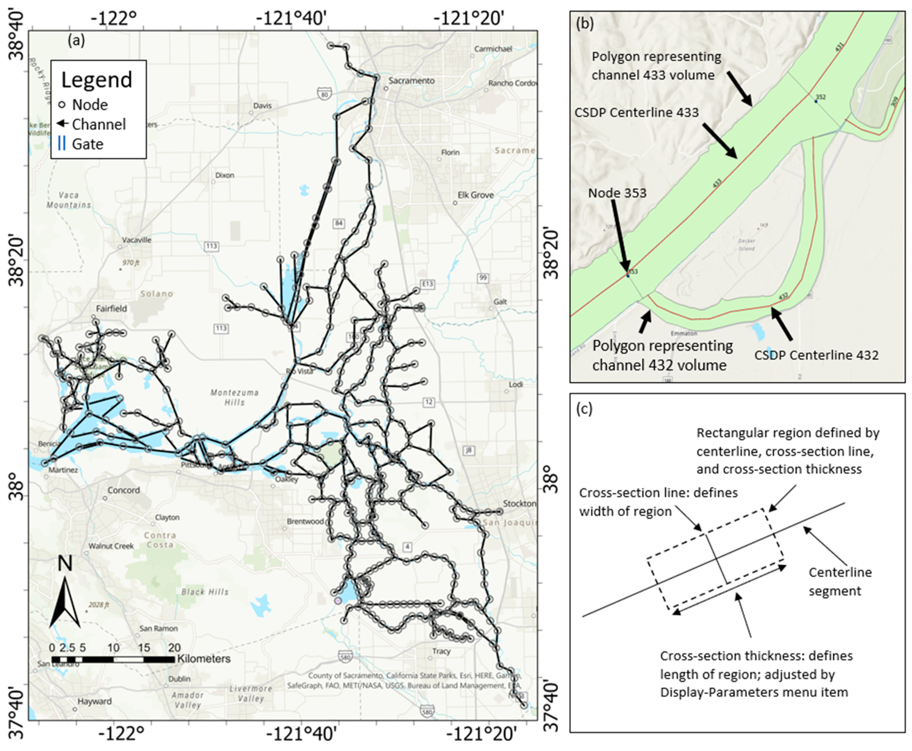
The CSDP is designed to create geometry inputs for hydrodynamic models. These inputs include a geo-referenced grid network of channels, nodes, reservoirs, and flow and water quality control facilities (e.g., gates) representing the real-world modeling domain (e.g.,
Figure 1a), cross-sections approximating the shape of each channel, and conveyance characteristics of each cross-section.
In hydrodynamic models, each channel is typically connected to other channels by nodes located at channel endpoints. The CSDP uses channel centerlines to represent channels (e.g.,
Figure 1b). The CSDP uses landmarks to represent features whose location can be described using a single set of geographic coordinates. Landmarks appear as points with text labels in the CSDP and are used to represent nodes and other features. Each channel can be divided to several polygonal regions, which are defined by the centerline, cross-section line, and cross-section thickness (
Figure 1c). Each channel can have one or more cross-sections. Each cross-section’s location is defined by channel number and the distance measured along the channel centerline from the upstream end toward the downstream end. Cross-section lines are always perpendicular to the centerline segment that they intersect. A cross-section represents a portion of the channel that extends either all the way to the node or half the distance to adjacent cross-sections. Ideally, the cross-section thickness should be sufficiently large to include the entire portion of the channel that it represents, but in practice, the thickness is often reduced depending mostly upon the curvature of the channel and the density of the bathymetry data. In the CSDP, the channel centerlines, cross-section lines, and cross-section drawings are referred to as the “network”.
The CSDP calculates the following conveyance characteristics for each cross-section: area, width, wetted perimeter, hydraulic radius, x centroid, and z centroid. Based on these metrics, the channel volume can be derived. The CSDP’s functionality for viewing and calculating cross-sections can also be used to analyze bathymetry data for use in developing model inputs for reservoirs and gates that represent weirs.
3.2. The CSDP GUI
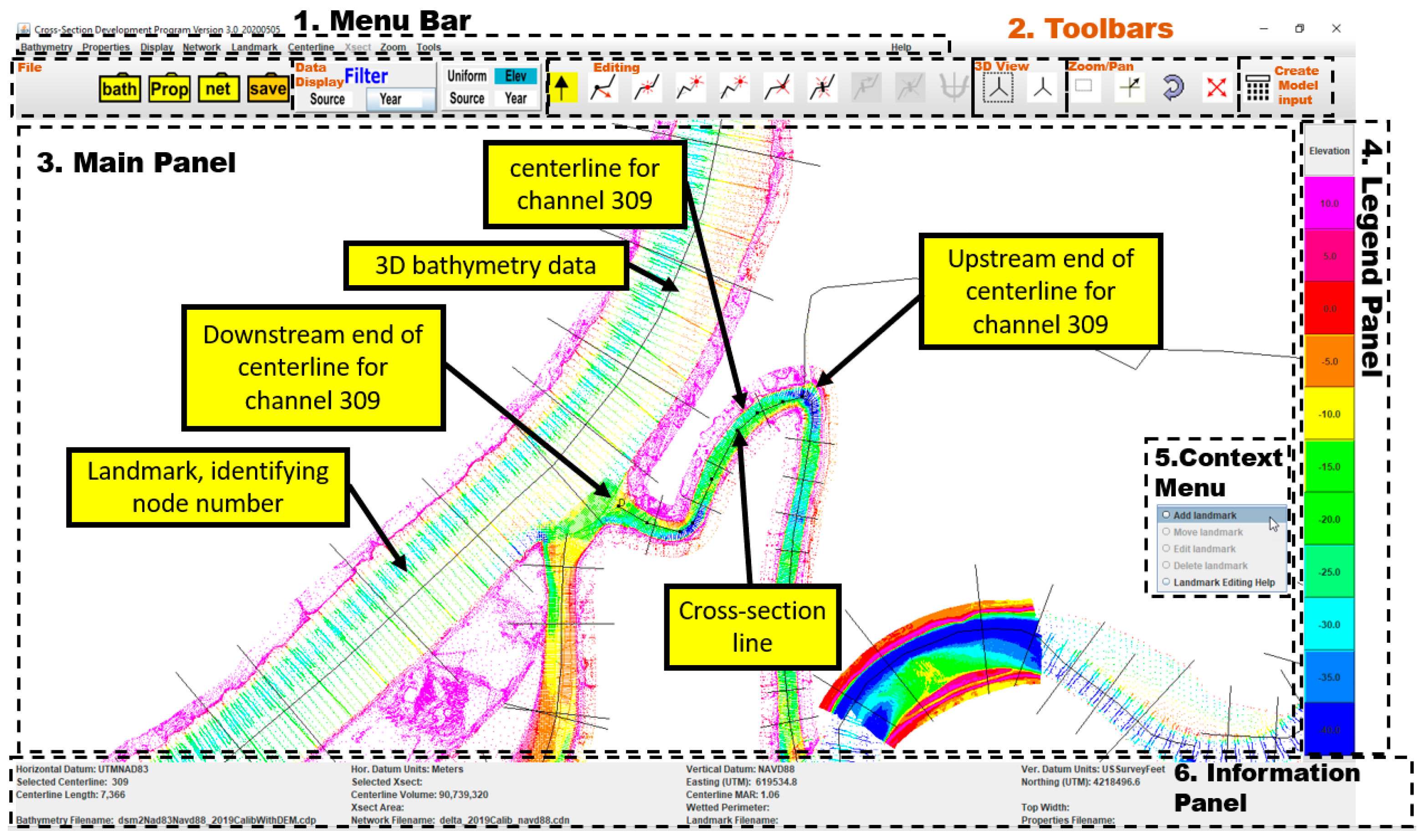
The main application window of the CSDP contains six main components: a menu bar, a set of toolbars, a main panel, a legend panel, an information panel, and a context menu for creating and editing landmarks (
Figure 2). The menu bar includes ten menus, which provide access to most of the CSDP functionality. The “bathymetry” menu is for loading and saving bathymetry data files. The “properties” menu is for loading and saving files that contain various program options. The “display” menu is for adjusting program options, filtering the display of bathymetry data, changing the bathymetry data color scheme, and loading a file that displays channel outlines. The “network” menu is for loading and saving network (channels and cross-section) files, creating various types of bathymetry plots and network diagnostics, and creating DSM2 geometry input. The “landmark” menu is for loading and saving landmark (locations of nodes or other features) files. The “centerline” menu is for editing channel centerlines and cross-section lines, and for creating various types of bathymetry and cross-section plots. The “Xsect” menu is for viewing and editing cross-sections.
Section 3.3 discusses cross-section editing in detail. The “zoom” menu is for zooming and panning the bathymetry display in the main panel. The “tools” menu is for accessing a number of functions for viewing and manipulating CSDP data. The “help” menu displays the CSDP license information.
The main function of the toolbars is to provide easy access to the most commonly used functions that are also accessible through the menu bar. The file toolbar is for loading bathymetry, properties, and network files, and for saving the currently loaded network file. The data display toolbar includes a filter panel and a color scheme panel. The data display filter panel (on the left) is for toggling the display of bathymetry data for selected sources (data provider names) and/or years. The data display color scheme panel (on the right) is for setting the color scheme for the bathymetry points, which can have different colors based upon elevation, source, and year. The editing toolbar is for editing centerlines and cross-section lines and viewing cross-sections. The buttons in this toolbar are for activating the various centerline and cross-section line editing modes. When a mode is activated, the background of the button will change from white to yellow, and mouse click and drag events on the main panel will perform the corresponding operation. The button with the vertical arrow is for deactivating all centerline and cross-section line edit modes. The buttons that follow activate the following editing modes or perform the following functions: move centerline point, insert centerline point, add upstream centerline point, add downstream centerline point, delete centerline point, add cross-section line, move cross-section line, delete cross-section line, and view selected cross-section. The 3D view toolbar is for displaying three-dimensional cross-section plots for a region defined by clicking and dragging a window in the main panel, or for a region including specified channels. The zoom/pan toolbar is for zooming and panning in the main panel. The buttons perform the following functions: activate zoom mode, activate pan mode, undo last zoom, and zoom all the way out. The create model input panel contains one button that is for calculating the network, which exports geometric information to hydrodynamic models in a readable format.
The main panel displays bathymetry data, channel centerlines, cross-section lines, and landmark data (usually nodes) in plan view. The bathymetry data are surveyed bathymetry points or DEM data created from surveyed data. The data are colored according to a specified color scheme. Channel centerlines and cross-section lines come from a user-defined network data file, while grid nodes come from a user-defined landmark data file. The logical relationships between upstream and downstream nodes are defined in a channel connectivity file that can be imported to help ensure that channels are defined with the correct upstream to downstream orientation. Names of all currently loaded data files are displayed in the information panel.
The context menu is accessed by right-clicking on the main panel. Right-clicking on an existing landmark will enable landmark editing functions. Right-clicking on a location with no existing landmark will create a new landmark. The legend panel shows the range of bathymetry data characteristics in different colors. There are three characteristics considered in CSDP: the data source (i.e., the name of the agency that collected the data), collection time (i.e., the year when the data were collected), and the elevation of data points (e.g.,
Figure 2). The “Uniform” option will use the same color for all points. These characteristics can be selected in the toolbar.
The information panel provides users with the basic information of a selected feature in the main panel. For instance, if a centerline is selected, its name, length, and associated channel volume will be highlighted in the information panel; when a cross-section is selected, its length, top width, wetted perimeter, and other hydraulic information will be displayed. The information panel also provides geodetic datum information, geographic coordinates corresponding to the cursor position, and the names of all loaded data files.
3.3. CSDP Cross-Sections
This section describes the tools used to create, edit, and analyze cross-sections.
Section 3.3.1 describes the cross-section window, which is used to create and edit cross-sections.
Section 3.3.2 and
Section 3.3.3 describe some of the tools used to determine how well the cross-sections fit the bathymetry data, identify errors in cross-sections, and identify the potential impacts of a cross-section upon model convergence.
3.3.1. Cross-Section Window
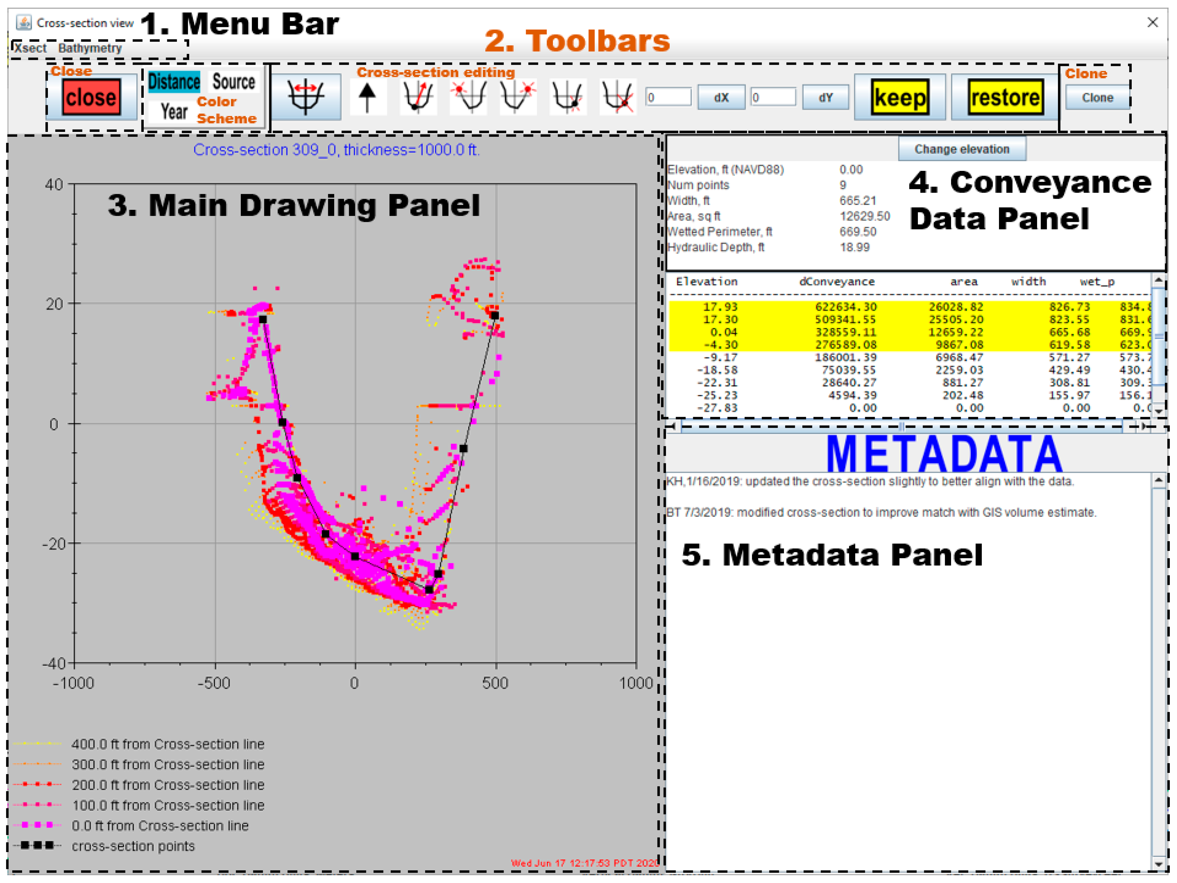
A cross-section window displays bathymetry data in cross-section view, and allows the user to draw a line approximating the shape of the cross-section (
Figure 3). The procedure for opening a cross-section window is as follows: (1) click on a channel centerline to select the centerline (the centerline will then have dots displayed at each centerline point (
Figure 2), (2) click on a cross-section line to select the cross-section line (the cross-section line will then have dots displayed at each of the cross-section line endpoints), and (3) click the "view cross-section” button (
Figure 2, rightmost button in the editing toolbar).
The cross-section window of the CSDP contains five main components: a menu bar, a set of toolbars, a main drawing panel, a conveyance data panel, and a metadata panel. The menu bar contains two menus. The Xsect menu is for saving an image of the window to a file, and for exiting the window. Upon exiting, if there are any unsaved changes to the cross-section drawing, the user will be prompted to save or discard the changes. The bathymetry menu is for changing the size of bathymetry points and changing the color scheme of the bathymetry points.
The cross-section window includes four toolbars, which provide easy access to some of the functions accessible via the menu bar. The close toolbar includes a button for closing the cross-section window. The color scheme toolbar is for selecting a color scheme for the bathymetry data points. The cross-section editing toolbar is for creating and editing the cross-section drawing. The remaining buttons activate the various edit modes. When an edit mode is activated, the button’s background will change from white to yellow, and mouse clicks or drag events on the main drawing panel will perform the corresponding operation. The arrow button on the left hand side of the cross-section editing toolbar turns off edit modes. The remaining buttons from left to right activate the following editing modes: move cross-section point, add left-side cross-section point, add right-side cross-section point, insert cross-section point, and delete cross-section point. The cross-section editing toolbar also includes buttons labeled “dX” and “dY”, each with a text field. Entering a value into one of the text fields and clicking the corresponding button will add the value to each of the “x” or “y” coordinates on the graph. This function can help compare the cross-section drawing to datasets that may not be aligned well with each other, due to data inaccuracies or differences between datasets as a result of changes in the physical system over time. The cross-section editing toolbar also contains “keep” and “restore” buttons. The “keep” button will save the state of the cross-section in memory. The “restore” button will undo all changes since the last time the “keep” button was clicked.
The clone toolbar contains the “clone” button, which will remove all the points in the current cross-section window, replacing them with the points from another cross-section.
The main drawing panel displays selected bathymetry data viewed from the upstream end of the centerline segment to the downstream end, so that data on the left bank appear on the left-hand side of the graph, and data on the right bank appear on the right-hand side of the graph. The cross-section drawing consists of the line segments connected by points in black, which are created by the user by clicking on the graph. Editing (adding, deleting, moving) points can be achieved via checking on the corresponding icons in the toolbar of the cross-section window and then clicking the desirable places in the main drawing panel.
The upper portion of the conveyance data panel displays conveyance characteristics values for a specified elevation. Clicking the “Change elevation” button will allow the user to change this elevation. The lower portion of the panel displays a table of conveyance characteristics for every elevation in the cross-section. Rows in the table that intersect a user-specified range of water levels, intended to represent the intertidal zone, are colored yellow.
The metadata panel in the cross-section window allows the user to enter metadata. Metadata document why a cross-section was drawn the way it was, in order to prevent a future user from making changes without understanding the previous user’s goals in creating the cross-section. Users are encouraged to create or update metadata every time a cross-section is created, reviewed, or edited, including the following information regarding the creation, review, or edit: (1) date, (2) user name or initials, (3) datasets that were prioritized in creating/editing the cross-section drawing, and (4) an explanation of any deviations in the cross-section drawing from the bathymetry data. Metadata are especially important when creating a cross-section that does not align with bathymetry data. There are a number of reasons for creating a cross-section that does not align with bathymetry data, including: (1) to simulate proposed changes in channel geometry, such as dredging, (2) to exclude abrupt changes in geometry that would impact the convergence of the model, and (3) to adjust channel volume to match a GIS volume estimate.
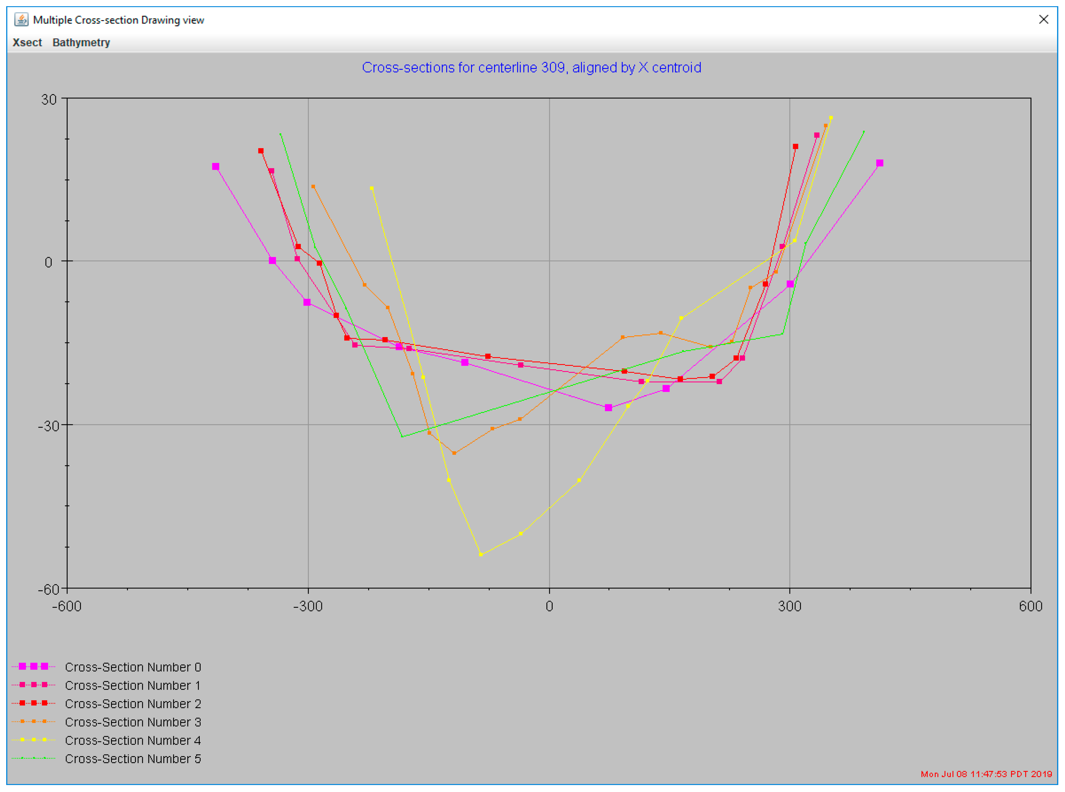
All cross-section drawings in a given channel (centerline) can be viewed together in a multiple cross-section graph (
Figure 4). The graph is created by first selecting a centerline in the CSDP main panel, then selecting the menu item “Centerline–Multiple Cross-Section Graph”. In the graph, all cross-section drawings are centered horizontally by the cross-section X centroids. This multiple cross-section graph can help the user to: (1) understand how shape and cross-sectional area vary along the channel; (2) identify sudden changes in geometry, such as narrow deep holes; and (3) locate errors in cross-section drawings.
3.3.2. Three-Dimensional Cross-Section Plot
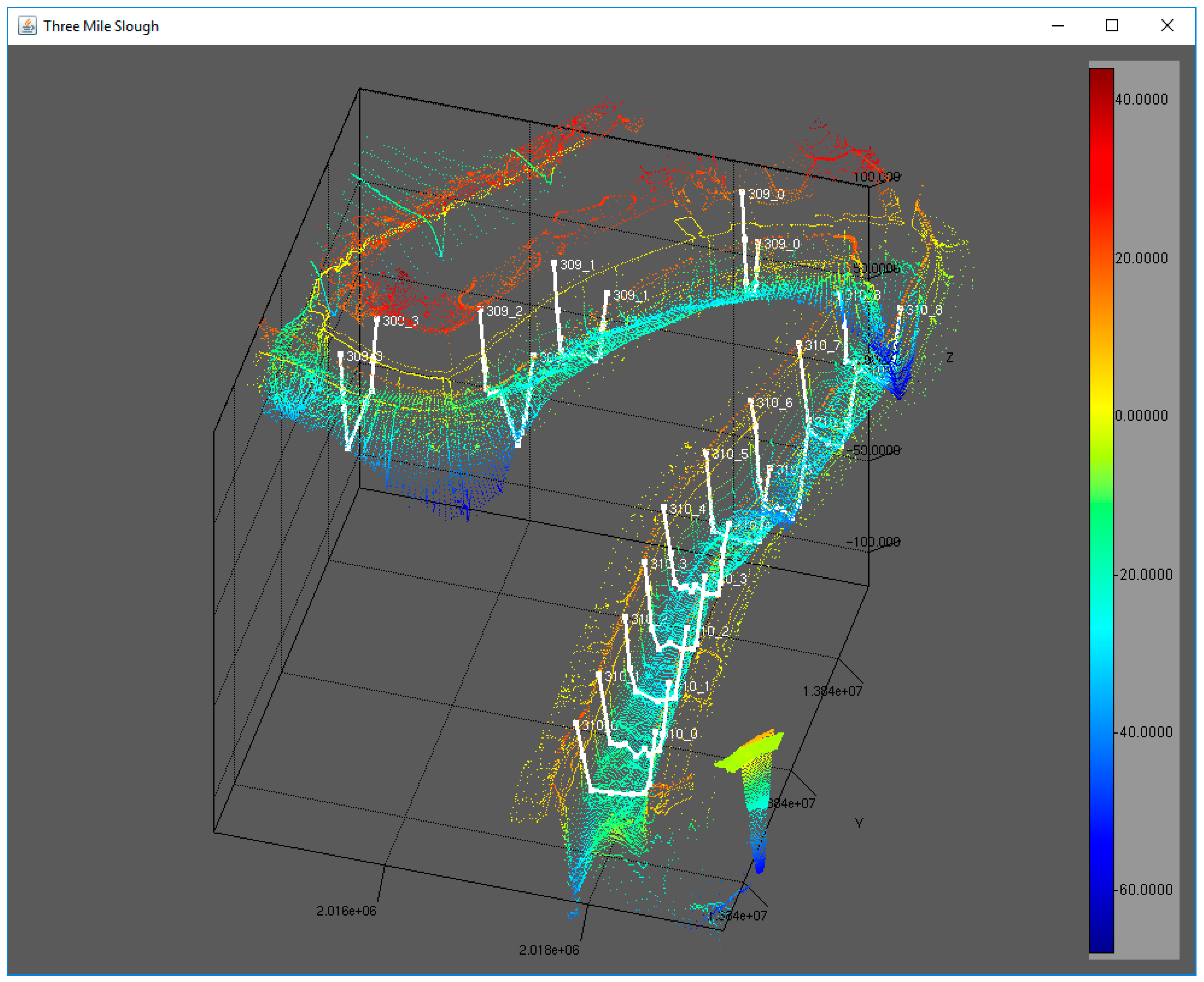
Bathymetry data and cross-sections for a specified channel, reach, or geographical region can also be displayed in three-dimensional (3D) view. The plot can be created by selecting the menu items “Network-3D Plots”, “Centerline-Centerline 3D View” or by clicking one of the buttons in the 3D View toolbar (
Section 3.2).
Figure 5 shows an example 3D plot of bathymetry data (in colorful points) and cross-sections (in white lines). The user can rotate, pan, and zoom the plot in three dimensions to gain a better understanding of the variations in the shape of the channel. This plot can help the user verify that the cross-sections are including/excluding all the physical features (represented by bathymetry data), which should be included/excluded. The user can also determine if cross-sections are likely to accurately approximate the channel volume and identify deep narrow holes that the user may wish to exclude from the cross-sections.
3.3.3. Cross-Section Slideshow
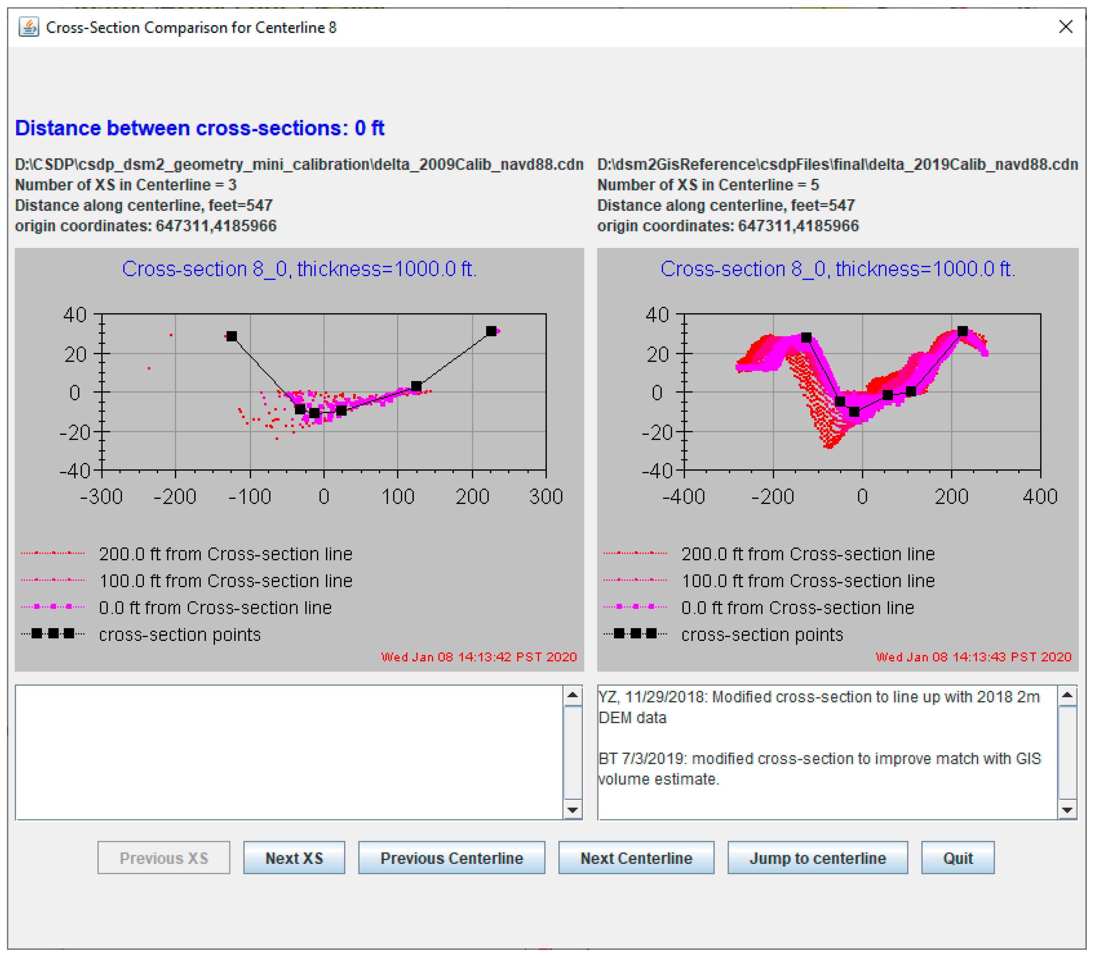
The CSDP cross-section slideshow (
Figure 6) displays windows with two cross-section plots side by side. The two plots display user-created cross-sections from two different network files, and bathymetry from either two different bathymetry files or from the currently loaded bathymetry file. This tool can show how cross-sections differ between two network file versions. Cross-sections are matched by proximity, determined by comparing the locations of the intersections of the centerline segments with the cross-section lines. The window is opened by selecting the “Tools-Cross-Section Slideshow” menu item.
3.4. Geometry Fine-Tuning
Once the geometry (i.e., centerlines and cross-sections) is roughly determined via the aforementioned CSDP functions, it can be imported into the target hydrodynamic models. To make the model run successfully and meaningfully, however, the geometry may need to be fine-tuned for several practical reasons. Firstly, geometry-related convergence issues in hydrodynamic models can arise when a channel has large variations in a cross-sectional area. Secondly, some hydrodynamic models are not designed to simulate channels drying up. The potential causes include: (1) convergence failures can be sufficient to cause oscillations in calculated stage values of increasing amplitude (also known as “blowing up”), (2) an initial stage value that is too high can cause model solvers to overcompensate, calculating a stage value near the beginning of a simulation that is below the bottom of a cross-section, (3) errors in model inputs can result in the model removing all water from a channel, and (4) the model is not designed to simulate conditions that would result in a channel drying up or almost drying up in reality (if a channel comes close to drying up in the model, the model may dry up while iterating to find a solution). Thirdly, the channel volumes determined from CSDP cross-sections need to mimic the actual channel reasonably well. This is typically achieved by matching CDSP channel volumes with channel volumes determined from other techniques. Among all existing software, ArcGIS is probably the most popular one applied widely in calculating channel volumes for hydraulic and hydrodynamic models. The CSDP uses ArcGIS-derived (via Cut Fill calculation) channel volumes as the benchmark and tried to match it as much as possible. The CSDP includes functions to support the user in adjusting geometry to eliminate any potential geometry-related model convergence issues, prevent channels from drying up, and match GIS channel volume estimates. Some of the critical functions include: (1) a network summary report that contains diagnostical metrics that can guide users in geometry fine-tuning; (2) a centerline summary showing the variations of area, width, wetted perimeter, and bottom elevation along a specific CSDP centerline; and (3) the 3D bathymetry and cross-section plot (
Section 3.3.3).
Geometry-related model convergence issues can be avoided if the areas of cross-sections in a specific channel do not vary dramatically. The CSDP calculates a metric (and exports it to the network summary report) to represent the variability in cross-section areas: maximum area ratio. It is defined as the ratio of the largest to the smallest cross-sectional area. Empirically, maintaining this value to below 2.0 has been found to be sufficient to ensure geometry-related numerical stability.
Channel drying up normally occurs when cross-section bottom elevations are above any calculated minimum stage value in a model run. The CSDP adopts a simple strategy to prevent drying up by creating pseudo-cross-section bottom elevations. The following geometry adjustment procedure can help prevent channels from drying up:
Determine a historical minimum stage value for each channel, using historical data or output from a long-term historical hydrodynamics simulation.
Use the CSDP Network Summary Report to compare this value to the lowest CSDP bottom elevation for each channel.
Lower cross-section bottom elevations that are less than about 0.6 m (2 feet) below the historical minimum stage value. For channels that dry up or come close to drying up, these adjustments may involve adding a narrow “V” shape (
Figure 7) to the bottoms of the cross-sections. The “V” shape added in this example is defined by 3 points; the lower point has an elevation of approximately −2 feet, and the upper two points have an elevation of approximately 1.3 feet. There is very little distance between the upper two points, and on the graph, they appear to be plotted almost right on top of each other. The narrow “V” shape lowers the bottom elevation of the cross-section to help prevent drying up, while adding very little cross-sectional area.
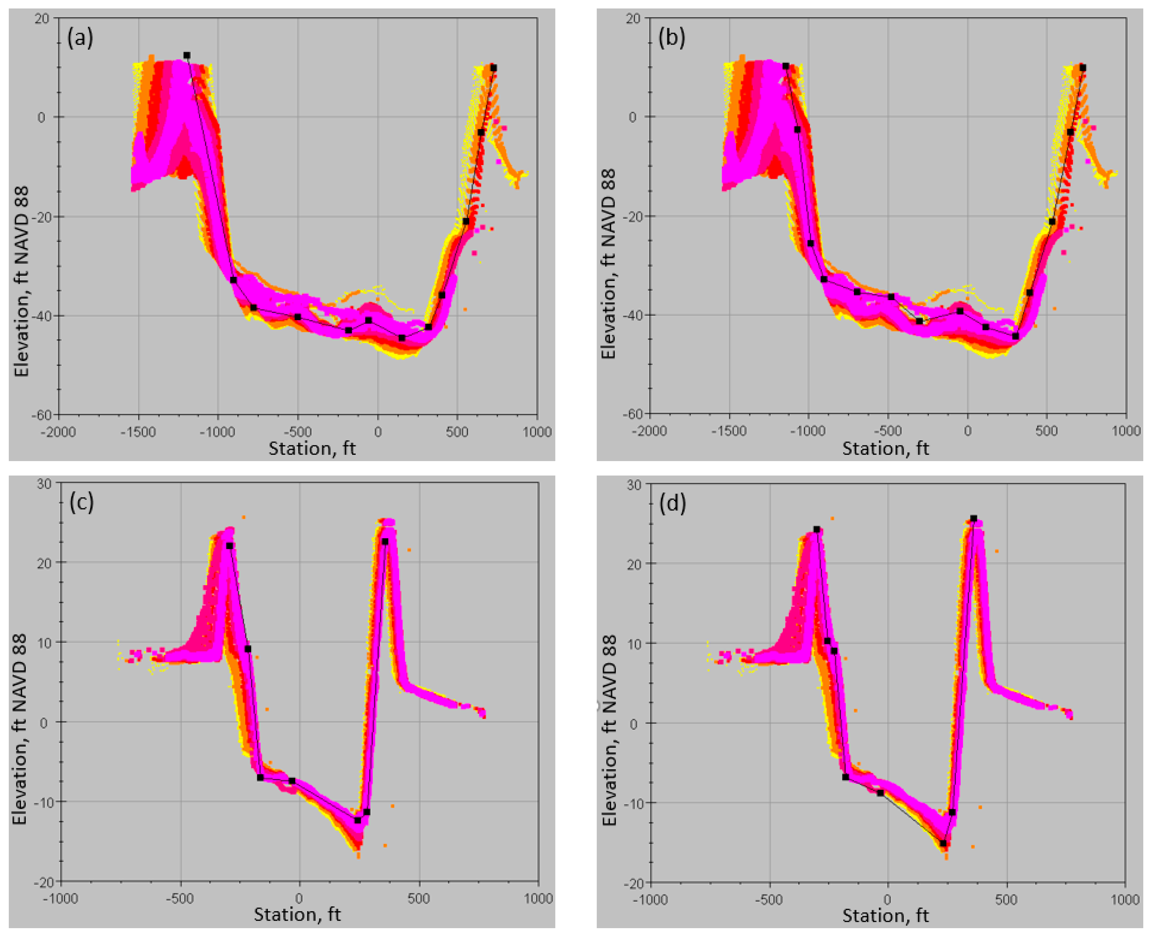
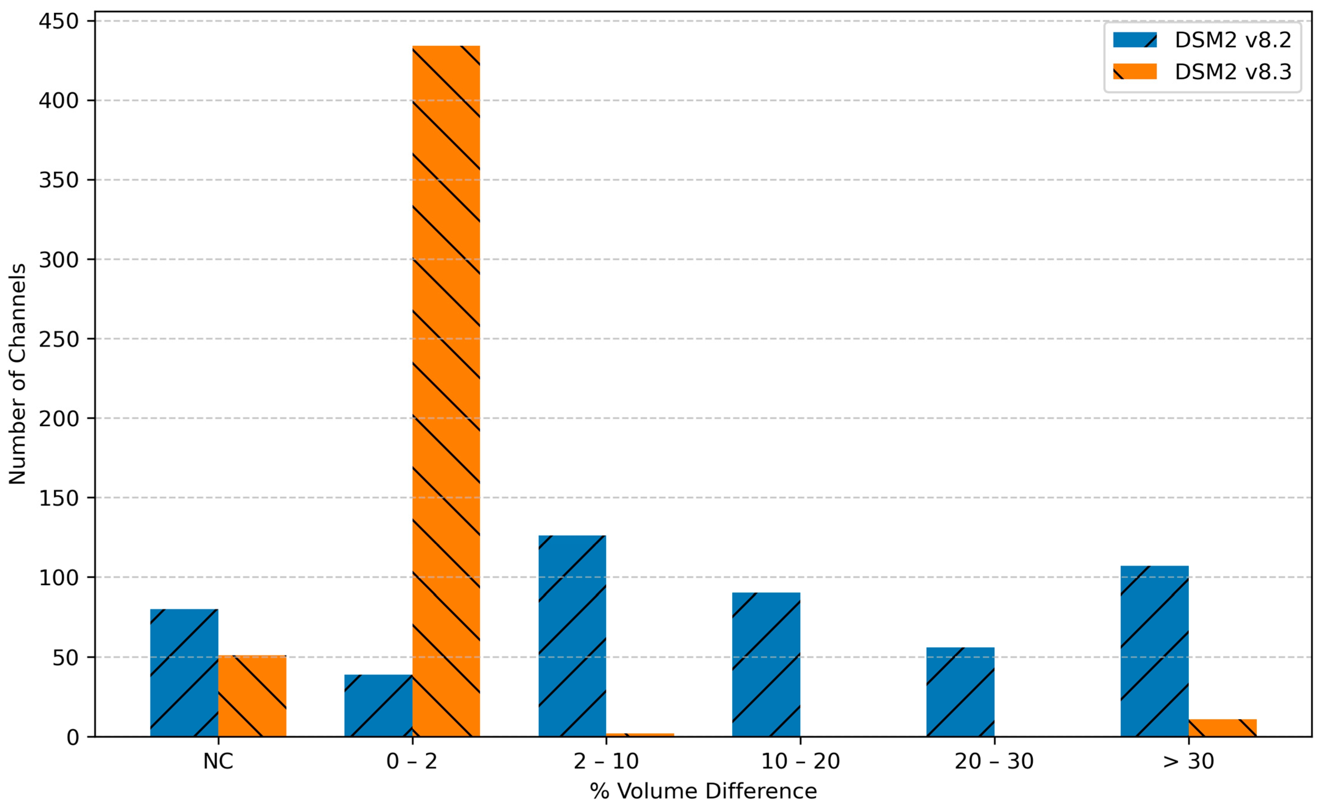
Adjusting cross-sections to match GIS volume is an iterative process, which involves modifying cross-sections, re-creating the Network Summary Report, comparing CSDP and GIS volumes tabulated in the report, and repeating the steps as needed. A cross-section represents not a single location, but a portion of the channel between model computational points. Therefore, to match channel volume, a cross-section drawing should not necessarily align perfectly with the bathymetry data that are closest to their location longitudinally. To keep cross-sections as realistic as possible while matching the channel volume, recommended cross-section adjustments may involve either: (1) moving cross-section points within the cloud of bathymetry points (
Figure 8a,b), or, if necessary, (2) moving cross-section points outside the boundary of the cloud of bathymetry points while maintaining a similar shape (
Figure 8c,d). Increasing the cross-section thickness in straighter channels can enlarge the cloud of points, making it easier to create a representative cross-section.
5. Conclusions and Future Work
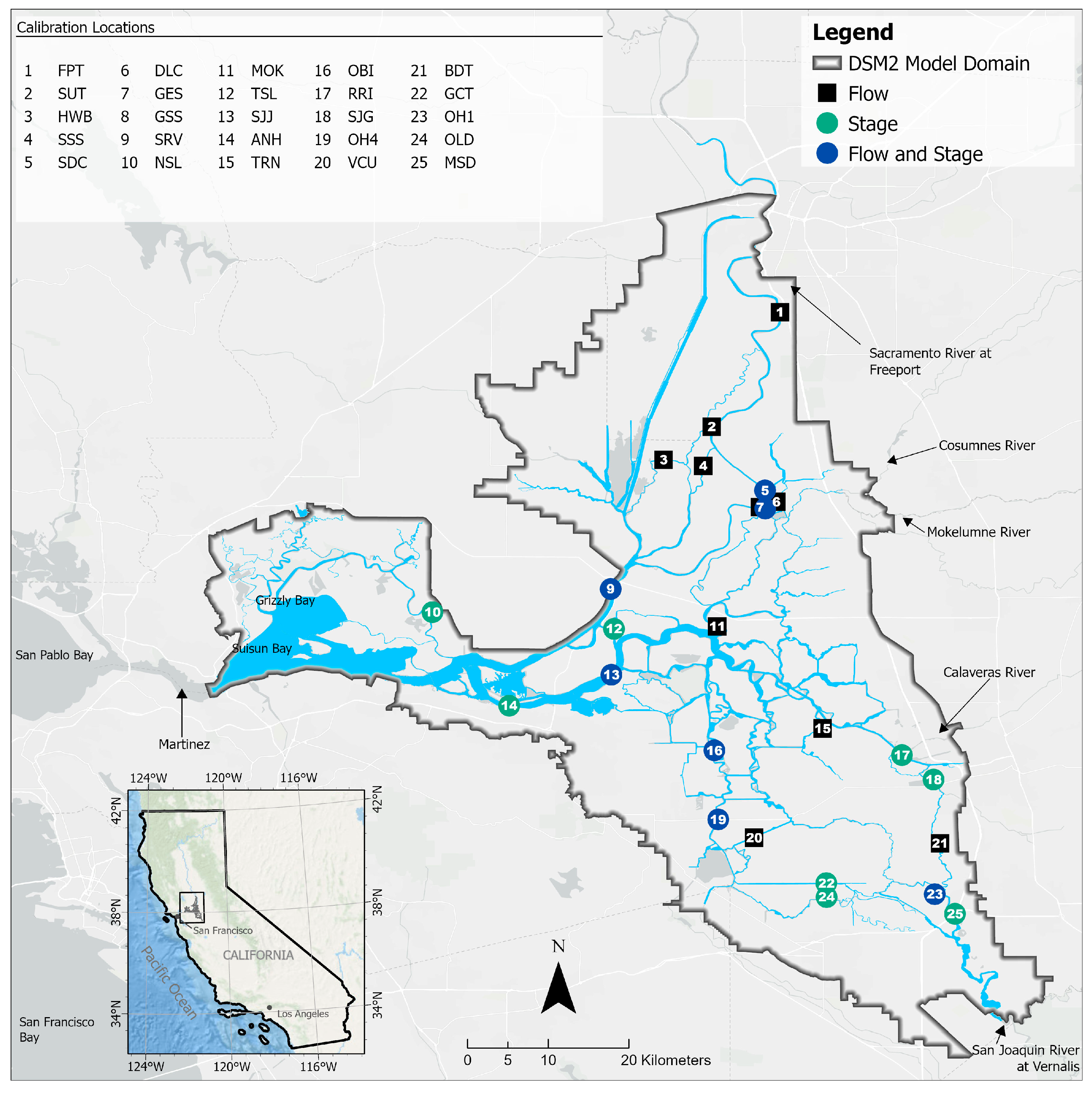
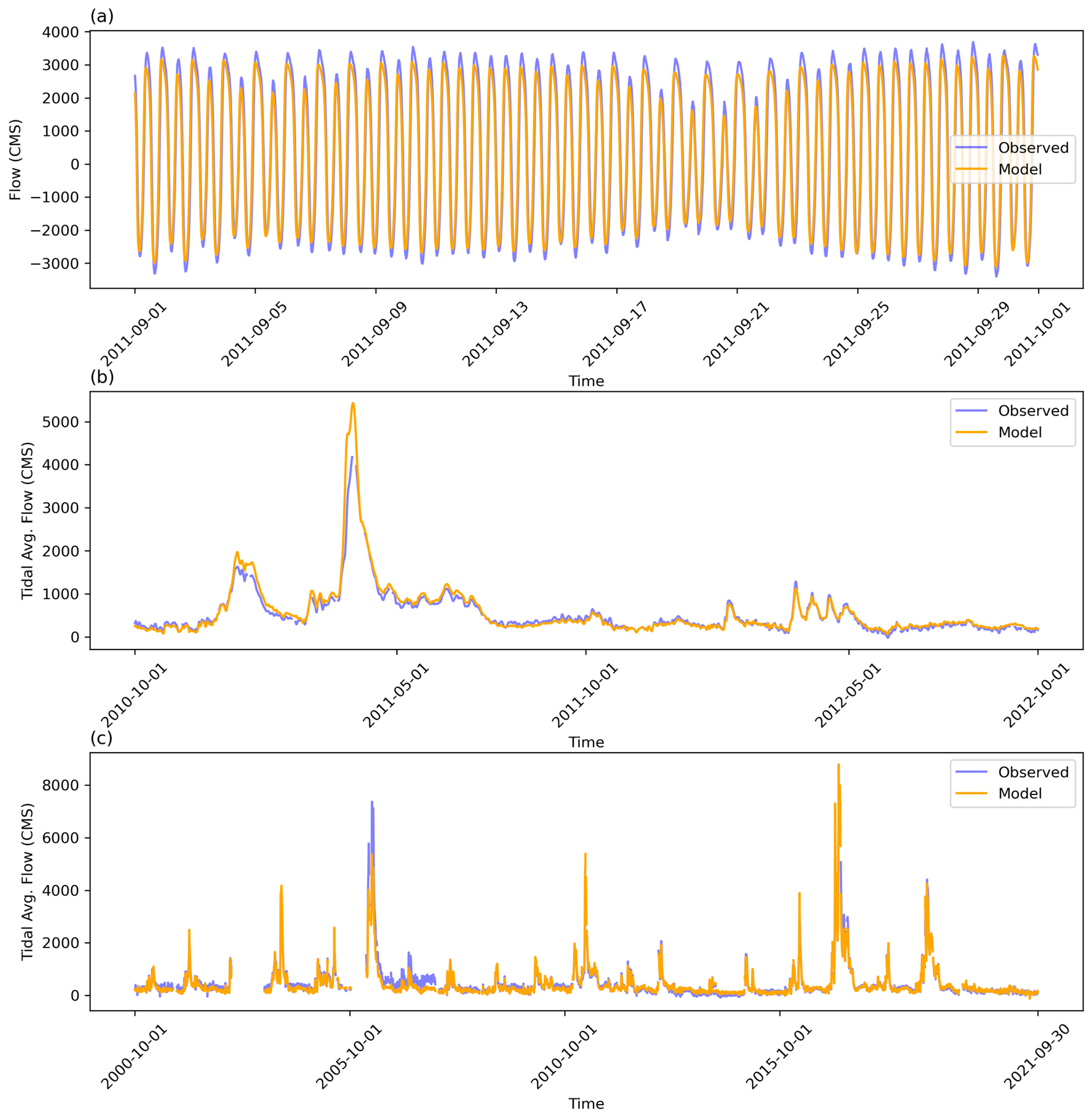
Geometry for some hydrodynamic models consists of cross-sections that are defined at discrete locations in each channel in the model grid. The current study described a parsimonious modular tool, the Cross-Section Development Tool (CSDP), that prepares geometry inputs for hydrodynamic models that use cross-section input. It provides the user with full control over the placement of channel centerlines, cross-section lines, and cross-section points, optionally automating parts of the process. This enables the user, when creating cross-sections, to place more emphasis on datasets considered to be of higher quality, to design cross-sections to evaluate the effects of proposed changes, such as dredging, and to adjust cross-sections as needed to adjust channel volumes. The CSDP also includes tools to help the user identify cross-sections that could potentially cause model convergence issues. The study further demonstrated the application of CSDP in an operational hydrodynamic model (DSM2). We illustrated that the channel volumes derived from CSDP was able to match GIS-based channel volumes and that the model performed well with the updated geometry. Flow and stage simulations from DSM2 configured with updated geometry from CSDP at study locations are compared to the corresponding field observations. Overall, these simulations mimic the patterns of the observations very well. The square of the correlation coefficient between simulations and observations is generally over 0.95 during the calibration period and over 0.80 during the validation period. The absolute bias is generally less than 5% and 10% during the calibration and validation periods, respectively.
By virtue of the modular design, the CSDP could be used to create geometry input for any hydrodynamic model using similar input in any region, provided there are bathymetry data, for example, surveyed DEM or remote sensing data, available for the region of interest. The general procedure would be the same: (a) format the bathymetry data for the CSDP, (b) load the bathymetry data into the CSDP, (c) create cross-sections using the CSDP, and (d) calculate cross-section conveyance characteristics. We plan to continue enhancing CSDP in future releases. Planned enhancements include: (a) more GIS-like GUI; (b) base map display; (c) improving zooming in plan view; and (d) improving interface for centerline and cross-section editing, including undo and redo.
Automated approaches to cross-section development are very efficient, but they require high quality data. Automated approaches are not applicable to the entire California Bay-Delta system, due to the variability in bathymetry data quality. To the best of our knowledge, no other tools have been successful in creating model geometry for the entire California Bay-Delta System. CSDP takes more time than the automatic approach, but it is more efficient than the manual approach to developing cross-sections used by DSM2′s predecessor. The approach used by the CSDP also allows the user, when developing geometry, to use their personal knowledge of the system, improve the numerical stability of hydrodynamic models that use the geometry, and include effects of proposed changes in geometry.
