Review

A Review on the Mixing Quality of Static Mixers

by
Lukas von Damnitz
and
Denis Anders
*
Group for Computational Mechanics and Fluid Dynamics, Cologne University of Applied Sciences (TH Köln), 51643 Gummersbach, Germany
*
Author to whom correspondence should be addressed.
ChemEngineering 2025, 9(6), 128; https://doi.org/10.3390/chemengineering9060128
Submission received: 12 September 2025 / Revised: 7 October 2025 / Accepted: 30 October 2025 / Published: 12 November 2025

Abstract

Static mixers are widely used devices for efficient fluid mixing, homogenization, and enhancement of heat transfer, with applications ranging from chemical processing and pharmaceutical manufacturing to wastewater treatment. This review provides a structured overview of mixing processes and the key metrics used to assess mixing quality in static mixers. Conceptual models such as dispersive versus distributive mixing and the classification into macro-, meso-, and micromixing are introduced as a basis for understanding mixing phenomena. Subsequently, a comprehensive set of quantitative measures, including G-value, residence time distribution, intensity of segregation, coefficient of variation, striation-based descriptors, Lyapunov exponent, extensional efficiency, and shear rate, is discussed in detail. Correlations and relationships among these measures are highlighted to facilitate their application in characterizing mixing quality in static mixers. By systematically summarizing the theoretical background, definitions, and interconnections of mixing quality measures, this review aims to provide researchers and engineers with a clear framework for evaluating and comparing mixing quality in static mixers, thereby supporting both academic studies and practical design considerations.

1. Introduction

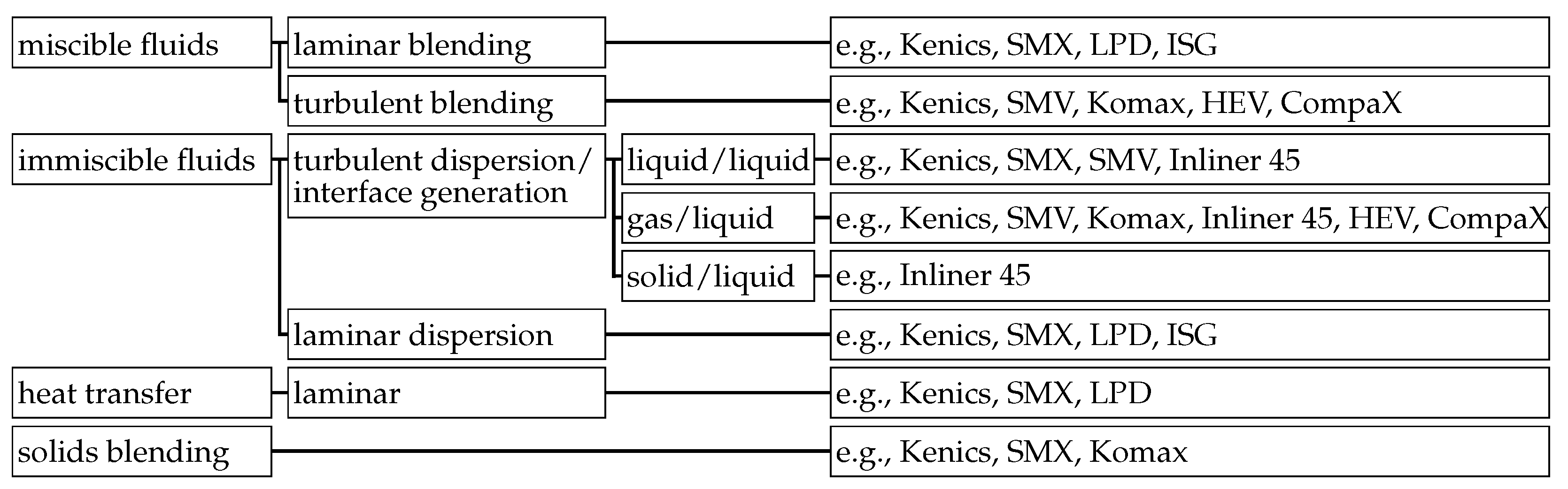
Static mixers are essential components in process engineering that utilize the flow energy of the working fluid to homogenize concentrations and temperatures or to distribute particles, droplets, and bubbles (phase interfaces). They are applied in the mixing of miscible fluids as well as in the dispersion and emulsification of immiscible fluids [1,2]. Further applications include enhancing mass and heat transfer [3,4,5,6,7,8,9] and promoting chemical reactions [10,11,12]. An overview of the various areas of application of static mixers is shown in Figure 1.
Static mixers have been patented since the late 19th century [14,15,16,17], with early developments by petrochemical companies for internal use [13,18,19,20,21]. They gained industrial relevance in the 1970s, particularly after the commercial launch of the Kenics mixer in 1971 [1], and became standard equipment in process engineering [13,21,22]. By the beginning of the new millennium, over 2000 US patents and 8000 scientific publications addressed static mixers, with more than 30 commercial designs available [1,13]. Unlike dynamic mixers, mixing occurs via stationary elements that split, redirect, and recombine the flow, inducing turbulence and radial mixing.
Due to the absence of electrical or moving parts, static mixers are energy efficient, low maintenance, easy to integrate (compact, compatible with existing pipes) and cost-effective [13,21,22,23]. Unlike batch-operated dynamic mixers, they enable continuous processing [23]. Static mixers can be designed for cleaning in place or rapid replacement, simplifying maintenance [13]. They require only short residence times and pipe lengths, promote plug flow, and allow fast product changeovers with minimal waste [13,21,22,23]. In contrast to dynamic mixers, which can damage products due to localized high shear, static mixers achieve effective mixing even at low shear rates [13].
Due to their versatility (miscible/immiscible fluids, gas/liquid phases, high/low viscosities, laminar/turbulent flow) and process advantages, static mixers are widely used in chemical, pharmaceutical and food industries, as well as in power plants and water treatment [1,21]. Please note that the present review does not address specific regulatory or performance thresholds, which can vary considerably between applications. Instead, the focus is placed on the definitions of mixing quality measures and the correlations of these measures across different static mixer types.
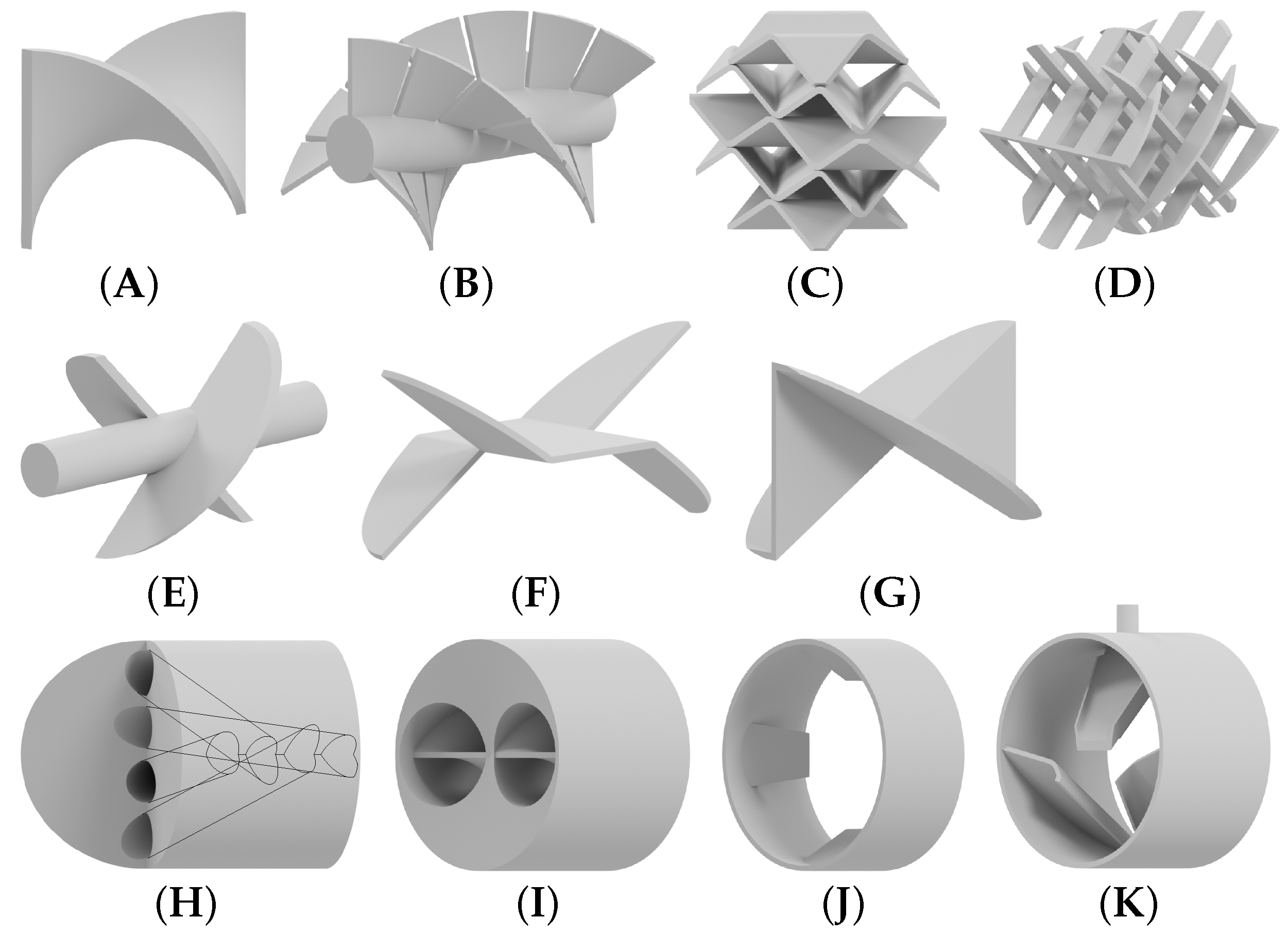
However, the design of static mixers strongly depends on the specific application scenario, leading to a wide variety of mixer types. Designs featuring alternating helical elements, such as Kenics, Inliner 50 or Hi-mixer, are among the most widely used [1]. For inducing strong turbulence and vortex formation, types with angled blades or baffles mounted to the pipe wall have been developed [1], e.g., High Efficiency Vortex mixer (HEV), Low Pressure Drop mixer (LPD), Komax, CompaX, Inliner 45 (also called Cleveland).
Static mixer types designed primarily for turbulent flows employ layered corrugated plates to generate local acceleration and elongation of the fluid, e.g., SMV [1]. Types with multilayered grids or tube structures divide the flow into many substreams, enabling distributive mixing by convection, e.g., SMX and KMX (which has the same layering as the SMX, but with curved blades) [1]. Channel-based designs typically split, twist, and laterally shift fluids in separate paths before recombining them in offset layers, e.g., Interfacial Surface Generator (ISG), Hi-mixer [1]. Another design variant, based on a grid of varying geometries that superimposes a highly turbulent field onto a quasi-plug flow, is less common in industry but studied in academic research [1,24,25,26,27]. For micromixing applications, such as miniaturization laboratory equipment into a lab-on-a-chip, special small scale static mixers called passive micromixers are developed [28,29]. Figure 2 illustrates the most commonly used and researched static mixers. In general, the mixing elements of static mixers are mirrored and rotated by 90° along the central axis of the pipe to induce chaotic flow, with the exception of ISG, HEV, and CompaX static mixers.
Key criteria for the design and evaluation of static mixers include mixing quality and pressure drop. The mixing quality depends on fluid properties (density, viscosity, diffusivity, etc.), process conditions (flow rate, concentration ratio, shear rate, etc.) and the geometry of the pipe as well as the mixer geometry (diameter, length, etc.).
Early comparisons of static mixers focused on pressure drop [30], and some mixing quality metrics, such as the G-value, were derived from it. It was assumed that higher pressure losses, and thus greater energy dissipation, lead to increased turbulence and shear automatically enhancing mixing quality. In most mixer types, improved mixing quality indeed correlates with higher pressure drop. However, the reverse conclusion is not generally valid, meaning that pressure drop as a single process variable does not reliably indicate mixing quality. One of the first quantitative definitions of mixing quality was proposed by Danckwerts in the 1950s [31]. Since then, numerous other definitions have emerged [23], based on concentration fields, particle or droplet sizes, residence time, flow chaos, and deformation mechanisms. According to these definitions, the different mixing quality measures can be categorized as follows:
The wide range of non-equivalent definitions, varied measurement techniques, and sample-size dependence complicate the interpretation and comparison of mixing quality data in the literature [13,23,33]. Therefore, this contribution aims to provide an overview of the most commonly used mixing quality measures for static mixers and, where possible, to identify relationships among them. The review focuses on the mixing of miscible fluids, with the objective of providing a fundamental understanding of the mixing processes and mixing quality measures, thus offering a structured introduction to the topic. The mixing of multiphase flows using static mixers has been extensively reviewed by other authors [1,13]; however, these reviews have not addressed the mixing quality measures for miscible fluids in the depth intended here. To this end, we first discuss conceptual models and classifications of the mixing process. Subsequently, key mixing quality measures are introduced, along with relevant correlations and methods for evaluating the most widely used industrial mixer types.

2. Mixing Processes and Metrics for Mixing Quality

2.1. Conceptual Models and Classifications of Mixing

Mixing in static mixers involves various interacting mechanisms. For this reason, several authors have proposed dividing the overall mixing process into distinct subprocesses [2,13,21,30,31,40,43,55,56,60,70,71,72,73,74,75,76]. In the next sections, different views on mixing as well as the basic mixing mechanisms are presented.

2.1.1. Dispersive vs. Distributive Mixing

Danckwerts distinguished two fundamentally different and independent mechanisms in the (laminar) mixing of fluids, each contributing differently to the overall mixing outcome [31]:
  • The division and stretching of fluid regions with uniform composition,
  • Diffusion across the interfaces between regions of differing composition.
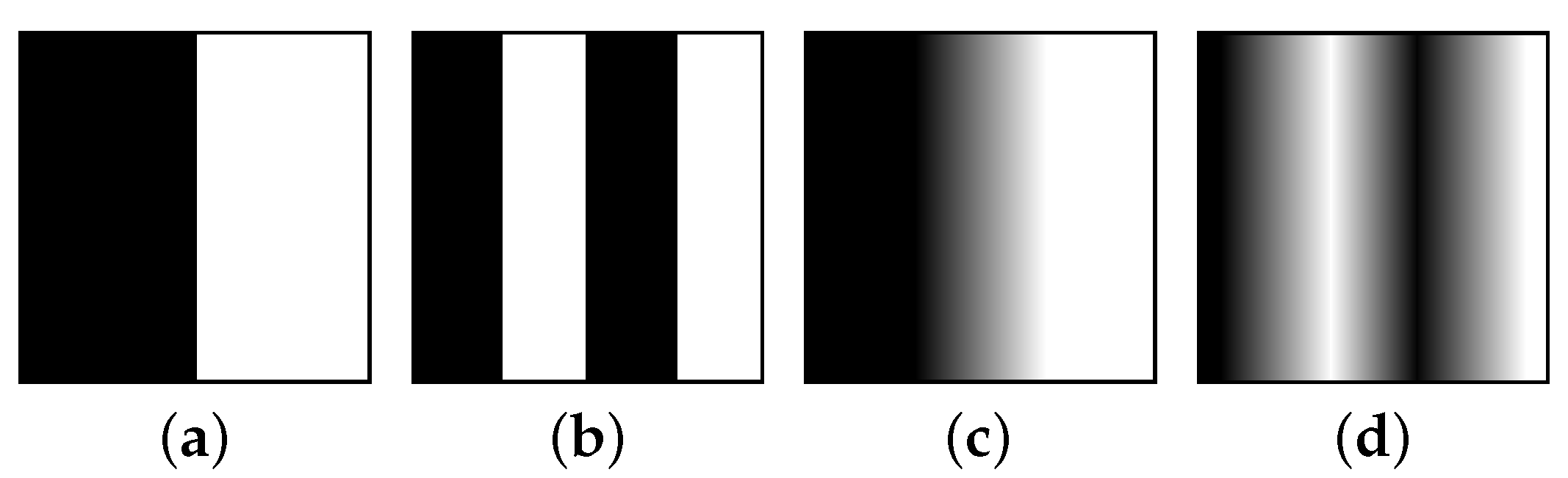
Stretching and dividing fluid regions alone cannot produce a homogeneous mixture, as concentration differences between regions remain without diffusion (or equivalent processes such as heat conduction or turbulence). As illustrated in Figure 3b, these regions remain separated by distinct concentration interfaces [31].
A homogeneous mixture can only be achieved through diffusion (or equivalent mechanisms), as shown in Figure 3c. However, diffusion is inherently slow. Since the rate of diffusion depends on the interfacial area between regions of differing concentration, increasing this area, through division and stretching, reduces the time required for homogenization; see Figure 3d.
To characterize these two effects, Danckwerts introduced two distinct metrics for mixing quality: the scale of segregation and the intensity of segregation [31]. A similar classification of laminar mixing processes, neglecting turbulence and diffusion, was proposed by Spencer & Wiley [43]. They described mixing as a result of continuous deformation, composed of two subprocesses:
  • Increase in the interfacial area between the fluids (or division of the material),
  • Distribution of these interfaces within the volume (or redistribution of the subdivided material).
The process of generating progressively smaller domains is referred to as dispersive mixing, whereas achieving a more uniform spatial distribution is termed distributive mixing [2,30,55,60]. These concepts are also employed in the context of turbulent mixing [40]. In contrast, some authors define distributive mixing as the mixing of miscible fluids and dispersive mixing as the mixing of immiscible fluids [13,21].
Based on the classifications by Danckwerts [31] and Spencer & Wiley [43], metrics for mixing quality can be grouped into two categories: those that quantify the size of unmixed regions or interfaces (e.g., scale of segregation, striation thickness, interfacial area) and those that evaluate concentration variations (e.g., intensity of segregation, coefficient of variation and other variance-based metrics). Since chemical reactions, diffusion, and heat conduction depend on the concentration differences across interfaces as well as the interfacial area itself, Kukukova et al. [34] introduced a third metric: exposure. This measure captures the rate or potential of segregation reduction (i.e., the rate of change of segregation) and is particularly relevant for reactive or complex mixing processes. Exposure thus bridges the concepts of dispersive and distributive mixing by accounting for both interface characteristics and concentration gradients.

2.1.2. Macro-, Meso- and Micromixing

Macro-, meso-, micromixing is an alternative conceptual framework to describe mixing mechanisms by Villermaux & David [56], Baldyga & Bourne [72,73,74] and Fournier et al. [75,76]. Villermaux & David divided the mixing process in reactors into macromixing and micromixing stages and proposed a quantification based on the characteristic time scales and the micromixedness ratio, defined as the ratio of micromixed to macromixed portions within the mixture [56]. Notably, macro-, meso-, and micromixing can occur concurrently and interactively during the mixing process [56,71].
(a)
Macromixing
Macromixing refers to the initial stage in which components are distributed throughout the entire reactor or static mixer volume, also referred to as the volume filling stage [71]. During this phase, the average concentration is homogenized on the scale of the vessel, while local concentration gradients may persist [21,56,70].
This process can be effectively analyzed using computational fluid dynamics (CFD), particularly when high spatial and temporal resolution is available [70]. In continuous reactors, macromixing is often characterized using the residence time distribution (RTD) [21,56]. The sharpness of the RTD, and thus the efficiency of macromixing, can be enhanced through improved radial (convective) transport, such as by introducing longitudinal vortices via vortex generators or baffles that disrupt axial flow [21].
(b)
Mesomixing
Mesomixing describes the intermediate scale reduction stage in which regions of uniform concentration become progressively smaller [71]. It bridges the spatial and temporal gap between macromixing and micromixing [70,71]. However, many authors do not explicitly use the term mesomixing and instead include its effects under the micromixing category [70]. The mechanisms of scale reduction differ between laminar and turbulent flows. In laminar regimes, stretching and folding of fluid elements lead to the formation of a lamellar structure, characterized by an average striation thickness [21,56]. In contrast, turbulent flows produce scale reductions via turbulent erosion [56], also distinguished in turbulent dispersion and turbulent disintegration [74], in which fluid fragments are continuously separated from larger domains and dispersed into the surrounding fluid [56,74].
(c)
Micromixing
Micromixing refers to the final stage of the mixing process, dominated by molecular viscosity and diffusion (diffusion stage), and occurs at the smallest spatial and temporal scales of motion and concentration [21,56,70,71].
Various characteristic length scales are proposed in the literature to define the regime in which molecular diffusion becomes dominant. Among the most common are the Kolmogorov scale l K , which denotes the smallest eddy size at which turbulent kinetic energy is dissipated [21,56,71], and the Batchelor scale l B , which characterizes the scale at which scalar (e.g., concentration) gradients are smoothed out by diffusion over the lifetime of a Kolmogorov-scale eddy [56,70].
The Kolmogorov scale l K typically is between 5 and 50 µm in industrial processes [13,21] and is calculated using Equation (1) [56]:
l K = ν 3 ϵ 1 / 4
where ν is the kinematic viscosity ( ν = μ / ρ ), and ϵ is the average turbulent energy dissipation rate per unit mass. The Batchelor scale l B is defined by Equation (2) [56]:
l B = ν D diff 2 ϵ 1 / 4 = l K Sc
where D diff is the molecular diffusivity, Sc is the Schmidt number ( Sc = ν / D diff ), and l K is the Kolmogorov scale.
Due to the extremely small length scales, it is difficult to describe micromixing computationally, even using Direct Numerical Simulation (DNS). Therefore, in simulations of reactive systems, micromixing must often be modeled through sub-grid-scale approaches (micromixing models) that couple macroscopic hydrodynamics with molecular kinetics [70]. It should be emphasized that macromixing, mesomixing, and micromixing are not isolated processes but rather interconnected stages of the overall mixing phenomenon. Large-scale flow structures established during macromixing determine the convective transport patterns that, in turn, generate smaller striations and local fluctuations at the mesoscopic level. These mesoscopic structures form the basis for micromixing, where molecular diffusion finally homogenizes concentration differences within the smallest scales. In static mixers, the strength and efficiency of these coupling mechanisms depend strongly on the geometry and flow regime. Consequently, the quantitative measures discussed in this review are typically associated with specific scales, yet their physical meaning and applicability are inherently linked through these hierarchical interactions.

2.2. Definitions of Mixing Quality Measures

Turbulent mixing is often characterized using statistical quantities such as the local mean and standard deviation of velocity and concentration [71]. In turbulent systems, the phase of initial distribution of the mixing components throughout the entire volume (volume filling or macromixing) proceeds rapidly, while the subsequent phase of reducing the size of regions with uniform concentration (scale reduction or mesomixing) occurs more slowly [71].
In contrast, laminar mixing is limited by diffusion. Here, the macromixing and mesomixing phases do not occur sequentially but rather simultaneously. Effective mixing in laminar flow requires an increase in the interfacial area between regions of different concentration and a decrease in the thickness of individual fluid layers (striation thickness). Consequently, suitable mixing quality metrics must be capable of capturing these fine-scale structures. Statistical descriptors are also used for analyzing laminar mixing; however, the development of practical and robust methods remains an active field of research (as of 2008) [71].
The most useful metric for a given mixing process is the one that shows the greatest variation during the later stages of mixing. For laminar mixing, this typically includes measures that describe the size and structure of segregated regions, such as the scale of segregation or the striation thickness. In turbulent mixing, metrics that describe the strength of gradients between these regions, such as the intensity of segregation or the coefficient of variation (CoV), are more informative [71].

2.2.1. G-Value

The G-value was developed in 1943 by Camp and Stein to quantify mixing in turbulent flocculation basins, based on an analogy to shear rates in a simple, one-dimensional laminar shear flow (Couette flow). It can be easily calculated from numerical models using Equation (3) and has therefore been used to describe macromixing in various mixing applications [68,77].
G = P μ V = V ˙ Δ p μ V = 1 2 π D Re Δ p V ρ
The original derivation of the G-value for three-dimensional flows contains errors. Additionally, G-values are not directly comparable across different mixer types or mixer sizes, identical G-values may yield different mixing outcomes depending on the mixer geometry and scale [77]. The result of mixing quality as represented by the G-value is particularly sensitive to pressure drop. Since volumetric flow rate, fluid density, and dynamic viscosity are typically constant across mixer comparisons, and since mixer volume alone does not indicate mixing quality, the pressure drop dominates the G-value. However, components with high pressure drop, such as orifice plates, can exhibit significantly poorer mixing quality compared to static mixers of the same pressure drop specifically designed for mixing purposes. This indicates that a high pressure drop does not necessarily imply high mixing quality. The G-value is intended to describe the intensity of mixing by relating pressure drop to mean residence time t ¯ = V / V ˙ [78]. For these reasons, the G-value is considered to have limited explanatory power, although it is still used in some cases [68,77,78].

2.2.2. Residence Time Distribution

The residence time t is defined as the time a fluid element or tracer requires to travel a certain distance (e.g., the length of a mixer) [23]. The residence time distribution E ( t ) , introduced by Danckwerts [51], represents the distribution function of all residence times, often normalized by the mean residence time t ¯ . It indicates the fraction of fluid elements or tracers that have traversed the defined path after a residence time t [51].
The cumulative residence time distribution F ( t ) is obtained by integrating the residence time distribution E ( t ) from t = 0 to a specific time t, i.e., it represents the accumulated fraction of fluid elements or tracers that have completed the defined path by time t; see Equations (4) and (5). Consequently, F ( t ) equals 0 at t = 0 and asymptotically approaches 1 as t [51].
F ( t ) = 0 t E ( t ) d t
E ( t ) = d F ( t ) d t
The (cumulative) residence time distribution is a commonly used measure that provides insights into the flow behavior within a static mixer [2], particularly regarding the temporal homogeneity of the mixing process [13,21]. It is especially relevant for chemical reactions and for static mixers that serve as chemical reactors [2,13,58]. Moreover, the residence time distribution is frequently employed to characterize macromixing [21,52,56].
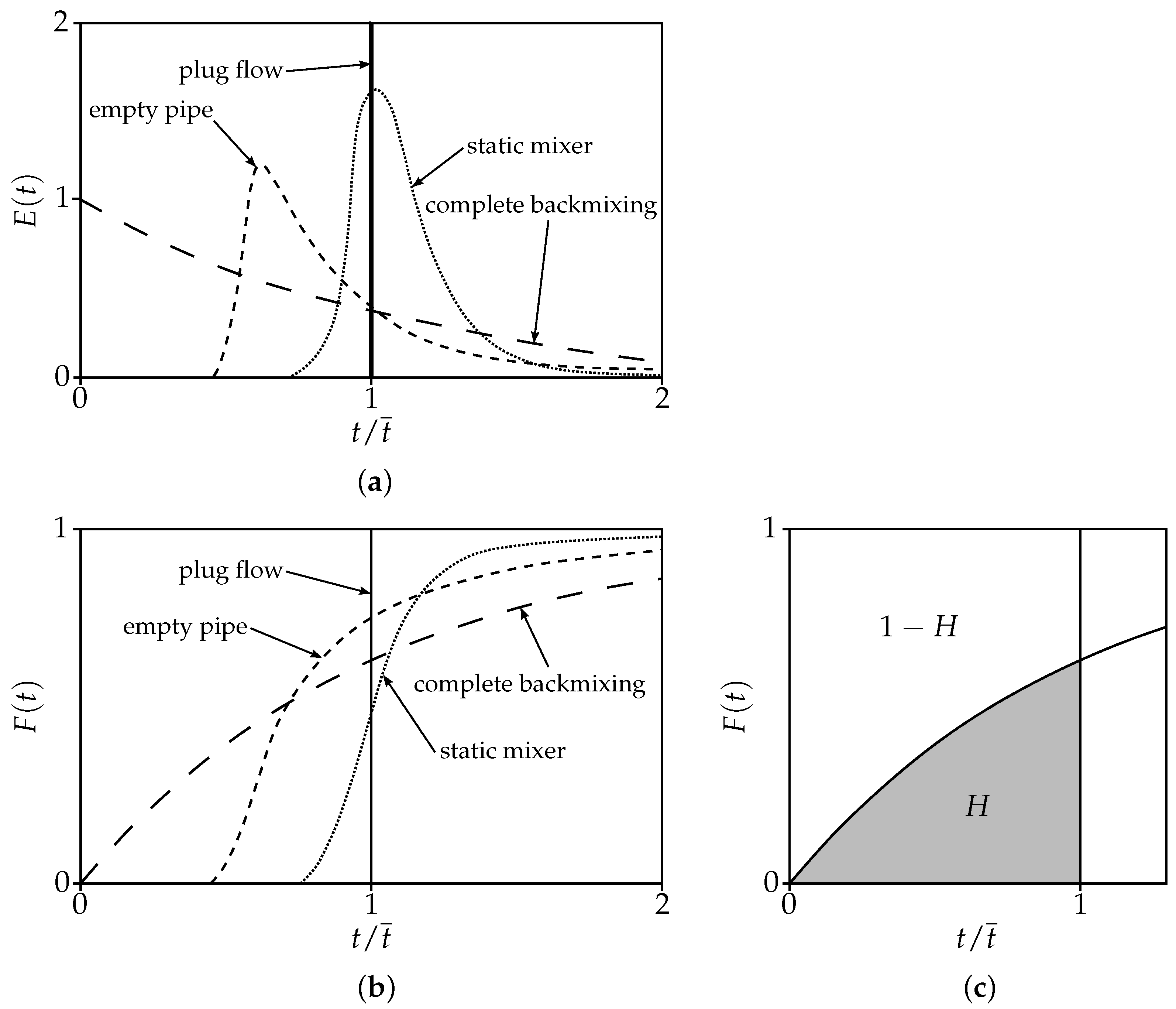
Figure 4 shows the residence time distributions E ( t ) and cumulative residence time distributions F ( t ) for plug flow, complete backmixing, as well as flow through an empty pipe and a static mixer.
The residence time distribution allows for determining whether the flow follows a nearly direct path from the inlet to the outlet, or whether significant portions of the fluid are separated from the main flow, causing fluid elements that entered the mixer at the same time to exit at different times [2].
Ideally, molecules that enter the mixer simultaneously should also exit at the same time, homogeneously mixed. This ideal case is referred to as plug flow and results in a step-shaped residence time distribution at a dimensionless residence time t / t ¯ of 1 [13].
In contrast, under laminar flow conditions, the parabolic velocity profile causes molecules that enter simultaneously to exit at different times, leading to a broad residence time distribution [13].
In general, a narrower residence time distribution indicates better mixing [2]. The broad distribution seen in complete backmixing is detrimental to reactor performance [79,80,81].
Static mixers tend to narrow the residence time distribution [23], bringing it closer to that of ideal plug flow [12,13,23,55].
The degree to which the residence time distribution approaches plug flow can be described using the first appearance time t first , which is the time at which the first tracer (molecule of the mixing fluid) reaches the outlet [13]. This is often expressed as the dimensionless first appearance time t first / t ¯ . The value of t first / t ¯ is 0.5 for laminar pipe flow and 1 for ideal plug flow [13]. If the first appearance time is difficult to measure, the 5% response time, defined by F ( t ) = 0.05 , can be used as an alternative [13]. Another metric for quantifying the deviation from plug flow is the dimensionless variance of the residence time distribution σ t 2 / t ¯ 2 [13,59], shown in Equation (6). It equals 0 for ideal plug flow and theoretically approaches infinity for laminar flow without diffusion [13]. Since diffusion always occurs in real systems, σ t 2 for real laminar flow assumes a finite value [13].
σ t 2 t ¯ 2 = 2 0 [ 1 F ( t ) ] t d t t ¯ 2 1 = 0 t 2 E ( t ) d t t ¯ 2 1
As an alternative to the dimensionless variance, the coefficient of variation of residence time distribution CoV t is also used, which is described by Equation (7) and is likewise equal to 0 for ideal plug flow [59]. In general, the smaller σ t 2 or CoV t , the narrower the residence time distribution and the better the mixing quality [59].
CoV t = σ t t ¯
For the integration of Equation (6), an exponential extrapolation of the measured data is recommended [13]. Danckwerts defined the hold-back H, which quantifies the deviation of the residence time t from the mean residence time t ¯ according to Equation (8) [51].
H = V ˙ V 0 V V ˙ F ( t ) d t = 1 t ¯ 0 t ¯ F ( t ) d t
The hold-back H corresponds to the area under the cumulative residence time distribution F ( t ) between t / t ¯ = 0 and t / t ¯ = 1 (see Figure 4c). For plug flow, H = 0 , and for complete backmixing, H = 1 / e [51].
The residence time distribution is a measure of the temporal homogeneity of mixing [13,21], but it does not reflect spatial homogeneity. Therefore, it is not sufficient on its own as a measure of mixing quality [47,53,54]. To describe spatial homogeneity and the mixing microstructure, other measures must be considered, such as striation thickness, interfacial area, or stretching [13,21,54]. The residence time distribution can be experimentally determined by injecting a tracer pulse at the inlet and measuring the tracer concentration at a cross-section after a defined distance [59].

2.2.3. Distributive Mixing—Describing Gradients Between Segregated Regions

Distributive mixing improves the spatial distribution of particles, droplets, or bubbles [2,30,40,55]. Key evaluation metrics include:
  • Standard deviation of concentration/mixing index [30]
  • Intensity of segregation [60]
  • Coefficient of variance (CoV) [2,39,40,55]
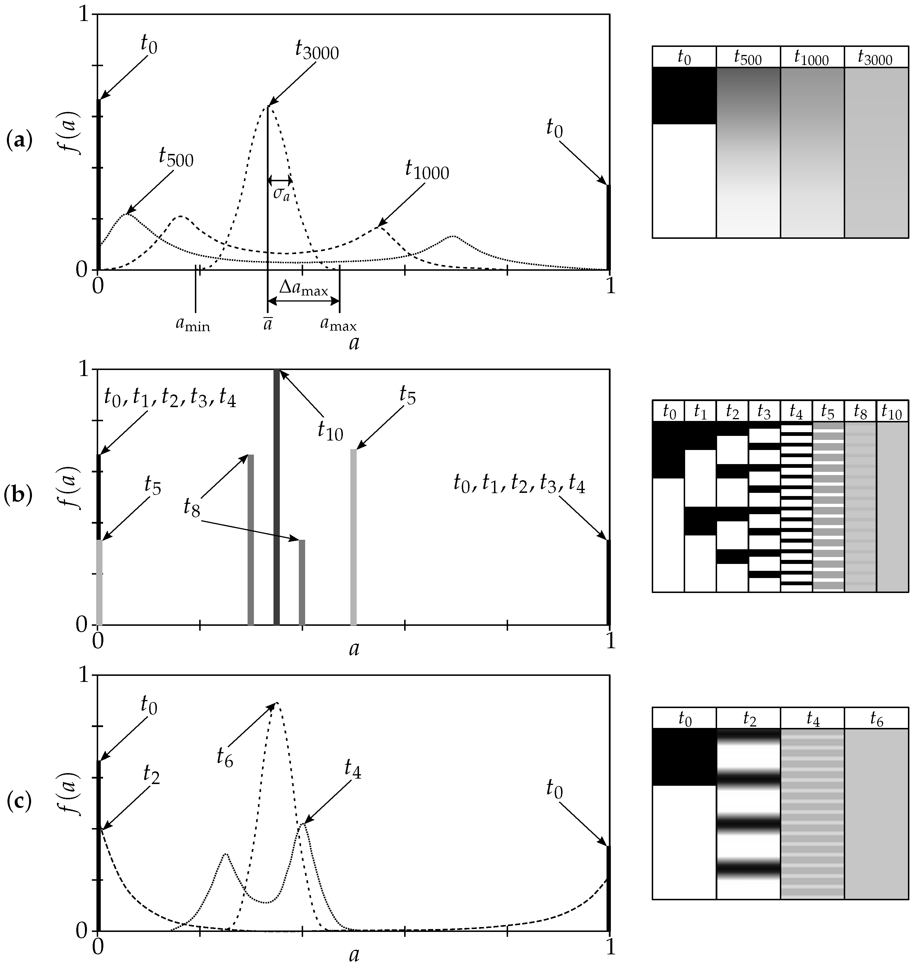
These metrics rely on statistical analysis of the resulting mixture, based on variance, standard deviation, probability density function, or frequency distribution (see Figure 5). For binary mixtures (fluid A with concentration a, and fluid B with concentration b), metrics are symmetrical. Calculations typically use component A, ideally the minor phase ( a ¯ 0.5 ), as a ¯ appears in denominators of several mixing indices [82]. Figure 5 shows the evolution of the frequency distribution f ( a ) during mixing of a 1:2 ratio of fluids A and B based on diffusion (a), mixing through baker’s transformation (b) and a combination of mixing and diffusion (c). Initially ( t 0 ), two distinct peaks at a = 1 (height 1/3) and a = 0 (height 2/3) are visible. As diffusion or mixing with diffusion progresses, the peaks broaden and move toward the mean concentration a ¯ , eventually merging into a single normal distribution (see Figure 5a,c). Further homogenization leads to a single narrow peak at a ¯ with decreasing standard deviation σ a 0 , until full mixing is achieved. During mixing without diffusion, the concentration differences initially do not change, as mixing only separates and spatially distributes the regions of equal concentration. When these regions become smaller than the sample size, they are averaged, forming discrete peaks that converge to a ¯ (see Figure 5b).
In real processes, a fully homogeneous mixture is never achieved, since small concentration variations and distinct domains remain [33]. Mechanical rearrangement (e.g., baker’s transformation) combined with diffusion can significantly accelerate homogenization (see Figure 5c). In this context, Danckwerts’ scale of scrutiny refers to the smallest sample size below which segregated regions are considered mixed [83]. It depends on the application and required level of mixing, but is often limited by the measurement technique [71].
Danckwerts [83] distinguishes between:
  • Coarse grained mixtures: The sample size includes only a few particles or molecules. Even in a perfectly random (fully mixed) system, local concentration differences appear. If a sample contains only one molecule, it can only yield values of 0 or 1 (variance = 1), falsely indicating complete segregation. Nonetheless, this is considered fully mixed since further mixing cannot improve it [83].
  • Fine grained mixtures: The sample size includes many particles, so a perfectly mixed system yields uniform composition across all samples (variance ≈ 0). Incomplete mixing typically requires two parameters for characterization: the scale of segregation (domain size) and the intensity of segregation (concentration difference between domains) [83]. A single measure is often insufficient for describing the mixture [84].
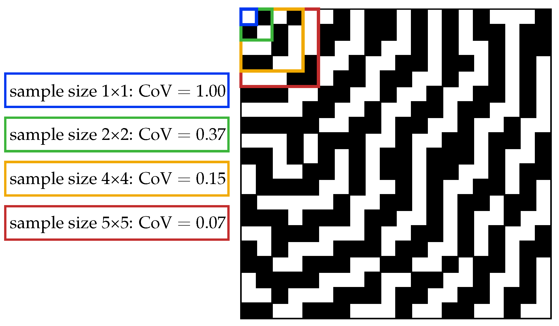
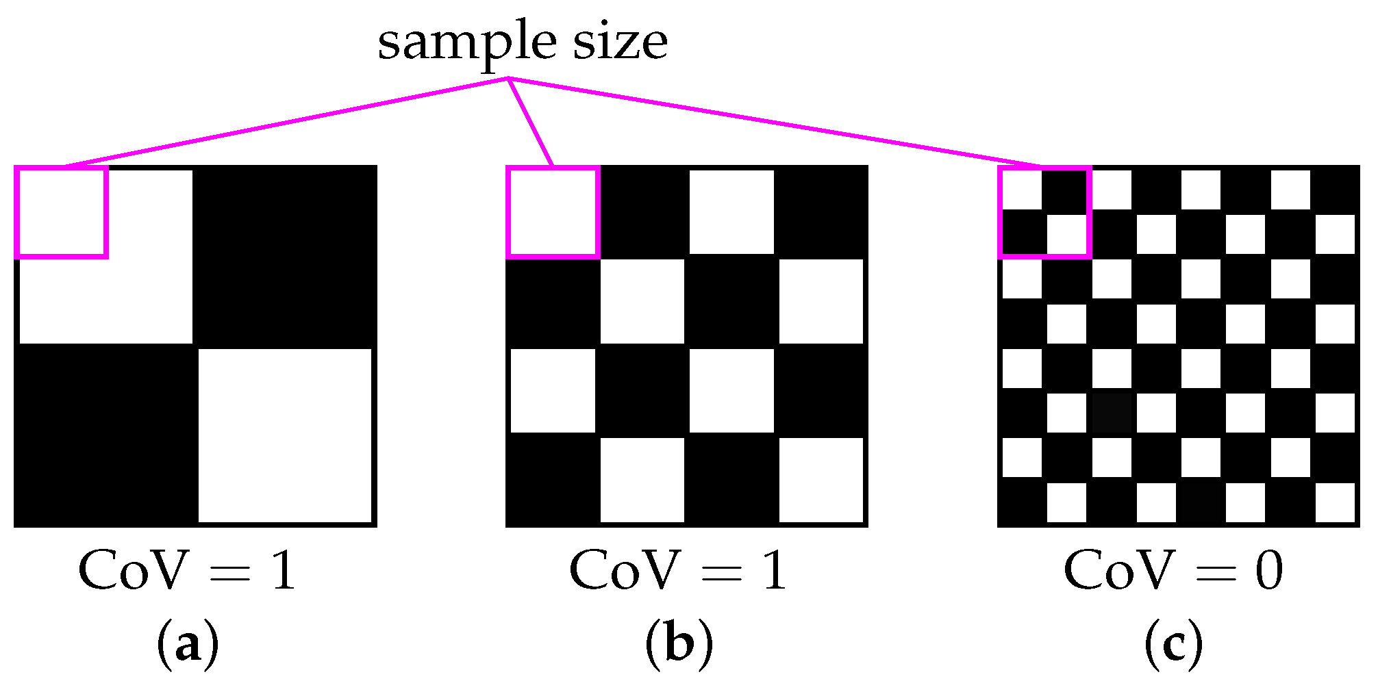
In experiments, the smallest possible scale of scrutiny (sample size) is limited by the smallest retrievable probe, such as the pixel size of a camera or the volume of a pipette. Below this threshold, concentration differences within a probe or pixel are averaged. In CFD simulations, the minimum sample size is typically constrained by the mesh resolution, especially in multiphase flow analysis. However, in single-phase flows, the sample size can be independently defined by tracking particles through the CFD-computed flow field, irrespective of mesh size. To evaluate particle concentration distributions, samples must be chosen such that they do not overlap and contain a sufficiently large number of particles (i.e., number of samples ≪ number of particles). On average, at least 10 particles per sample are recommended to ensure statistically meaningful results [71]. The sample size significantly influences statistical mixing metrics based on variance or standard deviation [32,33,41,71,85,86,87,88]. Smaller sample sizes resolve local (concentration) differences more accurately, which typically results in lower calculated mixing quality [71,89] (see Figure 6).
Since statistical mixing indices are affected by sample size, it is essential to report the resolution used. Reported resolutions vary considerably, which limits comparisons between studies unless it is confirmed that the mixing index value is independent of resolution. In some cases, the index stabilizes beyond a certain resolution [90]. Examples of used resolutions include 10 × 10 [30], 16 × 16 [90], 64 × 64 [65,91], 70 × 70 [54], 200 × 200 [86], and 640 × 480 [89].
In some experiments, only 4 [92] or 9 [38] samples are taken, which do not cover the entire cross-section; thus, both their number and spatial placement affect the mixing quality measures [71]. At least one sample should represent the least-mixed region to provide a representative measure, which requires prior process knowledge [71].
(a)
Variance and Standard Deviation
Many mixing quality measures are based on the variance σ a 2 or the standard deviation σ a of the probability density function f ( a ) of concentration a, as illustrated in Figure 5 [33]. The variance is calculated using Equation (9) [31,33].
σ a 2 = ( a i a ¯ ) 2 ¯ = i = 1 N ( a i a ¯ ) 2 N = a i 2 ¯ a ¯ 2 = i = 1 N a i 2 N a ¯ 2
If the mean concentration a ¯ is unknown and estimated from local sample concentrations a i or from flow rates V ˙ A and V ˙ B according to Equation (10) [13,32], the estimated variance σ a , est 2 is calculated using Equation (11) [32].
a ¯ est = i = 1 N a i N = V ˙ A V ˙ A + V ˙ B
σ a , est 2 = i = 1 N ( a i a ¯ est ) 2 N 1
Assuming a completely segregated state (maximum variance), the concentration a 0 j only takes values 0 or 1. For a mean concentration a ¯ , the fraction of fluid A with a 0 j = 1 is a ¯ N 0 , and for fluid B with a 0 j = 0 it is N 0 ( 1 a ¯ ) . The variance of a fully segregated system σ 0 2 , often assumed as the inlet condition, is calculated with Equation (12).
σ 0 2 = j = 1 N 0 ( a 0 j a ¯ ) 2 N 0 = a ¯ ( 1 a ¯ )
For a fully homogeneous mixture, the variance approaches zero [33]. However, only stochastic homogeneity σ z 2 can be achieved in practice [33]. For a binary mixture of fluids with equal density, it is given by Equation (13) [33]:
σ z 2 = a ¯ ( 1 a ¯ ) v ¯ V s = σ 0 2 v ¯ V s
where a ¯ denotes the mean concentration of fluid A, v ¯ is the molecular volume and V s the sample volume (analogous to Danckwerts’ scale of scrutiny). For a fully segregated system, the initial standard deviation σ 0 is given by Equation (14).
σ 0 = a ¯ ( 1 a ¯ )
Stochastic homogeneity for a binary mixture with equal density yields Equation (15):
σ z = a ¯ ( 1 a ¯ ) v ¯ V s = σ 0 v ¯ V s
The mixing quality measures based on variance, standard deviation, or distribution density functions can be experimentally quantified via several concentration measurement techniques, including conductivity, color-change or decolorization reactions as well as heat release from reactions [33,82]. Among these methods are positron emission particle tracking (PEPT) [93], magnetic resonance imaging (MRI) [93,94], (planar) laser-induced fluorescence (PLIF/LIF) [95,96,97,98], particle image velocimetry (PIV) [96], cross-sectional sampling [99], and conductivity measurements such as electrical resistance tomography (ERT) [100].
For pressure-driven mixers, such as static mixers, the mixing quality measure should be flux-weighted since the mixing in cross sectional areas with high axial velocity and thus high local volumetric flow rate is more relevant than mixing close to the walls with low axial velocity [101]. One methodology for achieving this is to select the size of the sample areas in such a way that the product of the local areas and the local axial velocities is equal [13]. Alternatively, for areas of equal size, the concentrations of the samples can be weighted with axial velocities or volumetric flow rates [13,86,93]. To calculate the flux-weighted variance σ F a 2 the local concentrations a i are weighted by the local volumetric flow rates of the areas V ˙ i relative to the volumetric flow rate of the mixer V ˙ [86,93], as shown in Equation (16).
σ F a 2 = 1 V ˙ i = 1 N ( a i a ¯ ) 2 V ˙ i
In a similar way, the volume flux-weighted standard deviation σ F a can be obtained. The flux-weighted quantities can then be used to determine mixing quality measures. The advantage of this method is that it takes into account the residence time distribution [101].
(b)
Intensity of Segregation
Danckwerts defines the intensity of segregation I for a binary mixture of fluids A and B in terms of the mean concentration a ¯ and the local concentrations a i of fluid A according to Equation (17) [31]:
I = σ a 2 σ 0 2 = ( a i a ¯ ) 2 ¯ a ¯ ( 1 a ¯ ) = i = 1 N ( a i a ¯ ) 2 N a ¯ ( 1 a ¯ )
I = 1 corresponds to complete segregation, while I = 0 indicates perfect homogeneity. I quantifies the deviation of local concentrations from the mean, but provides no information on the spatial distribution or the microstructure of the mixture. For example, I remains constant even if the size and shape of segregated regions change due to stretching, shifting, or splitting-processes that visually improve the mixture. In such cases, improvements can only be captured by dispersive mixing criteria such as the scale of segregation [34,35].
(c)
Coefficient of Variation and Relative Standard Deviation
Statistical measures such as the coefficient of variation (CoV) and the relative standard deviation (RSD) are widely used for quantitative assessment of mixing quality in many industrial applications. In this context, the coefficient of variation (CoV) is calculated from the standard deviation σ a and the mean concentration a ¯ with Equation (18) [34,39]:
CoV = σ a a ¯ = 1 N i = 1 N a i a ¯ a ¯ 2
When a ¯ is estimated from the measured concentrations a i as a est ¯ = 1 N i = 1 N a i , and σ a , est is used accordingly, cf. Equations (10) and (11), the CoV is calculated with Equation (19) [13,40]:
CoV = σ a , est a est ¯ = 1 N 1 i = 1 N a i a est ¯ a est ¯ 2
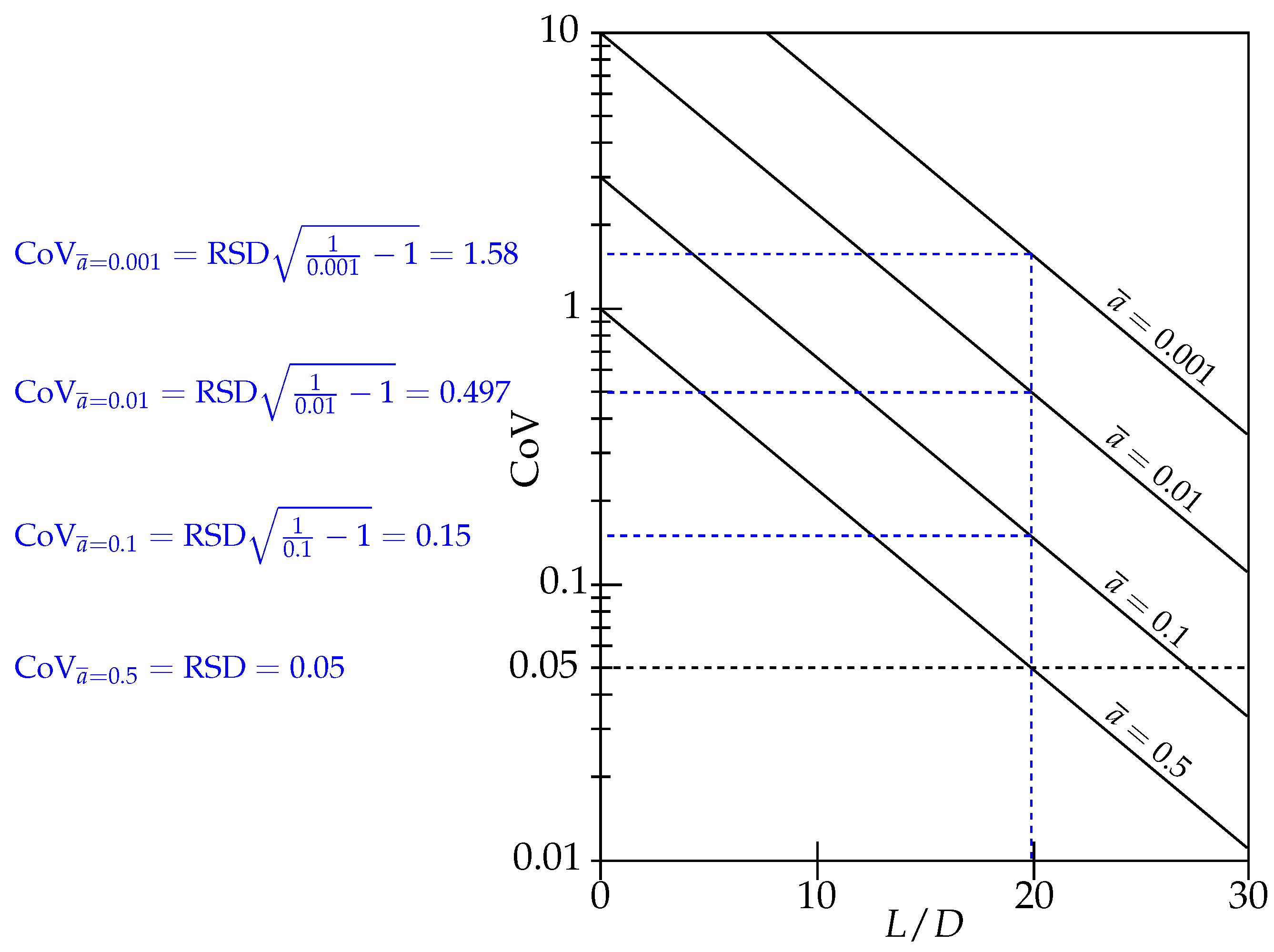
In industrial applications, a mixture is typically considered sufficiently homogeneous if CoV 0.05 [36,37,40]. In more sensitive cases, such as color mixing, even lower values may be required, e.g., CoV < 0.01 [13]. The CoV depends on the composition ratio of fluids A and B. At constant mixing intensity, CoV increases with increasing imbalance between fluid fractions (i.e., a ¯ 0 with 0 < a ¯ 0.5 ), indicating reduced mixing efficiency (see Figure 7).
To account for varying initial concentrations a ¯ , CoV can be normalized by its inlet value CoV 0 = σ 0 / a ¯ , yielding the relative standard deviation (RSD) shown in Equation (20) [13,34]:
RSD = CoV CoV 0 = σ a σ 0 = CoV 1 a ¯ 1
CoV, RSD, and the intensity of segregation I are interrelated according to Equation (21):
RSD = σ a a ¯ ( 1 a ¯ ) = CoV 1 a ¯ 1 = I
For a given RSD and arbitrary a ¯ , the CoV can be obtained via Equation (22):
CoV a ¯ = RSD 1 a ¯ 1
At equal volume fractions ( a ¯ = 0.5 ), it follows that CoV a ¯ = 0.5 = RSD .
(d)
Absolute Deviation Measures for Qualitative Assessment
In addition to variance- and standard deviation-based approaches for evaluating mixing quality, such as the CoV, RSD or the intensity of segregation, absolute deviation measures can also be used to characterize the homogeneity of a mixture. These measures are particularly useful when technical or regulatory requirements impose limits on the maximum allowable concentration deviation [23]. They allow for a direct assessment of how much individual local concentrations deviate from the mean value, an aspect that can be critical in reactive mixtures, pharmaceutical formulations, or color systems. Furthermore, they are intuitive and can be directly compared to defined limit values.
The maximum absolute relative concentration deviation δ max [82] is calculated with Equation (23) based on the difference between the smallest or largest concentration value, a min or a max , depending on which deviates more from the mean concentration a ¯ . For a symmetric distribution function, this deviation is defined as Δ a max = a max a ¯ = a ¯ a min [82]; see Figure 5a. This measure is often applied when a maximum deviation from the target concentration must not be exceeded [23].
δ max = Δ a max a ¯
The mean absolute relative deviation δ ¯ is obtained by integrating (or summing) all deviations Δ a between the concentration frequency distribution f ( a ) and the mean concentration a ¯ [82] as shown in Equation (24).
δ ¯ = Δ a ¯ a ¯ = 1 a ¯ 0 1 Δ a f ( a ) d a = 1 a ¯ 0 1 | a a ¯ | f ( a ) d a 1 a ¯ i = 1 N | a i a ¯ | N = 1 a ¯ i = 1 N ( a i a ¯ ) 2 N
The degree of deviation Δ , introduced by Käppel [33] and given in Equation (25), relates the mean absolute concentration deviation Δ a ¯ to its value before mixing, Δ a 0 ¯ [33,82].
Δ = Δ a ¯ Δ a 0 ¯ = 0 1 ( a a ¯ ) f ( a ) d a 2 a ¯ ( 1 a ¯ ) = a ¯ 1 ( a a ¯ ) f ( a ) d a a ¯ ( 1 a ¯ )
The degree of deviation can be measured directly in decolorization experiments under the assumption of chemical equivalence between a dye and a decolorizing agent [33]. Käppel developed a universally applicable decolorization experiment method that combines low experimental effort with high measurement accuracy [33]. This method determines Δ independently of sample size, does not interfere with the flow, enables continuous measurements during the mixing process, and evaluates the entire mixed material when using multiple sensors or a movable measurement device. Furthermore, the test fluid can be reused [33].
(e)
Mixing Index
An alternative way to express the described measures for distributive mixing is via the mixing index M. This index equals 0 (0%) for a completely unmixed system and 1 (100%) for a fully homogeneous mixture [82,102,103,104]. The mixing index is defined relative to various mixing quality measures, such as RSD, CoV / CoV 0 , I, CoV, or the quantities δ max , δ ¯ , and Δ ; see Equations (26) to (31). Therefore, the reference measure must be explicitly stated to ensure comparability between different publications [82]. When the mixing index is defined in terms of δ max , δ ¯ , or CoV, M approaches 1 as mixing improves. However, unlike definitions based on CoV / CoV 0 , I, and Δ , M does not necessarily equal 0 for a completely unmixed state at arbitrary values of the mean concentration a ¯ [82].
M RSD = 1 RSD = 1 CoV CoV 0 = 1 σ a σ 0 = 1 I = M I
M I = 1 I = 1 σ a 2 σ 0 2
M Δ = 1 Δ
M CoV = 1 CoV
M δ max = 1 δ max
M δ ¯ = 1 δ ¯
There are further metrics for assessing concentration homogeneity. These are also primarily based on quantities such as σ a 2 , σ a , σ 0 2 , σ 0 , σ z 2 , σ z , a ¯ , and Δ a , but they relate these variables in ways that differ from the measures presented here. Some of these additional indices are listed in [33,87].
(f)
Describing Size of Segregated Regions Using Distributive Mixing Measures
If a sample size is defined and the concentration values within this sample are averaged, distributive mixing quality measures based on variance or standard deviation can be applied accordingly. This discretization through sampling can be purposefully employed to describe a mixture solely using statistical mixing indices [86]. In order for the variance to decrease from 1 (complete segregation) to 0 (perfect homogeneity), two conditions must be met. First, regions of differing concentration (e.g., layers) must be smaller than the sample size. Second, the average concentration within each sample must be identical across all samples. This implies that the volume fractions of fluid A and B must be uniformly distributed across the mixer volume or cross-section and present in equal proportions in each sample. This concept is exemplified by Figure 5b and Figure 8.
As long as regions of differing concentration are larger than the sample size, the variance remains approximately 1, regardless of their spatial distribution in the mixer (coarse grained mixture). Therefore, a decreasing variance indicates that the regions of differing concentration are both smaller than the sample size and uniformly distributed throughout the mixer. However, the shape or distribution of these regions within each sample cannot be determined and would require other mixing indices that account for domain size or geometry. Still, in many industrial applications, knowing whether regions are smaller than a defined sample size and homogeneously distributed is sufficient for evaluating mixing quality. Consequently, many authors use mixing quality measures based on variance or standard deviation, which describe the differences in concentration between domains, as their primary or sole metric [36,38,86,89,92,102,105,106,107,108,109,110,111,112,113,114,115].

2.2.4. Dispersive Mixing—Describing Size and Structure of Segregated Regions

Dispersive mixing describes the process of reducing the size of particle or droplet agglomerates or gas bubbles [2,30,40,55]. Dispersive mixing metrics are especially relevant in laminar flow with low diffusion, where a clear separation between regions of different concentrations exists. In some cases, these measures are only quantifiable under such conditions.
The following metrics are used to characterize dispersive mixing.
(a)
Striation Law, Number of Striations and Interfacial Stretch
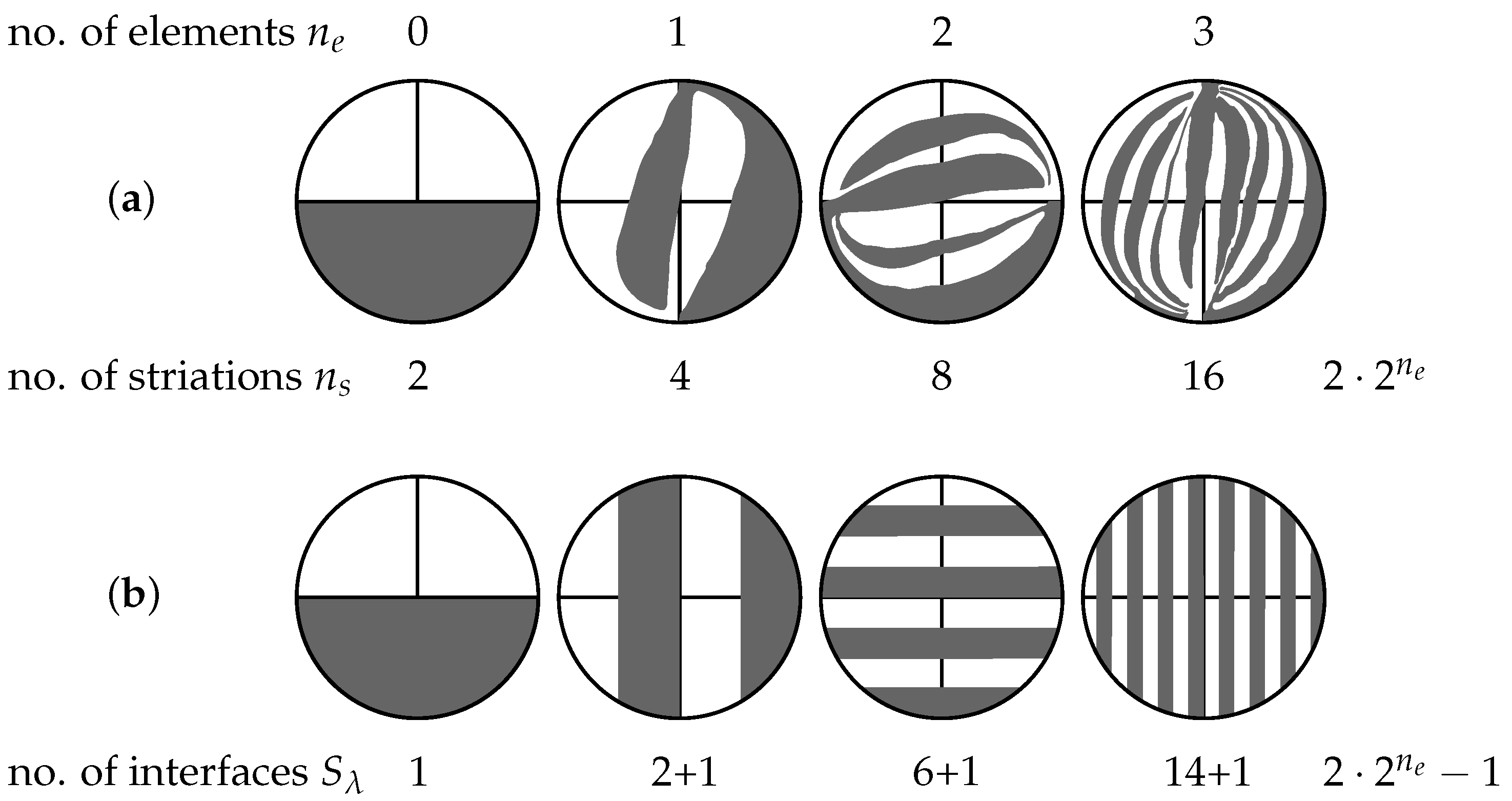
Striation laws theoretically estimate the number of striations n s formed after n e mixing elements, each with n c flow channels, under laminar conditions. Assuming k input components, a simple exponential relation can be derived [23,116] as shown in Equation (32):
n s = k · n c n e
Although useful for understanding mixing progression, this law is only an approximation and may deviate from experimental results, depending on the mixer geometry [23,117]. The striation law (32) neglects the significant influence of the volume flow ratio and is based on the simplified assumption that all layers have the same thickness, which does not apply under real operating conditions [117]. Meijer et al. [101] propose an analogue concept of the so-called interfacial stretch S λ , which is defined as the number of distinct interfaces formed relative to the initial configuration.
(b)
Scale of Segregation
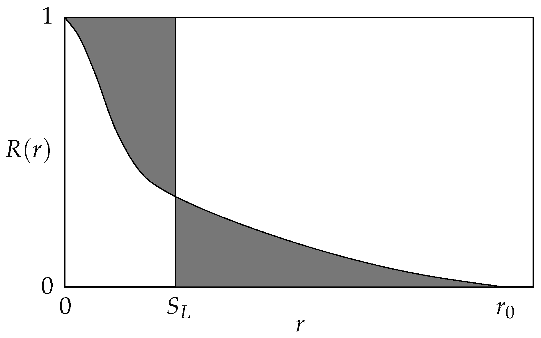
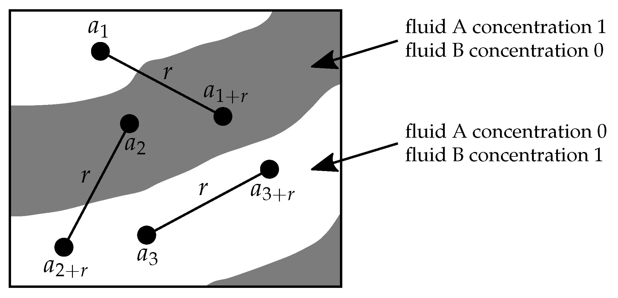
The scale of segregation, introduced by Danckwerts [31], is based on the correlation coefficient R ( r ) , also known as the autocorrelation function given by Equation (33) [31,35]. It measures the statistical dependence between a concentration value a i at position i and another a i + r at a distance r (see Figure 9). The average product of their deviations from the mean a ¯ is normalized by the concentration variance σ a 2 :
R ( r ) = ( a i a ¯ ) ( a i + r a ¯ ) ¯ σ a 2 = 1 N i = 1 N ( a i a ¯ ) ( a i + r a ¯ ) 1 N i = 1 N ( a i a ¯ ) 2
R ( r ) ranges from 1 to 1 , indicating strong positive correlation, no correlation, or inverse correlation, respectively. Negative values may arise from periodic structures in the mixture [31,35]. The graph of R ( r ) versus r is called a correlogram (see Figure 10). The distance at which R ( r ) first crosses zero, denoted r 0 , defines the correlation length [35,41], i.e., the scale below which domains can be considered statistically homogeneous.
Danckwerts defined the linear scale S L as the integral of R ( r ) according to Equation (34) [31]:
S L = 0 R ( r ) d r = 0 r 0 R ( r ) d r
and the volume scale S V given by Equation (35) [31]:
S V = 2 π 0 r 2 R ( r ) d r = 2 π 0 r 0 r 2 R ( r ) d r
In practice, R ( r ) is often computed at discrete distances. For approximating S L or S V , numerical integration (e.g., trapezoidal rule or curve fitting) is used. If R ( r ) slowly decays to zero, identifying r 0 directly or via a threshold (e.g., R ( r ) < 2 / N for 95% confidence) is often more reliable [35,41]. Using the striation law (32), the theoretical scale of segregation S L can be estimated in relation to the scale of segregation at the mixer inlet S L 0 according to Equation (36) [118].
S L = D n s = k · S L 0 n s = S L 0 n c n e
(c)
Interfacial Area
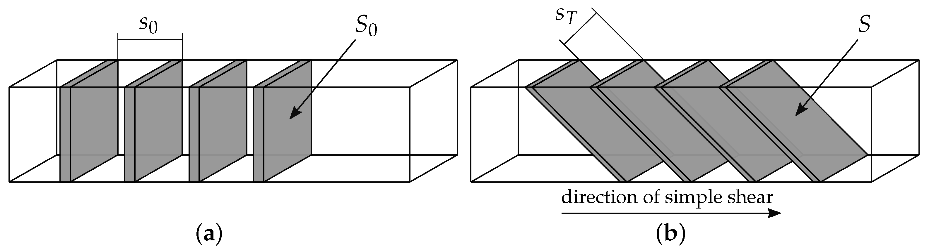
The interfacial area provides a quantitative measure of the surface formed between two fluids during laminar mixing, especially relevant in highly viscous systems where turbulence and diffusion are negligible. The concept of interfacial area was introduced by Spencer & Wiley [43]. It quantifies the surface area S formed between two fluids as a function of the initial interface S 0 , shear, and the alignment between the interface and shear direction. Under simple (unidirectional) shear and a flat interface, the interfacial area can be calculated using Equation (37) [42,43] (for simple shear u y y = u z y = 0 ):
S = S 0 1 2 u x y cos α x cos α y + u x y 2 cos 2 α x
For curved interfaces and multidirectional shear, local shear and orientation relative to the interface must be considered. The average radius of curvature must significantly exceed half the resolution limit for meaningful quantification [43]. Although the interfacial area reflects the dispersion of concentration regions, it does not provide information about their spatial distribution [43].
(d)
Striation Thickness and Striation Thinning
The concept of striation thickness was derived by Mohr et al. [42] from the interfacial area Equation (37). It is therefore also based solely on shear and is suitable for evaluating laminar mixing processes of highly viscous fluids. The striation thickness depends on the interfacial area according to Equation (38), with a factor of 2 because all striations, except the two adjacent to the walls, have two interfaces [42]. The striation thickness s T is defined according to Equation (38):
s T 2 V S
with the total interfacial area S and the total volume of the system V. Alternatively, the striation thickness can be defined as the ratio of the area A eq . c to the perimeter L eq . c of regions with equal fluid composition or concentration in a cross-sectional plane, e.g., at the inlet or outlet according to Equation (39) [46,47,48]:
s T = A eq . c L eq . c
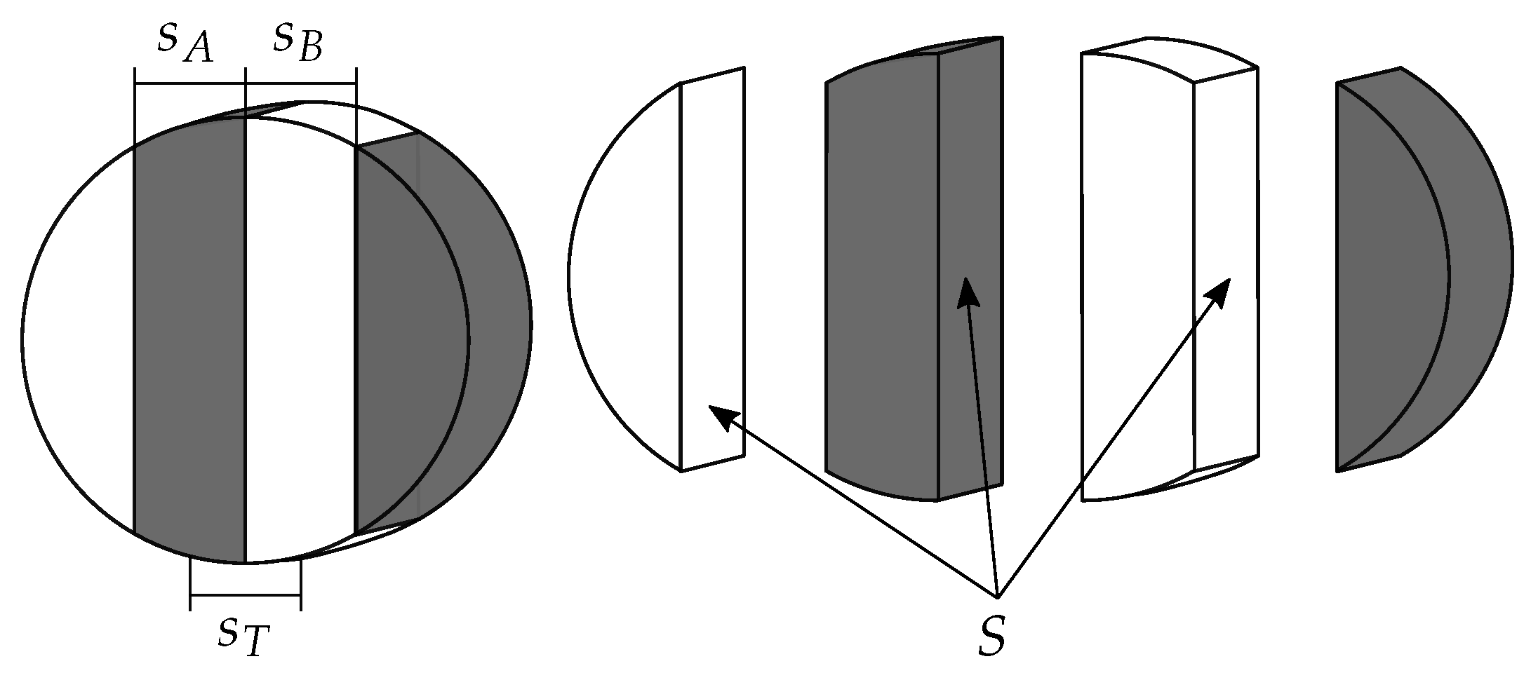
For an ideal laminar structure with constant layer thicknesses, the striation thickness can also be approximated by the average of the layer thicknesses s A of fluid A and s B of fluid B, as shown in Equation (40) (see Figure 11) [44]:
s T = s A + s B 2
In the case of simple (unidirectional) shear and a flat interface, the striation thickness can also be calculated using the following Equation (41) [42]:
s T = s 0 V ϵ B V A μ A μ B
with initial striation thickness (side length of cubes of the minor component) s 0 , shear strain on the major component (product of shear rate imposed on major component and residence time) ϵ B , volume of the minor component V A , viscosity of the major component μ B and viscosity of the minor component μ A . If μ A / μ B < 1 , the viscosity ratio is set to 1, since the minor component cannot deform faster than the major component matrix [42].
Under simple shear perpendicular to the initial striations, the striation thickness decreases and the interfacial area increases (see Figure 12). However, the reduction in striation thickness diminishes over time, as the striations align with the direction of shear. A more efficient thinning is achieved if the shear direction changes periodically so that it remains perpendicular to the striations [13].
The probability density function of the different striation thicknesses in the spatial structure of the partially mixed fluids is referred to as the striation thickness distribution [45]. Employing the striation law (32), the theoretical striation thickness s T can be estimated in terms of the striation thickness at the mixer inlet s 0 by means of Equation (42) [22,117].
s T = D n s = k · s 0 n s = s 0 n c n e
The striation thinning α s describes the temporal change in striation thickness (e.g., between the inlet and outlet of the mixer) [46,48]. It is calculated with Equation (43) and analogous to the stretching function α λ defined by Ottino in Equation (48) [50].
α s ( t ) = d ln ( s T ) d t
Integration for a constant value of α s leads to Equation (44), as derived by Fourcade et al. [46,48,49].
α s = 1 t ¯ ln s T s 0 = L c ¯ ln s T s 0
The striation thickness can be investigated experimentally using LIF (Laser-Induced Fluorescence) systems [119]. It can also be determined from CFD simulations using particle tracking methods, in which particles are introduced at the inlet within a small circular area (corresponding to s 0 ), and their distribution at the outlet or across various cross-sections along the mixer is evaluated ( s T ) [48]. However, determining striation thickness experimentally is challenging, and CFD calculations can be affected by numerical diffusion and sampling issues [13].
(e)
Stretching
The determination of striation thickness (and interfacial area) is often complex, as it requires resolving the actual spatial structures that form during the mixing process [45]. A more straightforward approach is to determine the stretching of a number of points distributed throughout the entire flow field, which is closely related to both the striation thickness and interfacial area [45]. The increase in interfacial area S per unit volume V is proportional, and the striation thickness s T is inversely proportional to the stretching (also referred to as stretch ratio or accumulated stretching) λ [46,54] as shown in Equation (45):
λ S V 1 s T
In general, higher stretching rates indicate better mixing or micromixing quality [65,66]. Therefore, the stretching rate is widely used as an indicator for estimating micromixing quality [66]. To determine the stretching rates λ , the change in length | d x | of small vectors attached to fluid particles moving with the flow (e.g., 100 vectors per particle uniformly distributed in direction [45]) is compared to their initial length | d X | [54]. The stretching is then calculated according to Equation (46) [1,30,44,54,60,61].
λ = lim | d X | 0 | d x | | d X |
The stretching rate λ can be directly computed from the deformation tensor F and the initial material orientation M using Equation (47) [1,63]:
λ = ( F · F T ) : M M 1 / 2
Here, F is the deformation tensor F = x i / X j , with d x ( t ) = F ( t ) · d X , and M d X / | d X | denotes the initial material orientation.
The instantaneous stretching rate, or stretching function, as introduced by Ottino [50], is defined in Equation (48) [1,50]:
α λ = D ( ln λ ) D t = D : mm
Here, D ( ) / D t denotes the material derivative, m d x / | d x | is the instantaneous orientation, and D = 1 2 [ v + ( v ) T ] is the rate-of-deformation tensor.
If the time-averaged stretching function is constant and positive, the flow efficiently mixes material elements regardless of their initial position or orientation [1,62]. However, since both the instantaneous and averaged values depend on the time scale, the stretching function is not suited for comparing different flow fields [1]. Instead, the (frame-invariant [39]) stretching efficiency e λ provides a more appropriate metric [1,39,50,63]. It is calculated using Equation (49).
e λ = D ( ln λ ) / D t ( D : D ) 1 / 2 1
The closer e λ is to 1, the more effective the flow is at generating stretching [1].
As a symmetric tensor, D has three orthogonal eigenvectors n 1 , n 2 , and n 3 associated with eigenvalues λ 1 > λ 2 > λ 3 [1,39,67]. Maximum and minimum specific stretching rates occur in the directions of n 1 and n 3 , respectively. The corresponding maximum stretching efficiency is given by Equation (50) [1,39,67]:
e λ , max = λ 1 ( D : D ) 1 / 2
For axisymmetric extensional flows, e λ , max = 2 / 3 0.816 ; for squeezing flows, e λ , max = 1 / 6 0.408 ; and for two-dimensional flows such as simple shear, e λ , max = 1 / 2 0.707 [1,39,50,67].
Please note that among the various dispersive mixing measures, stretching plays a central role. It is fundamentally a deformation-based quantity, derived from the local deformation tensor of infinitesimal fluid elements. At the same time, stretching provides direct insight into the chaotic nature of the flow, as quantified by the Lyapunov exponent, and serves as a basis for other scale-dependent measures, such as striation thickness and interfacial area. Consequently, while classified as deformation-based in the Introduction, stretching simultaneously captures aspects of flow chaos and scale-related phenomena, highlighting its multifunctional significance in characterizing dispersive mixing in static mixers.
(f)
Lyapunov Exponent
In the early 1990s, laminar mixing was analyzed using tools from chaos theory [50,62,64]. The Lyapunov exponent δ characterizes the degree of chaos and serves as an indicator of mixing efficiency. It relates to the stretching rate λ and is conceptually defined as stretching per unit time and is calculated with Equation (51) [46,60]:
δ = lim t log ( λ ) t
In steady flows through static mixers with n e elements, the Lyapunov exponent can be approximated by Equation (52), where t e is the residence time per element [61].
δ = lim n e 1 n e t e i = 0 n e 1 ln ( λ i )
To ensure independence from the initial segment length, λ is evaluated for infinitesimal vectors | d X | 0 [61]. The Lyapunov exponent thus represents the long-term average of the instantaneous stretching rate Equation (48) [50], and the stretching efficiency Equation (49) can be interpreted as a normalized Lyapunov exponent.
A positive Lyapunov exponent implies exponential growth in λ , which corresponds to exponential increase in interfacial area S and thinning of striations s T [46]; see Equations (38) and (45). Higher values of δ indicate more chaotic systems and, in principle, improved mixing quality [60].
To determine λ and δ , tracer particles with attached stretch vectors are tracked through the mixer. Their positions and vector lengths are recorded after each element to calculate λ and δ [46]. For global mixing evaluation, the spatial distribution or probability density function of Lyapunov exponents from multiple initial positions can be analyzed [63]. Note that both the stretching rate and the Lyapunov exponent represent upper bounds for the striation thinning rate α s , as α s is typically evaluated neglecting stretching in the primary flow direction [46].
(g)
Extensional Efficiency
The extensional efficiency, introduced by Manas-Zloczower [69], is a key parameter in evaluating dispersive mixing [2]. However, it should be considered alongside the magnitude of shear stresses in the flow field [69].
Extensional efficiency e α is defined in Equation (53) based on the rate-of-deformation tensor D = 1 2 v + ( v ) T and the vorticity (spin) tensor Ω = 1 2 v ( v ) T [13,30,40,55,61,68]:
e α = | D | | D | + | Ω |
Characteristic values of the extensional efficiency are:
  • e α = 1 for pure extension,
  • e α = 0.5 for simple shear,
  • e α = 0 for pure rotation [13,40,61,68,69].
Extensional flows (converging and diverging particle motion) have been shown to be more effective for dispersive mixing than simple shear flows (sliding motion) [60,69]. Hence, higher e α values suggest better dispersion performance [40,68].
In static mixers, e α typically ranges between 0.5 and 1, though it may vary significantly along the flow path [13,30]. Note that e α is not frame-invariant and thus not objective in the rheological sense [60,61]. However, it remains suitable for comparing static mixers when the analysis is based on the same Eulerian reference frame [60]. Moreover, e α is not a direct measure of overall mixing quality, as it does not account for particle segregation [60,61,68]. Nonetheless, it provides a meaningful metric for characterizing macro-mixing behavior [66].
(h)
Shear Rate
In laminar flows, extensional efficiency and stretching are independent of the flow rate. However, the dispersive capacity of a mixer is depending on the flow rate [30]. Consequently, extensional efficiency and stretching are not sufficient as quality measures in this case. Flow rate-dependent quantities such as the shear rate γ ˙ or mean shear rate γ ˙ ¯ can be used as indicators of a mixer’s dispersion capacity, i.e., the capacity to break up droplets and bubbles [61]. The shear rate γ ˙ is derived from the rate-of-deformation tensor D using Equation (54) [39].
γ ˙ = 2 ( D : D )
The shear rate is dependent on the pressure drop, and thus provides information about the degree of shear. To understand the relationship between energy loss and input conditions, a more appropriate interpretation should be made based on the conversion of the pressure drop to shear [61].

2.2.5. Exposure

In certain applications, such as reactions, both the size of areas of equal concentration (scale of segregation) and the intensity of the differences between these areas (intensity of segregation) influence the mixing and reaction process. In such cases, it is advisable to consider these measures in combination. Exposure is defined as this combination and describes the potential or the rate of change of differences in concentration. It depends nonlinearly on the intensity of segregation and the scale of segregation [34]. A simple definition of exposure is the interface area multiplied by the concentration difference between the areas [34]. Parameters that depend on exposure and can thus be used for its evaluation include mass transfer or molecular diffusion, heat transfer or reaction rate, and droplet breakup or coalescence rate. [34].
For various mixing applications, different mixing quality measures are dominant (D) or relevant (R) indicators of good mixing as well as rapid reactions; see Table 1 [34].
In the context of miscible fluids, the dominant and relevant indicators are contingent on the prevailing flow regime and the nature of the fluid (Newtonian or non-Newtonian). The intensity of segregation is the dominant mixing quality measure for turbulent flows, and the scale of segregation is the dominant measure for laminar mixtures. However, the intensity of segregation can also be used to determine whether areas of equal concentration are smaller than a specified sample size and at the same time homogeneously distributed, as described in the section on distributive mixing measures. Therefore, it can be used to make a combined assessment of scale and intensity of segregation within the meso scale. For this reason it is considered the sole mixing quality measure in many industrial applications involving miscible fluids. In the context of multiphase flows of immiscible fluids, the dominance and relevance of different mixing quality measures depend on the specific mixing step. The initial step is the interruption of the separation of the fluids at the macro scale by splitting them into smaller areas. The scale of segregation can be used as a mixing quality measure for this purpose. In the second step, the areas are distributed homogeneously within each other. For this purpose, the intensity of segregation in the meso scale (where the sample size is significantly larger than individual particles, bubbles, drops) can be considered. In the third step, the distributed meso scale areas are continuously reduced to the micro scale. In this context, the scale of segregation is the dominant measure. The final step in the mixing of several phases is mass transfer (diffusion) or the dissolution of the smallest particles. In this case, exposure is the dominant mixing measure, as these processes depend on both the size of the smallest areas and the concentration differences.
The same applies to mixing-sensitive reactions with an order other than 1. The order of a reaction describes the degree to which the reaction rate depends on the concentrations of the reactants. Reactions with an order greater than 1 have a higher reaction rate if the scale of segregation of the areas with equal concentration is small and there is a high concentration gradient, i.e., a high intensity of segregation at the boundaries of the areas [31]. Reactions with an order less than 1 have a higher reaction rate at small concentration gradients, and reactions with an order equal to 1 are independent of concentration [120].

2.3. Correlations of Mixing Quality Measures for Static Mixers

The following section provides an overview of the correlations available for assessing the mixing quality measures in static mixers.

2.3.1. Element Number for Homogenization

The first descriptions and applications of static mixers focused on the number of mixing elements required for “homogeneous mixing”, although it was usually not defined quantitatively. The number of Kenics elements required for homogenization can be described using Equation (55), which was determined by means of a decolorization reaction [121].
n e = C 1 · Re E 1 · Sc E 2 V ˙ B V ˙ A E 3 μ 1 μ 2 E 4
The parameter C 1 and the exponents E 1 , E 2 , E 3 and E 4 depend on the Reynolds and Schmidt numbers as well as on the viscosity ratio and volume flow ratio of the mixed fluids [121]; they are listed for the Kenics mixer in [121]. The impact of the Reynolds number on the number of elements required for homogenization is noteworthy. The number of Kenics elements required to obtain a homogeneous mixture remains constant for Re < 1 and then rises slowly at first. As the value of Re increases from approximately 10, the number of elements required increases sharply and reaches a maximum at Re 50 . Thereafter the number of elements decreases and reaches a minimum, whereupon it remains approximately constant for Re > 2000 [13,116,121]. This finding, together with other studies on pressure loss, suggests that the flow within a Kenics mixer remains laminar up to a Reynolds number of approximately 50, followed by a transition regime. Beyond a Reynolds number of approximately 2000, the flow becomes fully turbulent [121]. However, this effect is not apparent in other scientific contributions and manufacturer’s specifications, such as those shown in Table 2.
As can be seen in the manufacturer’s specifications in Table 3, the number of mixing elements n e required to obtain a homogeneous mixture is also influenced by the maximum viscosity μ 1 and the minimum viscosity μ 2 of the fluids as well as the ratio μ 1 / μ 2 .

2.3.2. Residence Time

The mean residence time t ¯ in the Kenics mixer can be calculated using Equation (56) [59].
t ¯ = 2 · D · L E D · n e · 0.68 + 0.22 · c ¯ 1.03

2.3.3. Intensity of Segregation, Coefficient of Variation

The coefficient of variation CoV generally depends on the following parameters.
  • Relative mixer length L / D [122];
  • Aspect ratio L E / D [122];
  • Relative hydraulic diameter d h / D [122];
  • Volume flow ratio; V ˙ A / V ˙ B [122];
  • Viscosity ratio μ A / μ B [122];
  • Rheology (Newtonian or non-Newtonian fluids) [123];
  • Reynolds number Re [122];
  • Archimedes number Ar or density ratio ρ A / ρ B [122];
  • Schmidt number Sc [122];
  • Weber number We [122];
  • Prandtl number Pr [122].
The relative mixer length L / D specifies the number of mixing elements n e , taking into account the aspect ratio of the mixing elements L E / D as shown in Equation (57).
n e = L D D L E = L L E
The aspect ratio L E / D of an element also influences the CoV, since shorter elements, for example, initiate faster changes in direction and turbulence, which generally increases the mixing intensity and pressure loss. The aspect ratio L E / D and the relative hydraulic diameter d h / D are constant for a fixed mixing element geometry.
The volume flow ratio V ˙ A / V ˙ B strongly influences the mixing quality when it deviates from the range of 0.01 to 100 ( 0.01 < a ¯ < 0.99 ). In this case, special injectors or dynamic mixers may be required [13]. The effect of volume flow ratio can be taken into account using Equation (22).
The viscosity ratio μ A / μ B has a significant influence on the resulting mixing quality. For instance, a viscosity ratio of μ A / μ B = 10 3 requires up to twice as many mixing elements as μ A / μ B = 1 [13,122]. It is less challenging to mix a small proportion of low-viscosity fluid into a large proportion of high-viscosity fluid μ A / μ B < 1 than vice versa μ A / μ B > 1 [13]. In instances where the viscosities of the mixed fluids are greatly disparate μ A / μ B > 10 5 , the number of mixing elements required increases to such an extent that the use of dynamic mixers is a more viable option [13]. The influence of the viscosity ratio is only relevant if μ A / μ B > 100 [122].
The rheology of fluids also influences the mixing quality. The rheology of non-Newtonian fluids can be time-independent, time-dependent, and viscoelastic [123]. In time-independent fluids, viscosity decreases with increasing shear rate (pseudoplastic-shear thinning) or increases (dilatant-shear thickening) [123]. This behavior can be described using models such as the power law model, the Herschel-Bulkley model, or the Bingham model [123]. In time-dependent fluids, viscosity depends on both the shear rate and the duration of shearing. If viscosity decreases with the duration of shearing, this is referred to as thixotropic behavior; if it increases, it is referred to as negative thixotropic behavior [123]. Viscoelastic fluids exhibit both elastic and viscous behavior [123]. Investigations have demonstrated that the CoV for specific mixer types (Inliner 45, Komax, and SMX) exhibits a marginal decrease when engaging in the mixing of shear-thinning fluids as opposed to Newtonian fluids [111,113]. The extant literature contains only limited information on the (energy-efficient) mixing of non-Newtonian fluids in static mixers [123]. The majority of studies on mixing quality focus on Newtonian fluids; therefore, the description and intensification of the mixing of non-Newtonian fluids in static mixers are areas of active and future research [123].
In laminar and turbulent flows, the influence of the Reynolds number Re is negligible [122]. Some investigations of the Kenics mixer show an increase in CoV dependent on Re in the transition range [13,122]. Other investigations of the Kenics, Inliner 45, Komax, and SMX mixers also show a CoV independent of Re for creeping flows, but no increase in CoV in the transition range [2,22,111]. For higher Reynolds numbers above approximately Re = 10 100 , these studies show a decrease in CoV with increasing Reynolds number. Upon reaching turbulent range, the CoV initially decreases strongly, after which the influence of Re diminishes [22,99].
The Archimedes number Ar and the density ratio ρ A / ρ B have an influence in creeping flows Re < 1 when the buoyancy forces are dominant in relation to the viscous forces Ar / Re > 1 [122]. In turbulent flows, Ar has an influence when the flow velocity is low and the density differences are large. However, for a Froude number F r = Re 2 / Ar > 20 , the effect of buoyancy is negligible [122]. The influence of the density difference on turbulent mixing in an SMX mixer at F r < 20 was verified through simulation (see Table 4—SMX ρ A / ρ B 1 ) [114].
The influence of the Schmidt number Sc, which is a measure of diffusion, is usually negligible in turbulent flow for most industrial applications [13,122]. In cases where the Reynolds number is low, mixing is influenced by diffusion [13]. However, this influence is only relevant in well-mixed states (micromixing) [122]. Therefore, Sc can also be neglected for laminar flows in most industrial applications, when considering macro and meso mixing.
The Weber number We exerts influence solely in the context of multiphase flows, while the Prandtl number Pr affects temperature equalization processes [122]. Consequently, these parameters can be disregarded in the context of mixing miscible fluids of equal temperature.
Assuming a binary mixture of miscible Newtonian fluids of equal temperature with a small difference in viscosity ( μ A / μ B < 100 ) and density ρ A / ρ B (laminar Ar / Re < 1 , turbulent Re 2 / Ar > 20 ) within a distinct flow regime (laminar/turbulent), the behaviour of the CoV in relation to the relative mixer length L / D can be approximated using Equation (58) [13,91,114,124,125].
CoV = A · exp B L D
A and B are correlation constants for static mixers, as derived from the extant literature, are listed in Table 4. The suffix R-R to the Kenics mixer indicates that the successive mixing elements have the same direction of rotation. The standard Kenics mixer has an alternating direction of rotation (R-L). In the R-R configuration, “unmixed islands” are formed regardless of the mixing length. Consequently, the minimum achievable CoV is greater than with the standard Kenics mixer (R-L) [65,125].
The correlation constant A depends on the average concentration a ¯ respectively the volume flow ratio V ˙ A / V ˙ B and the distribution at the inlet, e.g., due to different injection types. It corresponds to the coefficient of variation at the inlet of the mixer A = CoV 0 and can be determined for different concentrations a ¯ with Equation (22). The reduction in CoV by the mixing elements is described by the correlation constant B. A higher value of B results in a faster reduction in CoV and thus superior mixing. Therefore, if the input conditions A = CoV 0 are known, the correlation constant B is sufficient to describe the reduction in CoV.
Assuming A = 1 if a ¯ = 0.5 , Equation (58) can be simplified to Equation (59) so that the relationship between RSD and L / D depends only on a parameter K. In this case, B = ln ( K ) and K = exp ( B ) .
RSD = CoV 1 a ¯ 1 = K L / D
Some mixer types deviate from the assumed exponential behavior of the mixing quality. For instance, CFD calculations of the Inliner 45 and the SMX mixer show a lower CoV after the first mixing element and, with increasing number of elements, higher CoV values in comparison to those calculated with Equation (59) [111].
The injection type influences the coefficient of variation at the inlet CoV 0 and thus the correlation constant A. For example, in case of the SMX mixer, lower CoV values are achieved with a central injection position or ring-shaped injection on the wall than with injection from one side [115].
Vortex mixers, e.g., CompaX and HEV, generate vortices in the section after the mixer, thereby obviating the necessity for multiple mixing elements in most cases. In the context of these mixers, the relative mixer length L a / D does not refer to the number of mixing elements, but rather to the length of the section after the mixer necessary for homogenization.
According to manufacturer’s specifications (Sulzer Ltd.), CoV = 0.05 of the CompaX mixer is achieved within the turbulent regime of Re > 2300 at a length after the mixer of L a / D = 3 if the viscosity ratio is μ 1 / μ 2 < 100 and the condition ρ B ρ A / ρ B < c B 2 / ( 200 ϕ ) is satisfied [132]. Where ρ B and c B are the density and velocity of the main flow and ρ A and ϕ are the density and injector diameter of the secondary flow. The mixing quality of the HEV mixer depends on the Reynolds number. In the range 1000 < Re < 9000 , the CoV decreases more rapidly with increasing Reynolds number than in the range Re > 9000 [22]. In comparison to the SMV mixer, which is also suitable for turbulent mixing, the CompaX and HEV vortex mixers have significantly shorter installation lengths and slightly higher pressure loss [132]. Compared to HEV and SMV, the CompaX requires a shorter length to achieve CoV = 0.05 [132].

2.3.4. Striation Law, Striation Thickness, Scale of Segregation and Interfacial Stretch

For a binary mixture ( k = 2 ) in a Kenics mixer with n c = 2 [22,46,118], the striation law (32) yields n s = 2 · 2 n e (see Figure 13a). The calculation of the scale of segregation of the Kenics mixer with Equation (36), has been shown to exhibit a high degree of agreement with experimental data for Re = 0.01 and an element number n e > 1 [118]. After an SMX element in creeping flow ( Re = 0.195 ), striation thickness s T / s 0 = 0.05 [46], corresponding to n c = 20 .
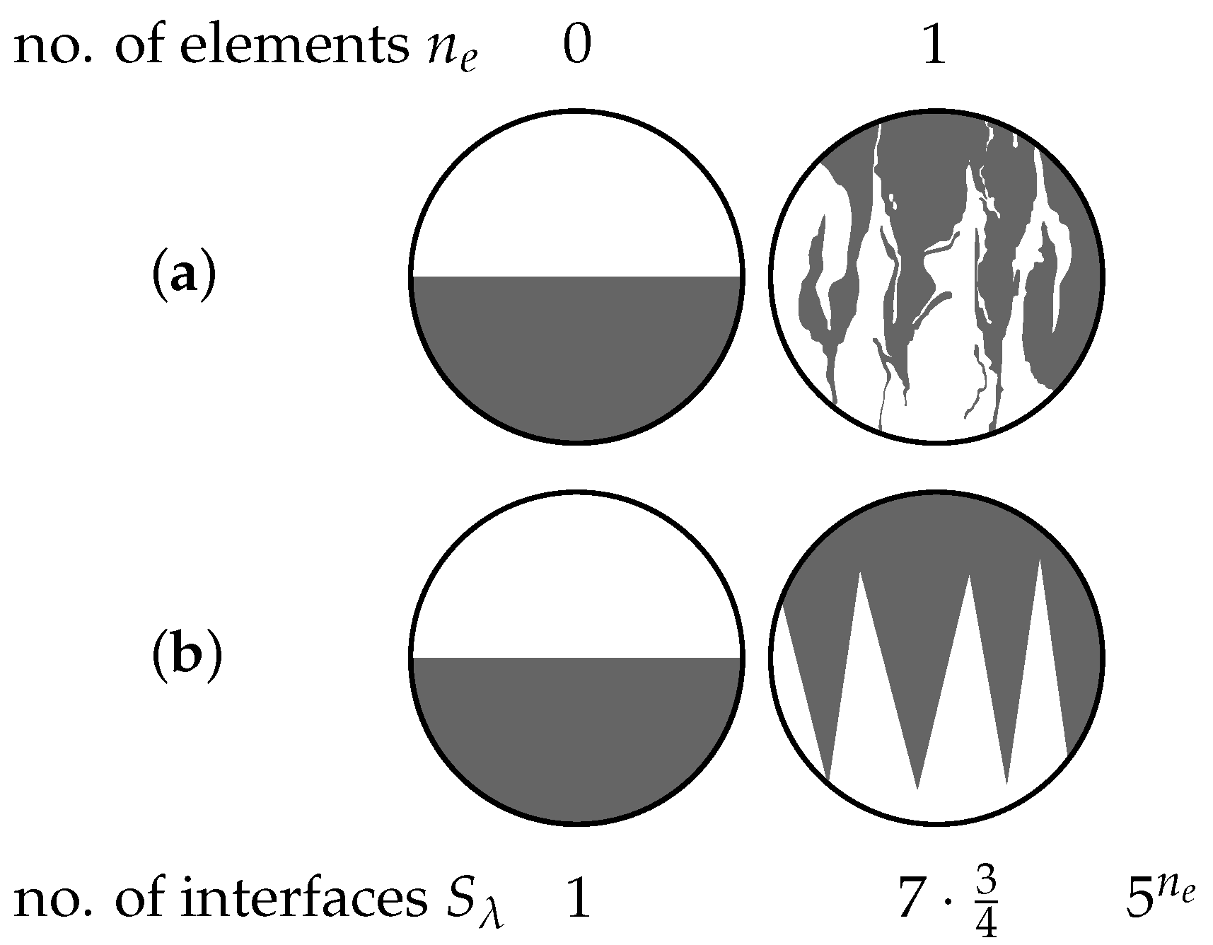
In Kenics mixers, the merging of flows after each element generates an additional interface, resulting in an approximate formula for the interfacial stretch S λ proposed by Meijer et al. [101] (see Figure 13b).
In SMX mixers uniform cross-sectional layering is not observed (see Figure 14a). Instead, about seven interfaces form per element, covering roughly 75% of the cross-section. Hence, Meijer et al. suggest an exponential estimate of 5 n e for the interfacial stretch S λ (see Figure 14b) [101].
The equations for the number of striations n s and the interfacial stretch S λ of a binary mixture in static mixers can be found in Table 5. Theoretical values of the scale of segregation S L and the striation thickness s T can be estimated from n s using Equation (36) and Equation (42), respectively.

2.3.5. Striation Thinning

Striation thinning α s is contingent on the viscosity ratio of the mixture components. As viscosity differences increase, striation thinning decreases [48]. If Re < 10 , the quotient of the mean rate of striation thinning α s and the mean flow velocity c ¯ is constant. This can be attributed to the fact that, at low Re, the streamlines are independent of the flow rate V ˙ or Re, respectively. In this instance, striation thinning is found to be linearly dependent on V ˙ or Re, respectively [49]. If Re = 0.195 , α s can be estimated at 0.02 [ s 1 ] for a single Kenics element ( L E / D = 1.5 ), and for a single SMX element, α s is approximately 0.15 [ s 1 ] [46]. The mean rate of striation thinning α s of multiple consecutive Kenics elements is higher than that of a single element and is approximately 0.03 [ s 1 ] for each of the elements [46]. In the case of Re = 5 , it was found that α s for the Kenics and Inliner 45 mixers ( L E / D = 1.5 ) is 0.14 [ s 1 ] [49].
For Re > 10 , the streamlines depend on the flow rate V ˙ , and α s is increasing nonlinearly with V ˙ or Re, respectively [49]. For higher Reynolds numbers, α s is greater in the Inliner 45 than in the Kenics mixer [49].

2.3.6. Stretching

The mean stretching λ of the Kenics mixer increases exponentially, indicating the exponential growth of separation surfaces and is a characteristic of chaotic flow [125].
The exponential growth of λ is commonly described using either log ( λ ) or ln ( λ ) [30,125], with the corresponding equation being (60).
λ = a λ · e b e L D = a λ · 10 b 10 L D
In the standard Kenics mixer with alternating rotation direction (R-L), the growth is greater than in the Kenics mixer with the same rotation direction (R-R) [125].
The mean stretching rates ln ( λ ) of three mixing elements in the laminar regime (creeping flow) are greater for SMX and ISG mixers compared to Kenics, LPD, Inliner 50, and Inliner 45 mixers (see Table 6).
In the case of Kenics, LPD, Inliner 50, and Inliner 45 mixers, the injection position is of significance, with areas in the middle of the pipe showing less stretching in comparison with areas in proximity to the walls. In the case of SMX and ISG mixers, the injector position does not affect the stretching [30].
The stretching efficiency e λ , max of the SMX mixer at laminar flow ranges between 0.4 and 0.8. Consequently, all conventional flow types are evident, namely simple shear, pure elongation, and squeezing. At e λ , max = 0.8 , the flow converges and at e λ , max = 0.4 it diverges [39]. These flows are indicative of elongational and squeezing flows in incompressible fluids [39].

2.3.7. Lyapunov Exponent

The Lyapunov exponent δ was found to be higher in the case of a central injector position in the SMX and KMX mixers than in the case of a non-central injection. This finding indicates that a central injector position results in more chaos and better mixing (it should be noted that only one non-central position was tested) [61].
The specific stretching rate α of the Kenics mixer is analogous to the Lyapunov exponent δ ( α = lim n p ln ( λ ) / n p with period n p ) [91,124]. It depends on the Reynolds number [124]. For Re < 10 and Re = 1000 , the specific stretching rate α is higher than for Re = 100 . This indicates less chaotic flow as well as mixing quality in the transition regime and is consistent with the results of the CoV [124].
The results of investigations for the Lyapunov exponent δ and the specific stretching rate α are listed in Table 7.

2.3.8. Extensional Efficiency

The extensional efficiency e α in the Kenics mixer exhibits a maximum at the inlet of the first element and at the outlet of the last element. Further peaks in extensional efficiency occur at the transitions between the elements. In the other areas, it is approximately 0.5, which corresponds to the value of an empty tube. This indicates that only the edges of the Kenics mixer are relevant for dispersive mixing and that within the mixing elements solely distributive mixing occurs [2,30,40,68]. Table 8 presents the mean extensional efficiencies e α ¯ of static mixers.
The interelement peaks of extensional efficiency are more pronounced and the Kenics mixer is more effective if the elements are spaced apart [30,55]. The SMX and KMX mixers have a wide e α spectrum, which indicates more complex flow patterns [2,61].
The comparison of static mixers based on extensional efficiency is challenging due to the minimal variation in extensional efficiency among different mixers. Consequently, clear results are unlikely to be obtained; instead, trends may be observed [30].

2.3.9. Shear Rate

Some studies [30,60,61] use the shear rate γ ˙ as a measure of mixing quality. The mean shear rates γ ˙ ¯ for static mixers are shown in Table 9.

3. Discussion

The overview of the most common mixing quality measures for static mixers reveals the wide range of measures employed in this field. The most suitable measure for evaluating mixing quality is dependent upon whether the mixture is to be evaluated in terms of time or space, and upon the scale or mixing phase, respectively (macro, meso, and micro) at which this evaluation takes place.
Temporal macromixing can be described using residence time distributions. There are many different measures for describing macro, meso, and micromixing spatially. The most suitable measure for a given mixing process is that which exhibits the greatest variation in the later phases or the smallest scales of mixing to be investigated. The phase for precise observation at the diffusion scale is micromixing (micro-scale). In laminar mixing, these are the measures that describe the size and structure of separate regions, e.g., scale of segregation S L and stretching λ . In turbulent mixing, these are the measures that describe the strength of differences or gradients between separate phase regions, e.g., CoV. For many industrial applications, observation of the mesomixing phase is sufficient (meso-scale).
As shown, measures that describe the strength of differences or gradients between separate regions (e.g., CoV or analogous measurements based on concentration differences) can also be employed to infer the maximum dimensions of the regions and their distribution at the meso-scale, contingent on the designated sample size. Therefore, these are sufficient for numerous industrial applications in evaluating mixing quality in the meso-scale. Consequently, the CoV is the most extensively studied and used mixing quality measure for static mixers.
The influence of the volume flow ratio V ˙ A / V ˙ B on the CoV can be taken into account using Equation (22). The viscosity ratio μ A / μ B and density ratio ρ A / ρ B of the fluids to be mixed also have an influence on the CoV. However, most of the current correlations only apply if these influences can be neglected. An exception to this is a correlation for the SMX mixer with a fixed density ratio outside the negligible density ratio range [114], which proves the influence of density on the CoV. Different correlation constants are specified for laminar and turbulent regimes. Furthermore, research findings indicate that the lowest mixing quality is achieved in the transition regime. The transition regime has been the subject of investigation for the Kenics mixer alone, and no correlations of the mixing quality have been obtained. Consequently, there are no correlations, that describe all flow regimes simultaneously.
Vortex mixers generally consist of a single mixing element that generates the vortexes. Consequently, the CoV is dependent on the length after the mixer L a and the Reynolds number Re. In the case of specific geometries, such as the HEV and CompaX mixers, there exist manufacturer’s specifications for the determination of mixing quality. However, no scientifically proven correlations have been established.
In order to investigate the mixture at the micro-scale or in the micromixing phase, the CoV alone is not sufficient; rather, measures must be used that describe the size and structure of separate phase regions, e.g., the scale of segregation S L , stretching λ , and the Lyapunov exponent δ . As shown in Table 10 and Table 11, correlations and quantification of these measures are only available for a limited number of mixers. Please note that a clear research bias can be observed in the available literature, as most experimental and numerical studies have focused on Kenics and SMX mixers. This prevalence can be attributed to their early development, widespread industrial use, and, particularly for the Kenics design, the simplicity of its geometry, which allows for analytical approximation. For this reason, the Kenics mixer was investigated even prior to the advent of CFD methods (e.g., partitioned pipe mixer [53]). However, this concentration of studies should not be mistaken for an inherent superiority of these mixer types. Rather, it highlights a significant research gap and the need to extend systematic investigations to other geometries, such as vortex or interfacial shear mixers, in order to establish a more comprehensive understanding of geometry-dependent mixing mechanisms and performance characteristics.
The concept of exposure is a valuable measure for analyzing reactions and mass transfer processes that depend on both interfacial or regional dimensions and concentration gradients. However, a systematic investigation of exposure in static mixers has not yet been carried out, and no corresponding correlations are currently available.
The mixing of non-binary mixtures with more than two fluids to be mixed in static mixers has not yet been investigated in detail. Consequently, there are no correlations to describe the mixing quality of non-binary mixtures.
The influence of non-Newtonian fluids (especially time-independent shear-thinning fluids) has been the subject of investigation by several authors [111,113,123]. To date, no comprehensive correlations have been established linking the mixing quality of static mixers to the rheological properties of the fluids. The effect of shear-thinning fluids on mixing quality and pressure drop appears to be relatively minor, with a slight positive influence. In contrast, the impact of time-independent, time-dependent, and viscoelastic non-Newtonian fluids on mixing quality in static mixers remains largely unexplored and presents considerable research potential, particularly with regard to the development of predictive correlations.
In summary, while significant progress has been made in quantifying the mixing quality of static mixers, the current body of research still reveals important gaps that limit a holistic and predictive understanding of mixing phenomena across different flow regimes and fluid systems. Existing correlations are often valid only for specific geometries or narrow ranges of operating conditions and material properties. For example, most CoV-based correlations neglect the influence of viscosity and density ratios or rely on assumptions of Newtonian behavior, which restricts their applicability to industrially relevant systems involving non-Newtonian or multiphase fluids. Future research should therefore aim to systematically incorporate these effects through both targeted experiments and high-fidelity numerical simulations, allowing the derivation of generalized, dimensionless correlations with verified parameter sensitivities.
Another key challenge lies in bridging the scales of observation. While the CoV provides a practical measure at the meso-scale, it does not capture the underlying mechanisms of segregation and diffusion occurring at the micro-scale. Measures such as the scale of segregation S L , stretching λ , and the Lyapunov exponent δ offer the potential to quantify structural and kinematic aspects of micromixing, but their determination is currently limited by the availability of experimental and numerical data. Addressing this limitation will require the development of standardized protocols for data acquisition and the use of advanced diagnostics (e.g., planar laser-induced fluorescence, particle image velocimetry) coupled with CFD-based flow field analysis.
While the present review outlines general trends regarding the suitability of mixing quality measures for laminar and turbulent regimes, a systematic comparison across different physical and industrial conditions is still lacking. Future studies that directly correlate these metrics under controlled experimental or numerical conditions would be highly valuable to establish a unified framework for selecting appropriate measures based on flow regime and process characteristics.
The limited number of studied geometries also represents a research bias that constrains general conclusions. Kenics and SMX mixers dominate the literature due to their early development and commercial availability, whereas other promising designs, such as vortex or interfacial shear generators, remain insufficiently characterized. Comparative studies combining experimental data, CFD simulations, and dimensionless analysis across different mixer types would provide valuable insights into geometry-dependent mixing mechanisms and performance optimization.
Furthermore, the concept of exposure, which couples interfacial area and concentration gradients, holds particular promise for evaluating reactive and mass-transfer-limited systems. Its implementation, however, requires methodological advances in quantifying spatially and temporally resolved exposure fields. Establishing such methods would enable the direct linkage of mixing dynamics with reaction kinetics and transport phenomena. While reaction performance indicators such as yield or selectivity are of central importance in reactive systems, they are inherently system-specific and depend strongly on the underlying reaction kinetics and timescales. As such, these quantities are not directly comparable across different mixer types or reaction systems. In contrast, general mixing quality measures provide a reaction-independent description of spatial and temporal mixing phenomena. Nevertheless, the concept of exposure represents a promising link between mixing dynamics and reaction performance, as it inherently couples interfacial area and concentration gradients, two key factors governing reactive conversion. Future research aimed at refining and standardizing exposure could thus help to bridge the current gap between mixing characterization and reactive system performance.
Finally, a major frontier in this field is the development of unified frameworks that integrate multiple mixing measures across scales and flow regimes. Such models could serve as predictive tools for static mixer design, enabling performance estimation under complex rheological conditions and multi-component systems. By combining experimental benchmarking with data-driven modeling approaches, such as surrogate modeling or machine learning, future research could significantly advance the ability to generalize and optimize static mixing processes.
Another important aspect concerns the scalability of static mixer performance from laboratory to industrial scale. While static mixers are generally considered geometrically scalable due to the absence of moving parts, most correlations for mixing quality metrics have been derived under limited experimental conditions, typically at moderate Reynolds numbers and for Newtonian fluids. Consequently, the direct transfer of such correlations to high-Reynolds-number or non-Newtonian systems remains uncertain. Future research should therefore aim to systematically evaluate how scale-dependent hydrodynamics influence the applicability of existing metrics, particularly for industrial systems involving complex rheology or multiphase behavior.
Overall, the transition from isolated empirical correlations toward an integrated, physics-based, and data-supported framework represents the key challenge and opportunity for future research on static mixer performance.

4. Conclusions

This review has provided a comprehensive overview of the most relevant measures used to evaluate mixing quality in static mixers. The analysis has shown that the suitability of a particular measure strongly depends on the spatial and temporal scale of observation, namely, whether the focus lies on macromixing, mesomixing, or micromixing phenomena. While temporal mixing can be effectively characterized by residence time distributions, spatial mixing requires a variety of measures that capture either the degree of segregation between regions or the structural characteristics of segregated domains.
For laminar flow conditions, measures describing the size and structure of segregated regions, such as the scale of segregation S L or stretching λ , are particularly relevant. In contrast, under turbulent flow conditions, measures quantifying concentration gradients or differences between segregated regions, most notably the coefficient of variation (CoV), are sufficient for assessing mixing quality at the meso-scale. The CoV remains the most widely studied and applied metric due to its simplicity and broad applicability to industrial mixing processes.
Existing correlations for static mixers mainly address idealized or limited flow conditions, often neglecting the effects of viscosity and density ratios or focusing on specific mixer geometries such as Kenics and SMX. Consequently, comprehensive correlations that account for all flow regimes and fluid properties are still lacking. Moreover, research on non-Newtonian fluids, non-binary mixtures, and vortex-type static mixers remains scarce.
Another methodological challenge lies in the dependence of several mixing quality measures, particularly the CoV, on the chosen sample size. To ensure comparability between different experimental and numerical studies, it is essential that the sample size be clearly reported and, ideally, standardized. Future research could therefore aim to establish unified sampling protocols or develop scaling relations that enable the transfer of results obtained at different sample sizes. Addressing this issue would greatly improve the reproducibility and consistency of mixing quality evaluations across studies.
Overall, this review highlights that while numerous mixing quality measures and correlations are available, a consistent and general framework for evaluating static mixer performance across different flow regimes and fluid systems is still missing. Future research should focus on expanding existing correlations to include rheological and density effects, as well as on systematically investigating advanced mixer designs and novel mixing quality measures such as exposure. These efforts will contribute to a deeper understanding of the mixing mechanisms in static mixers and support their optimization for diverse industrial applications.

Author Contributions

Conceptualization, L.v.D. and D.A.; methodology, L.v.D. and D.A.; software, not applicable; validation, not applicable; formal analysis, L.v.D. and D.A.; investigation, L.v.D.; resources, L.v.D.; data curation, L.v.D.; writing—original draft preparation, L.v.D. and D.A.; writing—review and editing, L.v.D. and D.A.; visualization, L.v.D.; supervision, D.A.; project administration, D.A.; funding acquisition, D.A. All authors have read and agreed to the published version of the manuscript.

Funding

This contribution has been developed in the project PLan CV. Within the funding programme FH-Personal, the project PLan CV (reference number 03FHP109) is funded by the German Federal Ministry of Research, Technology and Space (BMFTR) and Joint Science Conference (GWK).

Data Availability Statement

The original contributions presented in this study are included in the article. Further inquiries can be directed to the corresponding author.

Acknowledgments

The corresponding author Denis Anders (D.A.) acknowledges on behalf of all authors the support of the company STRIKO Verfahrenstechnik GmbH which provided the CAD models of static mixers for the figures in the manuscript and helped us with their practical expertise when dealing with mixing processes in industrial contexts.

Conflicts of Interest

The authors declare no conflicts of interest.

Notation

The following notation is used in this manuscript:
α specific stretching rate [ ]
α λ stretching function/instantaneous stretching rate [ 1 / s ]
α s striation thinning [ 1 / s ]
cos α x , cos α y , cos α z cosine of the normal vector to the original surface at point (x, y, z) [ ]
γ ˙ shear rate [ 1 / s ]
γ ˙ ¯ mean shear rate [ 1 / s ]
Δ degree of deviation [ ]
Δ a concentration deviation [ ]
Δ a max maximum concentration deviation [ ]
Δ a 0 ¯ mean absolute concentration deviation at the inlet [ ]
Δ p pressure drop [ Pa ]
δ Lyapunov exponent [ 1 / s ]
δ ¯ mean absolute relative deviation [ ]
δ max maximum absolute relative concentration deviation [ ]
ϵ average turbulent energy dissipation rate per unit mass [ W / kg ]
ϵ B shear strain on the major component (product of shear rate and
residence time) [ ]
λ stretching [ ]
λ 1 , λ 2 , λ 3 eigenvalues of rate-of-deformation tensor [ 1 / s ]
μ dynamic viscosity [ Pa · s ]
μ A dynamic viscosity of the minor component [ Pa · s ]
μ B dynamic viscosity of the major component [ Pa · s ]
μ A / μ B viscosity ratio [ ]
μ 1 greater dynamic viscosity of the fluids A or B [ Pa · s ]
μ 2 lower dynamic viscosity of the fluids A or B [ Pa · s ]
ν kinematic viscosity [ m 2 / s ]
ρ density [ kg / m 3 ]
ρ A / ρ B density ratio [ ]
σ t 2 / t ¯ 2 dimensionless variance of residence time distribution [ ]
σ a , est 2 estimated variance of concentration a [ ]
σ 0 2 variance at the inlet [ ]
σ a standard deviation of concentration a [ ]
σ F a flux-weighted standard deviation of concentration a [ ]
σ a 2 variance of concentration a [ ]
σ F a 2 flux-weighted variance of concentration a [ ]
σ t 2 variance of residence time distribution [ s 2 ]
σ z standard deviation at stochastic homogeneity [ s ]
σ z 2 variance at stochastic homogeneity [ ]
ϕ inlet diameter of the injected stream [ m ]
Ω vorticity (spin) tensor [ 1 / s ]
Acorrelation coefficient for Equation (58) [ ]
A eq . c area of regions with equal fluid concentration in a cross-sectional plane [ m 2 ]
ArArchimedes number [ ]
aconcentration of fluid A (minor component) [ ]
a ¯ mean concentration of fluid A [ ]
a λ correlation coefficient for Equation (60) [ ]
a est estimated concentration of fluid A [ ]
a max largest concentration value of fluid A [ ]
a min smallest concentration value of fluid A [ ]
a i concentration of sample i of fluid A/local concentration [ ]
a i + r concentration of fluid A at a distance of r in relation to sample i  [ ]
a 0 j concentration of sample j of fluid A at the inlet [ ]
Bcorrelation coefficient for Equation (58) [ ]
bconcentration of fluid B [ ]
b e correlation coefficient for Equation (60) [ ]
b 10 correlation coefficient for Equation (60) [ ]
C 1 constant variable/parameter for Equation (55) [ ]
CoVcoefficient of variation [ ]
CoV t coefficient of variation of residence time distribution [ ]
CoV 0 coefficient of variation at the inlet of the mixer [ ]
c ¯ mean velocity [ m / s ]
c B velocity of fluid B (major component) [ m / s ]
Dpipe/mixer inner diameter [ m ]
D rate-of-deformation tensor [ 1 / s ]
D diff molecular diffusivity [ m 2 / s ]
d h hydraulic diameter [ m ]
E ( t ) residence time distribution [ ]
E 1 , E 2 , E 3 , E 4 exponents for Equation (55) [ ]
e α extensional efficiency [ ]
e α ¯ mean extensional efficiency [ ]
e λ stretching efficiency [ ]
e λ , max maximum stretching efficiency [ ]
F deformation tensor [ ]
F ( t ) cumulative residence time distribution [ ]
FrFroude number [ ]
f ( a ) frequency distribution [ ]
GG-value [ 1 / s ]
Hholdback [ ]
Iintensity of segregation [ ]
iposition/sample [ ]
jposition/sample at inlet [ ]
Kcorrelation coefficient for Equation (59) [ ]
knumber of input components [ ]
Llength of mixer [ m ]
L a lenght after the mixer [ m ]
L E lenght of mixing element [ m ]
L E / D aspect ratio [ ]
L eq . c perimeter of regions with equal fluid concentration in a cross-sectional
plane [ m ]
l B Batchelor scale [ m ]
l K Kolmogorov scale [ m ]
Mmixing index [ ]
M initial material orientation [ ]
m instantaneous orientation [ ]
Nnumber of samples [ ]
N 0 number of samples at inlet [ ]
n c number of flow channels [ ]
n e number of mixing elements [ ]
n p period [ ]
n s number of striations [ ]
n 1 , n 2 , n 3 eigenvectors of rate-of-deformation tensor [ ]
Ppower dissipation in the mixer [ W ]
PrPrandtl number [ ]
R ( r ) autocorrelation function for the determination of the scale of segregation [ ]
ReReynolds number [ ]
RSDrelative standard deviation [ ]
r 0 correlation length (scale below which domains are considered statistically
homogeneous) [ m ]
rdistance between two positions/samples [ m ]
Sinterfacial area [ m 2 ]
S 0 initial surface area/interface between two fluids [ m 2 ]
S λ interfacial stretch [ ]
S L linear scale of segregation [ m ]
S L 0 initial scale of segregation [ m ]
s T striation thickness [ m ]
S V volume scale of segregation [ m 3 ]
ScSchmidt number [ ]
s A layer thicknesses of fluid A [ m ]
s B layer thicknesses of fluid B [ m ]
s 0 initial striation thickness [ m ]
ttime/residence time [ s ]
t ¯ mean residence time [ s ]
t e residence time per element [ s ]
t first first appearance time [ s ]
u x , u y , u z components of the displacement vector [ m ]
Vmixer volume [ m 3 ]
V ˙ volumetric flow rate [ m 3 / s ]
V A volume of fluid A (minor component) [ m 3 ]
V ˙ A volumetric flow rate of fluid A (minor component) [ m 3 / s ]
V ˙ B volumetric flow rate of fluid B (major component) [ m 3 / s ]
V ˙ A / V ˙ B volume flow ratio [ ]
V s sample volume (analogous to Danckwerts’ scale of scrutiny) [ m 3 ]
V ˙ i local volumetric flow rate of sample i  [ m 3 / s ]
v ¯ molecular volume [ m 3 ]
WeWeber number [ ]
| d X | initial length of small vectors attached to fluid particles [ m ]
| d x | length change of small vectors attached to fluid particles [ m ]

References

  1. Valdés, J.P.; Kahouadji, L.; Matar, O.K. Current advances in liquid–liquid mixing in static mixers: A review. Chem. Eng. Res. Des. 2022, 177, 694–731. [Google Scholar] [CrossRef]
  2. Haddadi, M.M.; Hosseini, S.H.; Rashtchian, D.; Olazar, M. Comparative analysis of different static mixers performance by CFD technique: An innovative mixer. Chin. J. Chem. Eng. 2020, 28, 672–684. [Google Scholar] [CrossRef]
  3. Anders, D.; Reinicke, U.; Baum, M. Analysis of heat transfer enhancement due to helical static mixing elements inside cooling channels in machine tools. Int. J. Adv. Manuf. Technol. 2023, 127, 2273–2285. [Google Scholar] [CrossRef]
  4. Lisboa, P.F.; Fernandes, J.; Simões, P.C.; Mota, J.P.B.; Saatdjian, E. Computational-fluid-dynamics study of a Kenics static mixer as a heat exchanger for supercritical carbon dioxide. J. Supercrit. Fluids 2010, 55, 107–115. [Google Scholar] [CrossRef]
  5. Meng, H.; Zhao, Y.; Yu, Y.; Qiao, W.; Tian, G. Heat transfer enhancement of nanofluids in a four-blade LPD static mixer. Int. J. Heat Fluid Flow. 2024, 106, 109289. [Google Scholar] [CrossRef]
  6. Li, H.Z.; Fasol, C.; Choplin, L. Hydrodynamics and heat transfer of rheologically complex fluids in a Sulzer SMX static mixer. Chem. Eng. Sci. 1996, 51, 1947–1955. [Google Scholar] [CrossRef]
  7. Murasiewicz, H.; Zakrzewska, B. Large Eddy Simulation of turbulent flow and heat transfer in a Kenics static mixer. Chem. Process Eng. 2019, 40, 87–99. [Google Scholar] [CrossRef]
  8. Shahbazi, A.; Ashtiani, H.A.D.; Afshar, H.; Jafarkazemi, F. Optimization of the SMX static mixer types thermal and hydraulic performance by coupling CFD-Genetic Algorithm. Int. Commun. Heat Mass Transfer 2021, 126, 105388. [Google Scholar] [CrossRef]
  9. Morris, W.D.; Benyon, J. Turbulent Mass Transfer in the Kenics Static Mixer. Ind. Eng. Chem. Process Des. Dev. 1976, 15, 338–342. [Google Scholar] [CrossRef]
  10. Alamsyah, R.; Tambunan, A.H.; Purwanto, Y.A.; Kusdiana, D. Comparison of static-mixer and blade agitator reactor in biodiesel production. Agric. Eng. Int. CIGR J. 2010, 12, 99–106. [Google Scholar]
  11. Meyer, T.; David, R.; Renken, A.; Villermaux, J. Micromixing in a static mixer and an empty tube by a chemical method. Chem. Eng. Sci. 1988, 43, 1955–1960. [Google Scholar] [CrossRef]
  12. Albertazzi, J.; Florit, F.; Busini, V.; Rota, R. Mixing Efficiency and Residence Time Distributions of a Side-Injection Tubular Reactor Equipped with Static Mixers. Ind. Eng. Chem. Res. 2021, 60, 10595–10602. [Google Scholar] [CrossRef]
  13. Thakur, R.K.; Vial, C.; Nigam, K.D.P.; Nauman, E. B; Djelveh, G. Static Mixers in the Process Industries—A Review. Chem. Eng. Res. Des. 2008, 81, 787–826. [Google Scholar] [CrossRef]
  14. Sutherland, W.S. Improvement in Apparatus for Preparing Gaseous Fuel. U.S. Patent 206642A, 30 July 1874. [Google Scholar]
  15. Les Consommateurs de Petrole. Dispositif Pour le Mélange de Deux ou Plusieurs Fluides. French Patent 735,033, 1931.
  16. Bakker, J.R. Dispositif Pour Preparer du Beton ou Une Matiere Analogue. French Patent 959,155, 1949. [Google Scholar]
  17. Lynn, R.S. Turbulator. U.S. Patent 2,852,042, 16 September 1958. [Google Scholar]
  18. Stearns, R.F. Method and Apparatus for Continuous Flow Mixing. U.S. Patent 2,645,463, 14 July 1953. [Google Scholar]
  19. Veazey, T.M. Plate Type Fluid Mixer. U.S. Patent 3,382,534, 14 May 1968. [Google Scholar]
  20. Tollar, J.E. Interfacial Surface Generator. U.S. Patent 3,239,197, 8 March 1966. [Google Scholar]
  21. Ghanem, A.; Lemenand, T.; Della Valle, D.; Peerhossaini, H. Static mixers: Mechanisms, applications, and characterization methods—A review. Chem. Eng. Res. Des. 2014, 92, 205–228. [Google Scholar] [CrossRef]
  22. Myers, K.J.; Bakker, A.; Ryan, R. Avoid agitation by selecting static mixers. Chem. Eng. Prog. 1997, 93, 28–38. [Google Scholar]
  23. Pahl, M.H.; Muschelknautz, E. Einsatz und Auslegung statischer Mischer. Chem. Ing. Tech. 1979, 51, 347–364. [Google Scholar] [CrossRef]
  24. Azizi, F.; Al Taweel, A.M. Turbulently flowing liquid–liquid dispersions. Part I: Drop breakage and coalescence. Chem. Eng. J. 2011, 166, 715–725. [Google Scholar] [CrossRef]
  25. Azizi, F.; Al Taweel, A.M. Hydrodynamics of Liquid Flow Through Screens and Screen-Type Static Mixers. Chem. Eng. Commun. 2011, 198, 726–742. [Google Scholar] [CrossRef]
  26. Abou Hweij, K.; Azizi, F. Hydrodynamics and residence time distribution of liquid flow in tubular reactors equipped with screen-type static mixers. Chem. Eng. J. 2015, 279, 948–963. [Google Scholar] [CrossRef]
  27. Habchi, C.; Azizi, F. Heat transfer and turbulent mixing characterization in screen-type static mixers. Int. J. Therm. Sci. 2018, 134, 208–215. [Google Scholar] [CrossRef]
  28. Yuan, S.; Jiang, B.; Jiang, F.; Drummer, D.; Zhou, M. Numerical and experimental investigation of mixing enhancement in the passive planar mixer with bent baffles. Int. J. Heat Mass Transfer 2022, 191, 122815. [Google Scholar] [CrossRef]
  29. Yuan, S.; Jiang, B.; Tao, P.; Zhou, M.; Drummer, D. Investigation of efficient mixing enhancement in planar micromixers with short mixing length. Chem. Eng. Process. Process Intensif. 2022, 171, 108747. [Google Scholar] [CrossRef]
  30. Rauline, D.; Tanguy, P.A.; Le Blévec, J.-M.; Bousquet, J. Numerical investigation of the performance of several static mixers. Can. J. Chem. Eng. 1998, 76, 527–535. [Google Scholar] [CrossRef]
  31. Danckwerts, P.V. The definition and measurement of some characteristics of mixtures. Appl. Sci. Res. 1952, 3, 279–296. [Google Scholar] [CrossRef]
  32. Schwister, K. Taschenbuch der Verfahrenstechnik, 5th ed.; Fachbuchverlag Leipzig in Carl Hanser Verlag: Munich, Germany, 2018; pp. 83–92. [Google Scholar]
  33. Käppel, M. Entwicklung und Anwendung einer Methode zur Messung des Mischungsverlaufs bei Flüssigkeiten. VDI Verl. 1976, 578, 1–48. [Google Scholar]
  34. Kukukova, A.; Aubin, J.; Kresta, S.M. A new definition of mixing and segregation: Three dimensions of a key process variable. Chem. Eng. Res. Des. 2009, 87, 633–647. [Google Scholar] [CrossRef]
  35. Mayer-Laigle, C.; Gatumel, C.; Berthiaux, H. A 2D autocorrelation method for assessing mixture homogeneity as applied to bipolar plates in fuel cell technology. Adv. Powder Technol. 2011, 22, 167–173. [Google Scholar] [CrossRef]
  36. Bakker, A.; LaRoche, R.D.; Marshall, E.M. Laminar Flow in Static Mixers with Helical Elements. The Online CFM Book. 1998. Available online: https://bakker.org/cfm/publications/cfmbook/ (accessed on 11 July 2024).
  37. Heywood, N.I.; Viney, L.J.; Stewart, I.W. Mixing efficiencies and energy requirements of various motionless mixer designs for laminar mixing applications. In Proceedings of the IChemE Fluid Mixing II Symposium Series No. 89, Bradford, UK, 3–5 April 1984; pp. 147–176. [Google Scholar] [CrossRef]
  38. Mahmoodi, H.; Razzaghi, K.; Shahraki, F. Improving mixing performance by curved-blade static mixer. AIChE J. 2020, 66, e17034. [Google Scholar] [CrossRef]
  39. Liu, S.; Hrymak, A.N.; Wood, P.E. Design Modifications to SMX Static Mixer for Improving Mixing. AIChE J. 2006, 52, 150–157. [Google Scholar] [CrossRef]
  40. Qiao, Y.; Zheng, L.; Guo, K.; Liu, H.; Zhang, B.; Li, W.; Guo, X.; Liu, C. Numerical Study of Flow Field and Mixing Performance of a New Curved-Sheet Blade-Folded Static Mixer. Ind. Eng. Chem. Res. 2024, 63, 7836–7852. [Google Scholar] [CrossRef]
  41. Massol-Chaudeur, S.; Berthiaux, H.; Muerza, S.; Dodds, J. A numerical model to identify the structure of a high-dilution powder mixture. Powder Technol. 2002, 128, 131–138. [Google Scholar] [CrossRef]
  42. Mohr, W.D.; Saxton, R.L.; Jepson, C.H. Mixing in Laminar-Flow Systems. Ind. Eng. Chem. 1957, 49, 1855–1856. [Google Scholar] [CrossRef]
  43. Spencer, R.S.; Wiley, R.M. The mixing of very viscous liquids. J. Colloid Sci. 1951, 6, 133–145. [Google Scholar] [CrossRef]
  44. Ottino, J.M.; Ranz, W.E.; Macosko, C.W. A lamellar model for analysis of liquid-liquid mixing. Chem. Eng. Sci. 1979, 34, 877–890. [Google Scholar] [CrossRef]
  45. Muzzio, F.J.; Swanson, P.D.; Ottino, J.M. The statistics of stretching and stirring in chaotic flows. Phys. Fluids 1991, 3, 822–834. [Google Scholar] [CrossRef]
  46. Fourcade, E.; Wadley, R.; Hoefsloot, H.C.J.; Green, A.; Iedema, P.D. CFD calculation of laminar striation thinning in static mixer reactors. Chem. Eng. Sci. 2001, 56, 6729–6741. [Google Scholar] [CrossRef]
  47. Regner, M.; Östergren, K.; Trägårdh, C. An improved numerical method of calculating the striation thinning in static mixers. Comput. Chem. Eng. 2005, 30, 376–380. [Google Scholar] [CrossRef]
  48. Regner, M.; Östergren, K.; Trägårdh, C. Influence of Viscosity Ratio on the Mixing Process in a Static Mixer: Numerical Study. Ind. Eng. Chem. Res. 2008, 47, 3030–3036. [Google Scholar] [CrossRef]
  49. Regner, M.; Östergren, K.; Trägardh, C. Effects of geometry and flow rate on secondary flow and the mixing process in static mixers—A numerical study. Chem. Eng. Sci. 2006, 61, 6133–6141. [Google Scholar] [CrossRef]
  50. Ottino, J.M. The Kinematics of Mixing: Stretching, Chaos, and Transport, 1st ed.; Cambridge University Press: Cambridge, UK, 1989. [Google Scholar]
  51. Danckwerts, P.V. Continuous flow systems: Distribution of residence times. Chem. Eng. Sci. 1953, 2, 1–13. [Google Scholar] [CrossRef]
  52. Villermaux, J. Macro and Micromixing Phenomena in Chemical Reactors. In Chemical Reactor Design and Technology. NATO ASI Series; de Lasa, H.I., Ed.; Springer: Dordrecht, Netherlands, 1986; Volume 110, pp. 191–244. [Google Scholar] [CrossRef]
  53. Khakhar, D.V.; Franjione, J.G.; Ottino, J.M. A case study of chaotic mixing in deterministic flows: The partitioned-pipe mixer. Chem. Eng. Sci. 1987, 42, 2909–2926. [Google Scholar] [CrossRef]
  54. Szalai, E.S.; Muzzio, F.J. Fundamental Approach to the Design and Optimization of Static Mixers. AIChE J. 2003, 49, 2687–2699. [Google Scholar] [CrossRef]
  55. Nyande, B.W.; Kiran, M.T.; Lakerveld, E. CFD analysis of a Kenics static mixer with a low pressure drop under laminar flow conditions. Ind. Eng. Chem. Res. 2021, 60, 5264–5277. [Google Scholar] [CrossRef]
  56. Villermaux, J.; David, R. Recent advances in the understanding of micromixing phenomena in stirred reactors. Chem. Eng. Commun. 1983, 21, 105–122. [Google Scholar] [CrossRef]
  57. Pustelnik, P. Investigation of Residence Time Distribution in Kenics Static Mixers. Chem. Eng. Process. Process Intensif. 1986, 20, 147–154. [Google Scholar] [CrossRef]
  58. Mohammadi, A.; Moghaddas, J.; Ariamanesh, A. Residence Time and Concentration Distribution in a Kenics Static Mixer. Chem. Eng. Commun. 2015, 202, 144–150. [Google Scholar] [CrossRef]
  59. Jin, D.; Fu, H.L.; Wu, J.H.; Sun, D. Quantitative Analysis of Residence Time Distribution in Kenics Static Mixer. Adv. Mater. Res. 2012, 499, 198–202. [Google Scholar] [CrossRef]
  60. Rauline, D.; Le Blévec, J.-M.; Bousquet, J.; Tanguy, P.A. A Comparative Assessment of the Performance of the Kenics and SMX Static Mixers. Chem. Eng. Res. Des. 2000, 78, 389–396. [Google Scholar] [CrossRef]
  61. Heniche, M.; Tanguy, P.A.; Reeder, M.F.; Fasano, J.B. Numerical investigation of blade shape in static mixing. AIChE J. 2005, 51, 44–58. [Google Scholar] [CrossRef]
  62. Ottino, J.M. Mixing, chaotic advection and turbulence. Annu. Rev. Fluid Mech. 1990, 22, 207–253. [Google Scholar] [CrossRef]
  63. Woering, A.A. The Optimization of Mixing of Viscous Fluids. Ph.D. Thesis, University of Twente, Enschede, The Netherlands, 22 May 1997. [Google Scholar]
  64. Ottino, J.M. The mixing of fluids. Sci. Am. 1989, 260, 56–67. [Google Scholar] [CrossRef]
  65. Hobbs, D.M.; Muzzio, F.J. Effects of Injection Location, Flow Ratio and Geometry on Kenics Mixer Performance. AIChE J. 1997, 43, 3121–3132. [Google Scholar] [CrossRef]
  66. Meng, H.B.; Song, M.Y.; Yu, Y.F.; Jiang, X.H.; Wang, Z.Y.; Wu, J.H. Enhancement of Laminar Flow and Mixing Performance in a Lightnin Static Mixer. Int. J. Chem. React. Eng. 2017, 15, 20160112. [Google Scholar] [CrossRef]
  67. Liu, S.; Hrymak, A.N.; Wood, P.E. Drop Breakup in an SMX Static Mixer in Laminar Flow. Can. J. Chem. Eng. 2005, 83, 793–807. [Google Scholar] [CrossRef]
  68. Meng, H.; Wang, F.; Yu, Y.; Song, M.; Wu, J. A Numerical Study of Mixing Performance of High-Viscosity Fluid in Novel Static Mixers with Multitwisted Leaves. Ind. Eng. Chem. Res. 2014, 53, 4084–4095. [Google Scholar] [CrossRef]
  69. Manas-Zloczower, I. Studies of Mixing Efficiency in Batch and Continuous Mixers. Rubber Chem. Technol. 1994, 67, 504–528. [Google Scholar] [CrossRef]
  70. Mao, Z.; Yang, C. Micro-mixing in chemical reactors: A perspective. Chin. J. Chem. Eng. 2017, 25, 381–390. [Google Scholar] [CrossRef]
  71. Kukukova, A.; Noël, B.; Kresta, S.M.; Aubin, J. Impact of sampling method and scale on the measurement of mixing and the coefficient of variance. AIChe J. 2008, 54, 3068–3083. [Google Scholar] [CrossRef]
  72. Baldyga, J.; Bourne, J.R. A fluid mechanical approach to turbulent mixing and chemical reaction Part II Micromixing in the light of turbulence theory. Chem. Eng. Commun. 1984, 28, 243–258. [Google Scholar] [CrossRef]
  73. Baldyga, J.; Bourne, J.R. The effect of micromixing on parallel reactions. Chem. Eng. Sci. 1990, 45, 907–916. [Google Scholar] [CrossRef]
  74. Baldyga, J.; Bourne, J.R. Turbulent Mixing and Chemical Reactions, 1st ed.; Wiley: Chichester, UK, 1999; ISBN 978-0-471-98171-8. [Google Scholar]
  75. Fournier, M.C.; Falk, L.; Villermaux, J. A new parallel competing reaction system for assessing micromixing efficiency—Determination of micromixing time by a simple mixing model. Chem. Eng. Sci. 1990, 51, 5187–5192. [Google Scholar] [CrossRef]
  76. Fournier, M.C.; Falk, L.; Villermaux, J. A new parallel competing reaction system for assessing micromixing efficiency—Experimental approach. Chem. Eng. Sci. 1990, 51, 5053–5064. [Google Scholar] [CrossRef]
  77. Jones, S.C.; Sotiropoulos, F.; Amirtharajah, A. Numerical Modeling of Helical Static Mixers for Water Treatment. J. Environ. Eng. 2002, 128, 431–440. [Google Scholar] [CrossRef]
  78. Zhao, J.; Li, X.; Lu, Z.; Chi, W.; Wang, Z.; Chen, Y. Enhanced fluid mixing using a novel multi-stage static pipeline mixer: Numerical simulation and mechanism analysis. J. Water Process Eng. 2024, 60, 105163. [Google Scholar] [CrossRef]
  79. Levenspiel, O.; Bischoff, K.B. Backmixing in the Design of Chemical Reactors. Ind. Eng. Chem. 1959, 51, 1431–1434. [Google Scholar] [CrossRef]
  80. Shah, Y.T.; Stiegel, G.J.; Sharma, M.M. Backmixing in Gas-Liquid Reactors. AIChE J. 1978, 24, 369–400. [Google Scholar] [CrossRef]
  81. Gultekin, S.; Kalbekov, A. Effect of back mixing on the performance of tubular-flow reactors. Int. J. Dev. Res. 2017, 7, 15684–15685. [Google Scholar]
  82. Hiby, J.W. Definition und Messung der Mischgüte in flüssigen Gemischen. Chem. Ing. Tech. 1979, 51, 704–709. [Google Scholar] [CrossRef]
  83. Danckwerts, P.V. E1—Theory of Mixtures and Mixing. In Insights Into Chemical Engineering; Danckwerts, P.V., Ed.; Pergamon: Oxford, UK, 1981; pp. 262–268. [Google Scholar] [CrossRef]
  84. Lacey, P.M.C. The mixing of solid particles. Chem. Eng. Res. Des. 1997, 75, 49–55. [Google Scholar] [CrossRef]
  85. Kruijt, P.G.M.; Galaktionov, O.S.; Andersen, P.D.; Peters, G.W.M.; Meijer, H.E.H. Analyzing Mixing in Periodic Flows by Distribution Matrices: Mapping Method. AIChE J. 2001, 47, 1005–1015. [Google Scholar] [CrossRef]
  86. Singh, M.K.; Kang, T.G.; Meijer, H.E.H.; Andersen, P.D. The mapping method as a toolbox to analyze, design, and optimize micromixers. Microfluid. Nanofluid. 2008, 5, 313–325. [Google Scholar] [CrossRef]
  87. Poux, M.; Fayolle, P.; Bertrand, J.; Bridoux, D.; Bousquet, J. Powder mixing: Some practical rules applied to agitated systems. Powder Technol. 1991, 68, 213–234. [Google Scholar] [CrossRef]
  88. Cooke, M.H.; Bridgwater, J. The relationship between variance and sample size for mixtures. Chem. Eng. Sci. 1977, 32, 1353–1357. [Google Scholar] [CrossRef]
  89. Wadley, R.; Dawson, M.K. LIF measurements of blending in static mixers in the turbulent and transitional flow regimes. Chem. Eng. Sci. 2005, 60, 2469–2478. [Google Scholar] [CrossRef]
  90. Mickaily-Huber, E.S.; Bertrand, F.; Tanguy, P.; Meyer, T.; Renken, A.; Rys, F.S.; Wehrli, M. Numerical simulations of mixing in an SMRX static mixer. Chem. Eng. J. 1996, 63, 117–126. [Google Scholar] [CrossRef][Green Version]
  91. Hobbs, D.M.; Muzzio, F.J. The Kenics static mixer: A three-dimensional chaotic flow. Chem. Eng. J. 1997, 67, 153–166. [Google Scholar] [CrossRef]
  92. Kong, M.; Feng, S.; Xia, Q.; Chen, C.; Pan, Z.; Gao, Z. Investigation of Mixing Behavior of Hydrogen Blended to Natural Gas in Gas Network. Sustainability 2021, 13, 4255. [Google Scholar] [CrossRef]
  93. Mihailova, O.; Lim, V.; McCarthy, M.J.; McCarthy, K.L. Laminar mixing in a SMX static mixer evaluated by positron emission particle tracking (PEPT) and magnetic resonance imaging (MRI). Chem. Eng. Sci. 2015, 137, 1014–1023. [Google Scholar] [CrossRef]
  94. Tozzi, E.J.; Bacca, L.A.; Hartt, W.H.; McCarthy, M.J.; McCarthy, K.L. Study of multi-lamination of a non-Newtonian fluid in a split and recombine static mixer using magnetic resonance imaging. Chem. Eng. Sci. 2013, 93, 140–149. [Google Scholar] [CrossRef]
  95. Pust, O.; Strand, T.; Mathys, P.; Rütti, A. Quantification of laminar mixing performance using Laser-Induced Fluorescence. In Proceedings of the 13th International Symposium on Applications of Laser Techniques to Fluid Mechanics, Lisbon, Portugal, 26–29 June 2006. [Google Scholar]
  96. Lehwald, A.; Janiga, G.; Thévenin, D.; Zähringer, K. Simultaneous investigation of macro- and micro-mixing in a static mixer. Chem. Eng. Sci. 2012, 79, 8–18. [Google Scholar] [CrossRef]
  97. Ventresca, A.L.; Cao, Q.; Prasad, A.K. The Influence of Viscosity Ratio on Mixing Effectiveness in a Two-fluid Laminar Motionless Mixer. Can. J. Chem. Eng. 2002, 80, 614–621. [Google Scholar] [CrossRef]
  98. Alberini, F.; Simmons, M.J.H.; Ingram, A. Use of an areal distribution of mixing intensity to describe blending of non-newtonian fluids in a kenics KM static mixer using PLIF. AIChE J. 2014, 60, 332–342. [Google Scholar] [CrossRef]
  99. Stec, M.; Synowiec, P.M. Study of fluid dynamic conditions in the selected static mixers part III—Research of mixture homogeneity. Can. J. Chem. Eng. 2019, 97, 995–1007. [Google Scholar] [CrossRef]
  100. Jegatheeswaran, S.; Ein-Mozaffari, F.; Wu, J. Efficient mixing of yield-pseudoplastic fluids at low Reynolds numbers in the chaotic SMX static mixer. Chem. Eng. J. 2017, 317, 215–231. [Google Scholar] [CrossRef]
  101. Meijer, H.E.H.; Singh, M.K.; Anderson, P.D. On the performance of static mixers: A quantitative comparison. Prog. Polym. Sci. 2012, 37, 1333–1349. [Google Scholar] [CrossRef]
  102. Yang, D.; Sun, Y.; Tian, L.; Fang, K.; Zhang, H.; Li, M.; He, L. Investigation of the mixing characteristics of hydrogen and natural gas in different static mixers. Int. J. Hydrogen Energy 2024, 72, 166–178. [Google Scholar] [CrossRef]
  103. Kurnia, J.C.; Sasmito, A.P. Performance Evaluation of Liquid Mixing in a T-Junction Passive Micromixer with a Twisted Tape Insert. Ind. Eng. Chem. Res. 2020, 59, 3904–3915. [Google Scholar] [CrossRef]
  104. Erol, M.; Kalyon, D.M. Assessment of the Degree of Mixedness of Filled Polymers: Effects of Processing Histories in Batch Mixer and Co-Rotating and Counter-rotating Twin Screw Extruders. Int. Polym. Proc. 2005, 20, 228–237. [Google Scholar] [CrossRef]
  105. Morales Ubal, C.; Beishuizen, N.; Kusch, L.; van Oijen, J. Adjoint-based design optimization of a Kenics static mixer. Results Eng. 2024, 21, 101856. [Google Scholar] [CrossRef]
  106. Coroneo, M.; Montante, G.; Paglianti, A. Computational Fluid Dynamics Modeling of Corrugated Static Mixers for Turbulent Applications. Ind. Eng. Chem. Res. 2012, 51, 15986–15996. [Google Scholar] [CrossRef]
  107. Schneider, G. Continuous mixing of fluids using motionless mixers. Chem. Pet. Eng. 1995, 31, 361–370. [Google Scholar] [CrossRef]
  108. Al-Atabi, M. Design and assessment of a novel static mixer. Chem. Pet. Eng. 2011, 89, 550–554. [Google Scholar] [CrossRef]
  109. Hosseini, S.M.; Razzaghi, K.; Shahraki, F. Design and characterization of a low-pressure-drop static mixer. AIChE J. 2019, 65, 1126–1133. [Google Scholar] [CrossRef]
  110. Jiang, X.; Yang, N.; Wang, R. Effect of aspect ratio on the mixing performance in the Kenics static mixer. Processes 2021, 9, 464. [Google Scholar] [CrossRef]
  111. Moghaddam, S. Effect of Non-Newtonian Fluid on Mixing Quality and Pressure Drop in Several Static Mixers: A Numerical Study. Iran J. Sci. Technol. Trans. Mech. Eng. 2023, 47, 1585–1597. [Google Scholar] [CrossRef]
  112. Liu, Y.; Rao, A.; Ma, F.; Li, X.; Wang, J.; Xiao, Q. Investigation on mixing characteristics of hydrogen and natural gas fuel based on SMX static mixer. Chem. Eng. Res. Des. 2023, 197, 738–749. [Google Scholar] [CrossRef]
  113. Liu, S.; Hrymak, A.N.; Wood, P.E. Laminar mixing of shear thinning fluids in a SMX static mixer. Chem. Eng. Sci. 2006, 61, 1753–1759. [Google Scholar] [CrossRef]
  114. Pianko-Oprych, P.; Jaworski, Z. Prediction of liquid–liquid flow in an SMX static mixer using large eddy simulations. Chem. Pap. 2010, 64, 203–212. [Google Scholar] [CrossRef]
  115. Pahl, M.H.; Muschelknautz, E. Statische Mischer und ihre Anwendung. Chem. Ing. Tech. 1980, 52, 285–291. [Google Scholar] [CrossRef]
  116. Cybulski, A.; Werner, K. Static mixers-criteria for applications and selection. Int. Chem. Eng. 1986, 26, 171–180. [Google Scholar]
  117. Allocca, P.T. Mixing efficiency of static mixing units in laminar flow. Fiber Prod. 1982, 8, 12–18. [Google Scholar]
  118. Avalosse, T.; Crochet, M.J. Finite-element simulation of mixing: 2. Three-dimensional flow through a kenics mixer. AIChe J. 1997, 43, 588–597. [Google Scholar] [CrossRef]
  119. Jaffer, S.A.; Wood, P.E. Quantification of laminar mixing in the Kenics static mixer: An experimental study. Can. J. Chem. Eng. 1998, 76, 516–521. [Google Scholar] [CrossRef]
  120. Danckwerts, P.V. The effect of incomplete mixing on homogeneous reactions. Chem. Eng. Sci. 1958, 8, 93–102. [Google Scholar] [CrossRef]
  121. Sir, J.; Lecjaks, Z. Pressure drop and homogenization efficiency of a motionless mixer. Chem. Eng. Commun. 1982, 16, 325–334. [Google Scholar] [CrossRef]
  122. Grosz-Röll, F. Assessing homogeneity in motionless mixers. Int. Chem. Eng. 1980, 20, 542–549. [Google Scholar]
  123. Jegatheeswaran, S.; Ein-Mozaffari, F.; Wu, J. Laminar mixing of non-Newtonian fluids in static mixers: Process intensification perspective. Rev. Chem. Eng. 2020, 36, 423–436. [Google Scholar] [CrossRef]
  124. Hobbs, D.M.; Muzzio, F.J. Reynolds number effects on laminar mixing in the Kenics static mixer. Chem. Eng. J. 1998, 70, 93–104. [Google Scholar] [CrossRef]
  125. Hobbs, D.M.; Muzzio, F.J. Optimization of a static mixer using dynamical systems techniques. Chem. Eng. Sci. 1998, 53, 3199–3213. [Google Scholar] [CrossRef]
  126. Pahl, M.H.; Muschelknautz, E. Static mixers and their applications. Int. Chem. Eng. 1982, 22, 197–205. [Google Scholar]
  127. Hartung, K.H.; Hiby, J.W. Beschleunigung der turbulenten Mischung in Rohren. Chem. Ing. Tech. 1972, 44, 1051–1056. [Google Scholar] [CrossRef]
  128. Streiff, F. Statische Mischer mit großer Anpassungsfähigkeit. Chem. Ing. Tech. 1980, 52, 520–522. [Google Scholar] [CrossRef]
  129. Moser, F.; Mathys, P.; Hirschberg, S. A new tool for CFD simulation of laminar flow in mixers. Sulzer Tech. Rev. 2006, 2, 8–11. [Google Scholar]
  130. Hirschberg, S.; Koubek, R.; Moser, F.; Schöck, J. An improvement of the Sulzer SMX™ static mixer significantly reducing the pressure drop. Chem. Eng. Res. Des. 2009, 87, 524–532. [Google Scholar] [CrossRef]
  131. Zalc, J.M.; Szalai, E.S.; Muzzio, F.J.; Jaffer, S. Characterisation of flow and mixing in an SMX static mixer. AIChe J. 2002, 48, 427–436. [Google Scholar] [CrossRef]
  132. Paglianti, A. Recent Innovations in Turbulent Mixing with Static Elements. Recent Pat. Chem. Eng. 2008, 1, 80–87. [Google Scholar] [CrossRef]
Figure 1. Areas of application of static mixers (adapted from [1,13]).
Chemengineering 09 00128 g001
Figure 2. Kenics (A), Inliner 50 (B), SMV (C), SMX (D), LPD (E), Komax (F), Inliner 45 (G), ISG (H), Hi-mixer (I), HEV (J), CompaX (K).
Chemengineering 09 00128 g002
Figure 3. (a) Initial state; (b) Division and stretching (reduction in region size and increase in interfacial area); (c) Diffusion (concentration equalization); (d) Combined division/stretching and diffusion (faster homogenization due to increased interfacial area).
Chemengineering 09 00128 g003
Figure 4. Residence time distributions E ( t ) : (a) and cumulative residence time distributions F ( t ) ; (b) for plug flow, complete mixing and flow through an empty pipe and a static mixer. Hold-back H is defined as the area under the cumulative residence time distribution F(t) for 0 t / t ¯ 1 ; (c) (adapted from [13,51]).
Chemengineering 09 00128 g004
Figure 5. Frequency distribution f ( a ) of concentrations a at different time steps with a volume ratio of fluid A to fluid B V A / V B = 1 / 2 : (a) based on diffusion; (b) based on mixing (baker’s transformation)—at time step t 5 the striation thickness becomes smaller than the sample size and therefore the concentration within the sample is averaged; (c) based on a combination of mixing (baker transformation) and diffusion.
Chemengineering 09 00128 g005
Figure 6. Effect of sample size on the CoV: Sample size increases for the same mixing pattern. Concentrations are averaged within each sample.
Chemengineering 09 00128 g006
Figure 7. Dependence of CoV on relative mixing length L / D and mean concentration a ¯ .
Chemengineering 09 00128 g007
Figure 8. Effect of scale of segregation on the CoV: From left to right, the scale of segregation decreases. Concentrations are averaged within each sample. If the scale of segregation is larger than or equal to the sample size CoV = 1 (a,b). If the scale of segregation is smaller than the sample size CoV < 1 (c).
Chemengineering 09 00128 g008
Figure 9. Definition of r using sample pairs a 1 , a 1 + r ; a 2 , a 2 + r ; a 3 , a 3 + r .
Chemengineering 09 00128 g009
Figure 10. Correlogram (grey areas are of equal size).
Chemengineering 09 00128 g010
Figure 11. Definition of striation thickness s T and interfacial area S for an ideal lamellar structure.
Chemengineering 09 00128 g011
Figure 12. Striation thickness under simple shear: (a) initial state s 0 ; (b) after shear s T .
Chemengineering 09 00128 g012
Figure 13. Kenics mixer: experimental striations (a); schematic interfaces (b) after 0–3 elements (adapted with permission from Ref. [101]. 2012, Elsevier). Please note that the original interface formula S λ = 4 n e 1 by Meijer et al. [101] was incorrect and was corrected to S λ = 2 · 2 n e 1 .
Chemengineering 09 00128 g013
Figure 14. SMX mixer: experimental striations (a); schematic interfaces (b) after 0 and 1 elements (adapted with permission from Ref. [101]. 2012, Elsevier).
Chemengineering 09 00128 g014
Table 1. Dominant (D) and relevant (R) dimensions for different industrial mixing applications [34].
Mixing ApplicationProcess ObjectiveIntensity of SegregationScale of SegregationExposure
blending of miscible liquids
turbulentCoV→0Dmicro(R)R
laminarscale→0Rmeso(D) micro(R)R
non-newtoniandead volumes→0-macro(D)-
multiphase mixing (steps)
(1) disruption of segregationscale→0-macro(D)-
(2) homogenizationCoV→0Dmeso(R)-
(3) size reduction (e.g., drops)scale→0-meso(D) micro(D)R
(4) mass transfer/dissolutionCoV, scale→0Rmicro(R)D
mixing sensitive reactions
single phaseminimum by-productRmeso(R) micro(R)D
multiphaseminimum by-productRmeso(R) micro(R)D
Table 2. Number of elements n e required for homogenization in the Kenics mixer with L E / D = 1.7 in relation to Re [13,23,116].
Re <   10 10   Re   10 3 10 3   < Re 2 · 10 3 Re >   2 · 10 3
2418126
Table 3. Number of elements n e required for homogenization in static mixers (N-Form, SMV, SMX) depending on viscosity [13,23,116].
ConditionN-Form L E D = 1.2 SMV L E D = 1 SMX L E D = 1.5
low-viscosity fluids62-
high-viscosity fluids11–16-5
μ 1 μ 2 < 10 3 16–21-7
μ 1 μ 2 > 10 3 >21-9
Table 4. Value ranges for A and B for various static mixers derived from the extant literature. The values refer to a mean concentration a ¯ = 0.5 , such that CoV a ¯ = 0.5 = RSD applies.
Mixer TypeReABReferences
Kenics<1000.41–1.10.132–0.171[2,13,22,37,54,91,98,115,116,117,124,125,126]
Kenics100-0.05[124]
Kenics1000-0.12[124]
Kenics800010.37–0.52[127]
Kenics R-R0.15-0.118[125]
SMXlaminar0.39–2.650.268–0.66[2,13,37,107,111,113,115,116,117,122,126,128,129,130,131]
SMX ρ A / ρ B = 1 5000–10,0000.32–0.510.782–0.821[114]
SMX ρ A / ρ B 1 5000–10,0000.27–0.50.263–0.348[114]
SMX (1,1,4,135°)<0.210.28[111]
SMX (4 layer)laminar1–2.570.181–0.421[129,130]
SMX+laminar0.82–1.680.246–0.288[130]
SMXLlaminar1.25–6.540.142–0.176[13,37,107,116,117,128]
SMV ( L E / D = 1 )laminar1.14–1.540.239–0.266[37,117,128]
SMV ( L E / D = 1 )>23000.16–0.180.741–0.763[13,107,116,122]
SMV ( L E / D = 0.5 )>23000.17–0.181.508–1.526[107,116,122]
Komax ( L E / D = 2 )<11–1.380.11–0.151[13,37,111,115,117,126]
Komax ( L E / D = 1.5 )600.560.345[2]
Inliner 45<0.210.2–0.3[111]
Inliner 50<11.1–1.150.04–0.062[13,37,115,116,117,126]
Hi-mixer<11.13–1.180.326–0.412[13,37,115,116,117,126]
Table 5. Number of striations n s (manufacturer’s specifications) and interfacial stretch S λ of static mixers after a number of elements n e .
Mixer Type n s  [117] S λ  [101]
Kenics 2 · 2 n e 2 · 2 n e 1
SMX (2,3,8)-standard model- 5 n e
SMX (3,5,9)- 9 n e
SMX (4,7,12)- 12 n e
SMX (1,1,3)- 4 n e
Komax 2 · 2 n e -
LPD (90°)- 2 n e
LLPD (120°)- 2 n e
Inliner 50 3 · 2 n e 1 -
Hi-mixer 2 · 4 n e -
ISG 2 · 4 n e -
Table 6. Mean stretching rates ln ( λ ) and parameters a λ , b e und b 10 of Equation (60) for static mixers with three mixing elements in the laminar regime.
Mixer Type L E D Re ln ( λ ) a λ b e b 10 References
Kenics1.6 5 · 10 4 0.57-0.1190.086[30]
Kenics1.50.153.013.260.4060.176[125]
Kenics R-R1.50.152.844.280.3070.133[125]
SMX1 5 · 10 4 4.2-1.40.608[30]
LPD1.8 5 · 10 4 0.54-0.10.43[30]
Inliner 451.67 5 · 10 4 0.18-0.0360.016[30]
Inliner 501.5 5 · 10 4 0.52-0.1160.05[30]
ISG1.1 5 · 10 4 3.8-1.150.499[30]
Table 7. Lyapunov exponents δ and specific stretching rate α of static mixers.
Mixer TypeRe L E D Injection Position n e δ or α References
Kenics0.151.5 6 α = 1.233 [91]
Kenics<101.5 6 α = 1.63 [124]
Kenics1001.5 6 α = 0.75 [124]
Kenics10001.5 6 α = 1.18 [124]
SMX/KMX31.04central12 δ = 0.2 [61]
SMX/KMX31.04off-center12 δ = 0.18 [61]
Table 8. Mean extensional efficiency e α ¯ of static mixers.
  Mixer Type  Re L E D    e α ¯    References
Kenics 5 · 10 4 1.60.53[30]
Kenics0.11.50.5299[68]
Kenics20–1601.50.53[2]
Kenics75001.50.54[40]
SMX 5 · 10 4 10.57[30]
SMX31.040.59[2]
SMX20–1601.50.54[2]
KMX31.040.58[2]
Komax20–1601.50.61[2]
Komax75002.50.51[40]
LPD 5 · 10 4 1.80.55[30]
LPD75001.70.52[40]
Inliner 45 5 · 10 4 1.670.53[30]
Inliner 50 5 · 10 4 1.50.53[30]
ISG 5 · 10 4 1.10.54[30]
Table 9. Mean shear rate γ ˙ ¯ of static mixers.
Mixer TypeRe L E D γ ˙ ¯ [ s 1 ] References
Kenics 5 · 10 4 1.610[30,60]
SMX 5 · 10 4 121[30,60]
SMX31.044.9[61]
KMX31.047.3[61]
LPD 5 · 10 4 1.88.8[30]
Inliner 45 5 · 10 4 1.678.4[30]
Inliner 50 5 · 10 4 1.510[30]
ISG 5 · 10 4 1.1105[30]
Table 10. Available correlations and quantification of mixing quality measures for different static mixers at laminar flow.
 Mixing Quality MeasureKenicsSMXKMXSMVKomaxLPDInliner 45Inliner 50Hi-mixerISG
element number n e xx
residence time t ¯ x
coefficient of variation CoVxx xx xxx
number of striations n s x x xxx
scale of segregation S L x x xxx
striation thickness s T x x xxx
interfacial stretch S λ xx x
striation thinning α s xx x
stretching λ xx xxx x
stretching efficiency e λ , max x
Lyapunov exponent δ xx
specific stretching rate α x
extensional efficiency e α xxx xxxx x
shear rate γ ˙ ¯ xxx xxx x
Table 11. Available correlations and quantification of mixing quality measures for different static mixers at turbulent flow (turbulent flow is assumed in the Kenics mixer at Re 1000 ).
  Mixing Quality MeasureKenicsSMXKMXSMVKomaxLPDInliner 45Inliner 50Hi-mixerISG
element number n e x x
residence time t ¯ x
coefficient of variation CoVxx x
number of striations n s
scale of segregation S L
striation thickness s T
interfacial stretch S λ
striation thinning α s
stretching λ
stretching efficiency e λ , max
Lyapunov exponent δ
specific stretching rate α x
extensional efficiency e α x xx
shear rate γ ˙ ¯
Disclaimer/Publisher’s Note: The statements, opinions and data contained in all publications are solely those of the individual author(s) and contributor(s) and not of MDPI and/or the editor(s). MDPI and/or the editor(s) disclaim responsibility for any injury to people or property resulting from any ideas, methods, instructions or products referred to in the content.