2.2.2. Residence Time Distribution
The residence time
t is defined as the time a fluid element or tracer requires to travel a certain distance (e.g., the length of a mixer) [
23]. The residence time distribution
, introduced by Danckwerts [
51], represents the distribution function of all residence times, often normalized by the mean residence time
. It indicates the fraction of fluid elements or tracers that have traversed the defined path after a residence time
t [
51].
The cumulative residence time distribution
is obtained by integrating the residence time distribution
from
to a specific time
t, i.e., it represents the accumulated fraction of fluid elements or tracers that have completed the defined path by time
t; see Equations (
4) and (
5). Consequently,
equals 0 at
and asymptotically approaches 1 as
[
51].
The (cumulative) residence time distribution is a commonly used measure that provides insights into the flow behavior within a static mixer [
2], particularly regarding the temporal homogeneity of the mixing process [
13,
21]. It is especially relevant for chemical reactions and for static mixers that serve as chemical reactors [
2,
13,
58]. Moreover, the residence time distribution is frequently employed to characterize macromixing [
21,
52,
56].
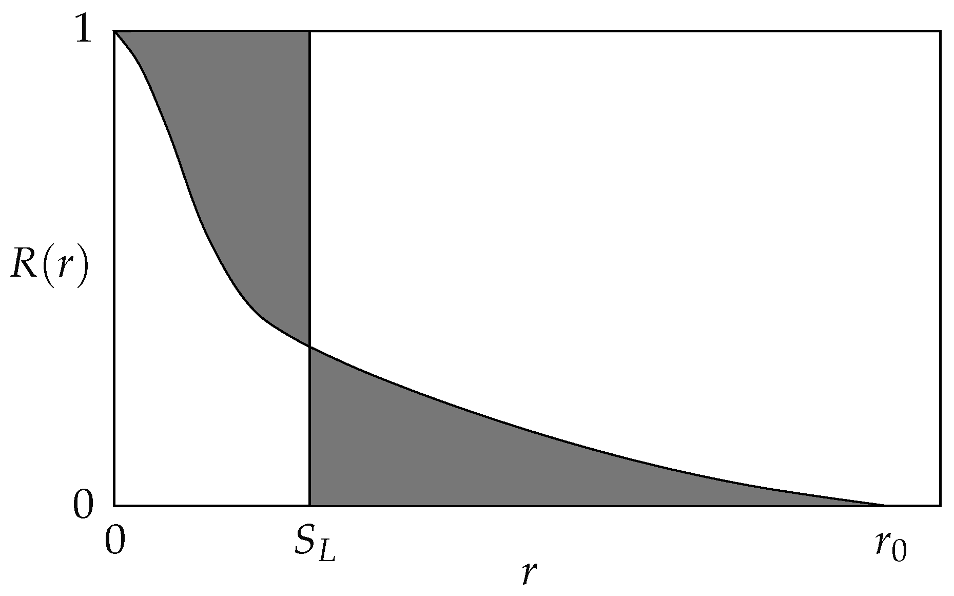
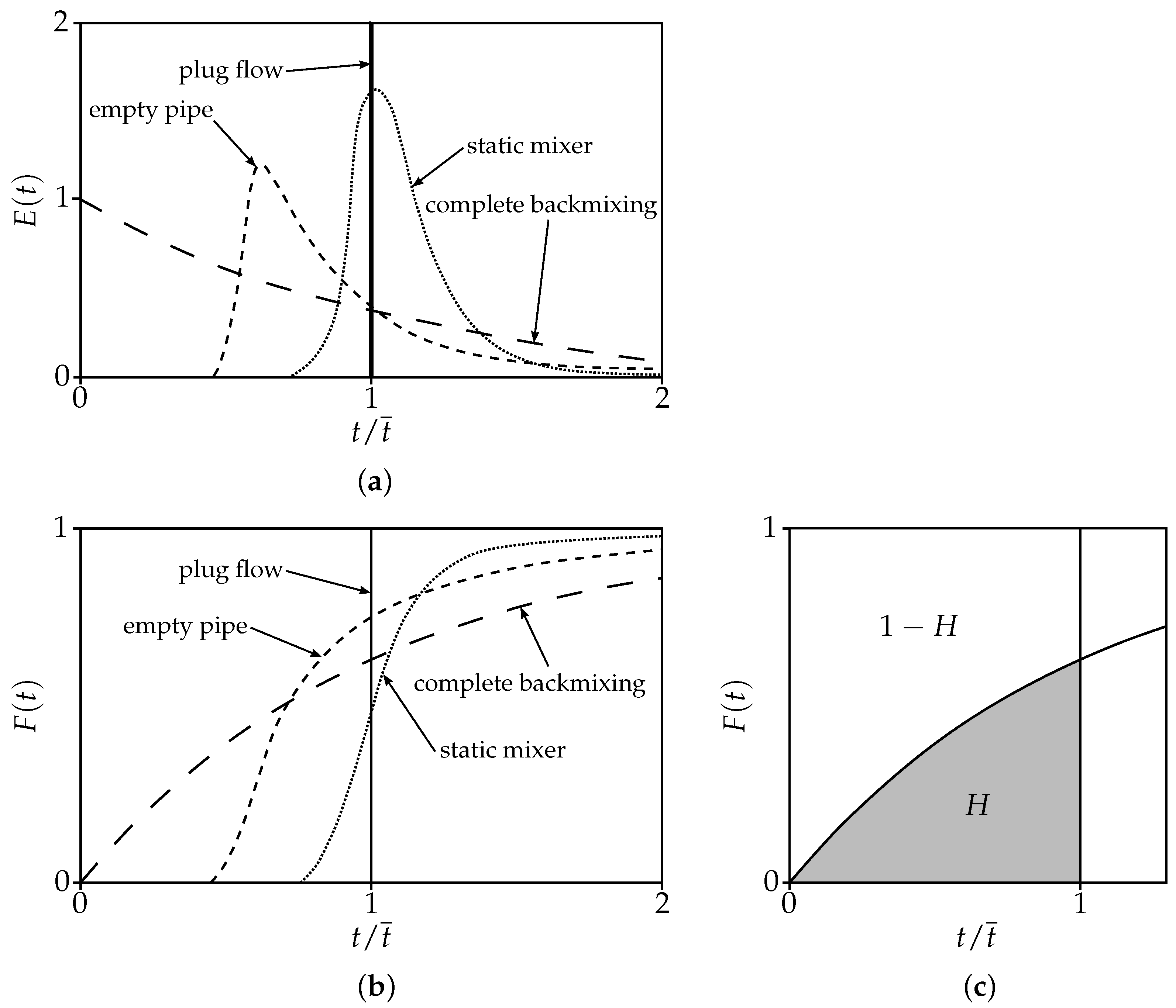
Figure 4 shows the residence time distributions
and cumulative residence time distributions
for plug flow, complete backmixing, as well as flow through an empty pipe and a static mixer.
The residence time distribution allows for determining whether the flow follows a nearly direct path from the inlet to the outlet, or whether significant portions of the fluid are separated from the main flow, causing fluid elements that entered the mixer at the same time to exit at different times [
2].
Ideally, molecules that enter the mixer simultaneously should also exit at the same time, homogeneously mixed. This ideal case is referred to as plug flow and results in a step-shaped residence time distribution at a dimensionless residence time
of 1 [
13].
In contrast, under laminar flow conditions, the parabolic velocity profile causes molecules that enter simultaneously to exit at different times, leading to a broad residence time distribution [
13].
In general, a narrower residence time distribution indicates better mixing [
2]. The broad distribution seen in complete backmixing is detrimental to reactor performance [
79,
80,
81].
Static mixers tend to narrow the residence time distribution [
23], bringing it closer to that of ideal plug flow [
12,
13,
23,
55].
The degree to which the residence time distribution approaches plug flow can be described using the first appearance time
, which is the time at which the first tracer (molecule of the mixing fluid) reaches the outlet [
13]. This is often expressed as the dimensionless first appearance time
. The value of
is 0.5 for laminar pipe flow and 1 for ideal plug flow [
13]. If the first appearance time is difficult to measure, the 5% response time, defined by
, can be used as an alternative [
13]. Another metric for quantifying the deviation from plug flow is the dimensionless variance of the residence time distribution
[
13,
59], shown in Equation (
6). It equals 0 for ideal plug flow and theoretically approaches infinity for laminar flow without diffusion [
13]. Since diffusion always occurs in real systems,
for real laminar flow assumes a finite value [
13].
As an alternative to the dimensionless variance, the coefficient of variation of residence time distribution
is also used, which is described by Equation (
7) and is likewise equal to 0 for ideal plug flow [
59]. In general, the smaller
or
, the narrower the residence time distribution and the better the mixing quality [
59].
For the integration of Equation (
6), an exponential extrapolation of the measured data is recommended [
13]. Danckwerts defined the hold-back
H, which quantifies the deviation of the residence time
t from the mean residence time
according to Equation (
8) [
51].
The hold-back
H corresponds to the area under the cumulative residence time distribution
between
and
(see
Figure 4c). For plug flow,
, and for complete backmixing,
[
51].
The residence time distribution is a measure of the temporal homogeneity of mixing [
13,
21], but it does not reflect spatial homogeneity. Therefore, it is not sufficient on its own as a measure of mixing quality [
47,
53,
54]. To describe spatial homogeneity and the mixing microstructure, other measures must be considered, such as striation thickness, interfacial area, or stretching [
13,
21,
54]. The residence time distribution can be experimentally determined by injecting a tracer pulse at the inlet and measuring the tracer concentration at a cross-section after a defined distance [
59].
2.2.3. Distributive Mixing—Describing Gradients Between Segregated Regions
Distributive mixing improves the spatial distribution of particles, droplets, or bubbles [
2,
30,
40,
55]. Key evaluation metrics include:
Standard deviation of concentration/mixing index [
30]
Intensity of segregation [
60]
Coefficient of variance (CoV) [
2,
39,
40,
55]
These metrics rely on statistical analysis of the resulting mixture, based on variance, standard deviation, probability density function, or frequency distribution (see
Figure 5). For binary mixtures (fluid A with concentration
a, and fluid B with concentration
b), metrics are symmetrical. Calculations typically use component A, ideally the minor phase (
), as
appears in denominators of several mixing indices [
82].
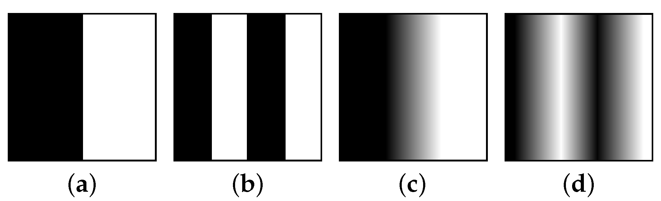
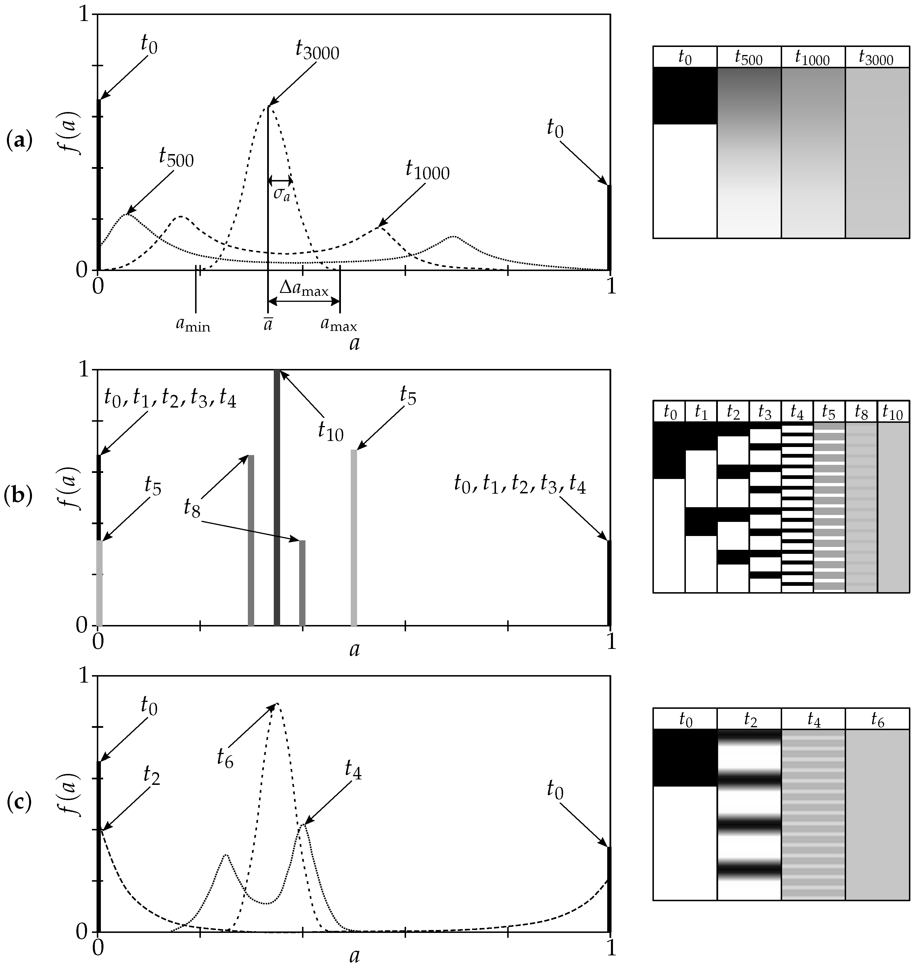
Figure 5 shows the evolution of the frequency distribution
during mixing of a 1:2 ratio of fluids A and B based on diffusion (a), mixing through baker’s transformation (b) and a combination of mixing and diffusion (c). Initially (
), two distinct peaks at
(height 1/3) and
(height 2/3) are visible. As diffusion or mixing with diffusion progresses, the peaks broaden and move toward the mean concentration
, eventually merging into a single normal distribution (see
Figure 5a,c). Further homogenization leads to a single narrow peak at
with decreasing standard deviation
, until full mixing is achieved. During mixing without diffusion, the concentration differences initially do not change, as mixing only separates and spatially distributes the regions of equal concentration. When these regions become smaller than the sample size, they are averaged, forming discrete peaks that converge to
(see
Figure 5b).
In real processes, a fully homogeneous mixture is never achieved, since small concentration variations and distinct domains remain [
33]. Mechanical rearrangement (e.g., baker’s transformation) combined with diffusion can significantly accelerate homogenization (see
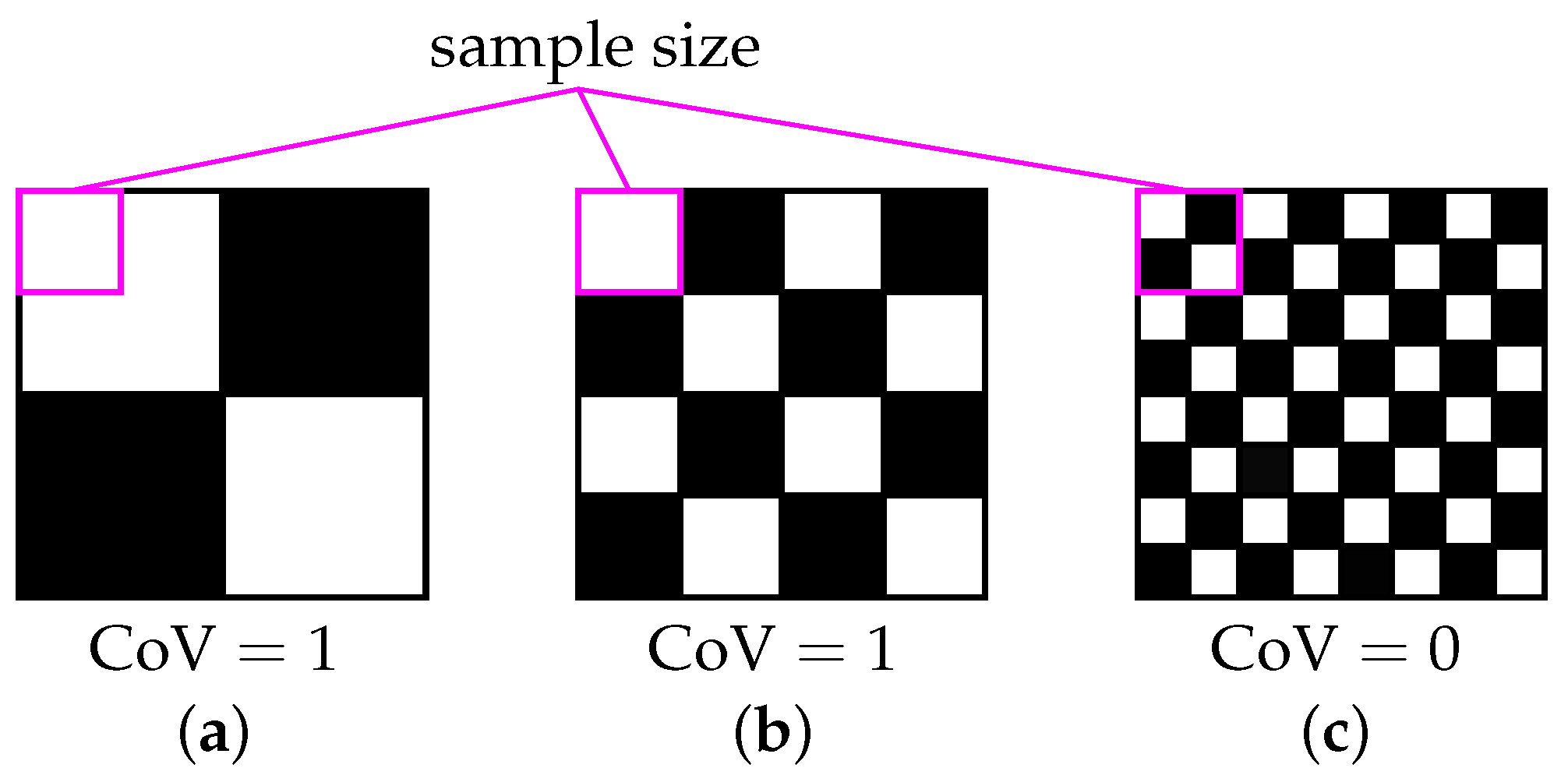
Figure 5c). In this context, Danckwerts’ scale of scrutiny refers to the smallest sample size below which segregated regions are considered mixed [
83]. It depends on the application and required level of mixing, but is often limited by the measurement technique [
71].
Danckwerts [
83] distinguishes between:
Coarse grained mixtures: The sample size includes only a few particles or molecules. Even in a perfectly random (fully mixed) system, local concentration differences appear. If a sample contains only one molecule, it can only yield values of 0 or 1 (variance = 1), falsely indicating complete segregation. Nonetheless, this is considered fully mixed since further mixing cannot improve it [
83].
Fine grained mixtures: The sample size includes many particles, so a perfectly mixed system yields uniform composition across all samples (variance ≈ 0). Incomplete mixing typically requires two parameters for characterization: the scale of segregation (domain size) and the intensity of segregation (concentration difference between domains) [
83]. A single measure is often insufficient for describing the mixture [
84].
In experiments, the smallest possible scale of scrutiny (sample size) is limited by the smallest retrievable probe, such as the pixel size of a camera or the volume of a pipette. Below this threshold, concentration differences within a probe or pixel are averaged. In CFD simulations, the minimum sample size is typically constrained by the mesh resolution, especially in multiphase flow analysis. However, in single-phase flows, the sample size can be independently defined by tracking particles through the CFD-computed flow field, irrespective of mesh size. To evaluate particle concentration distributions, samples must be chosen such that they do not overlap and contain a sufficiently large number of particles (i.e., number of samples ≪ number of particles). On average, at least 10 particles per sample are recommended to ensure statistically meaningful results [
71]. The sample size significantly influences statistical mixing metrics based on variance or standard deviation [
32,
33,
41,
71,
85,
86,
87,
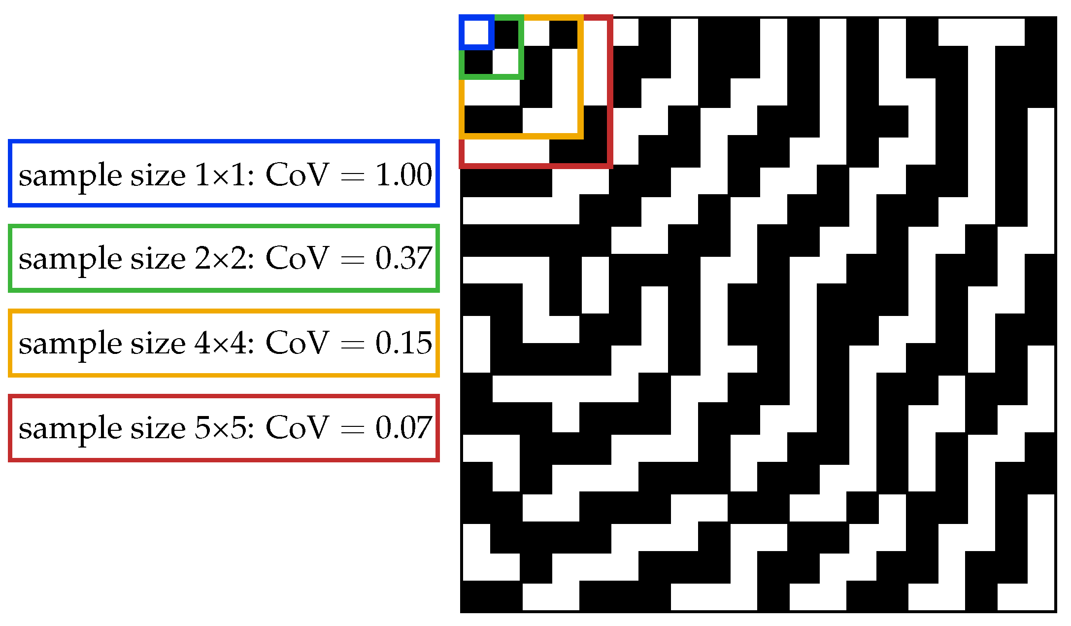
88]. Smaller sample sizes resolve local (concentration) differences more accurately, which typically results in lower calculated mixing quality [
71,
89] (see
Figure 6).
Since statistical mixing indices are affected by sample size, it is essential to report the resolution used. Reported resolutions vary considerably, which limits comparisons between studies unless it is confirmed that the mixing index value is independent of resolution. In some cases, the index stabilizes beyond a certain resolution [
90]. Examples of used resolutions include 10 × 10 [
30], 16 × 16 [
90], 64 × 64 [
65,
91], 70 × 70 [
54], 200 × 200 [
86], and 640 × 480 [
89].
In some experiments, only 4 [
92] or 9 [
38] samples are taken, which do not cover the entire cross-section; thus, both their number and spatial placement affect the mixing quality measures [
71]. At least one sample should represent the least-mixed region to provide a representative measure, which requires prior process knowledge [
71].
- (a)
Variance and Standard Deviation
Many mixing quality measures are based on the variance
or the standard deviation
of the probability density function
of concentration
a, as illustrated in
Figure 5 [
33]. The variance is calculated using Equation (
9) [
31,
33].
If the mean concentration
is unknown and estimated from local sample concentrations
or from flow rates
and
according to Equation (
10) [
13,
32], the estimated variance
is calculated using Equation (
11) [
32].
Assuming a completely segregated state (maximum variance), the concentration
only takes values 0 or 1. For a mean concentration
, the fraction of fluid A with
is
, and for fluid B with
it is
. The variance of a fully segregated system
, often assumed as the inlet condition, is calculated with Equation (
12).
For a fully homogeneous mixture, the variance approaches zero [
33]. However, only stochastic homogeneity
can be achieved in practice [
33]. For a binary mixture of fluids with equal density, it is given by Equation (
13) [
33]:
where
denotes the mean concentration of fluid A,
is the molecular volume and
the sample volume (analogous to Danckwerts’ scale of scrutiny). For a fully segregated system, the initial standard deviation
is given by Equation (
14).
Stochastic homogeneity for a binary mixture with equal density yields Equation (
15):
The mixing quality measures based on variance, standard deviation, or distribution density functions can be experimentally quantified via several concentration measurement techniques, including conductivity, color-change or decolorization reactions as well as heat release from reactions [
33,
82]. Among these methods are positron emission particle tracking (PEPT) [
93], magnetic resonance imaging (MRI) [
93,
94], (planar) laser-induced fluorescence (PLIF/LIF) [
95,
96,
97,
98], particle image velocimetry (PIV) [
96], cross-sectional sampling [
99], and conductivity measurements such as electrical resistance tomography (ERT) [
100].
For pressure-driven mixers, such as static mixers, the mixing quality measure should be flux-weighted since the mixing in cross sectional areas with high axial velocity and thus high local volumetric flow rate is more relevant than mixing close to the walls with low axial velocity [
101]. One methodology for achieving this is to select the size of the sample areas in such a way that the product of the local areas and the local axial velocities is equal [
13]. Alternatively, for areas of equal size, the concentrations of the samples can be weighted with axial velocities or volumetric flow rates [
13,
86,
93]. To calculate the flux-weighted variance
the local concentrations
are weighted by the local volumetric flow rates of the areas
relative to the volumetric flow rate of the mixer
[
86,
93], as shown in Equation (
16).
In a similar way, the volume flux-weighted standard deviation
can be obtained. The flux-weighted quantities can then be used to determine mixing quality measures. The advantage of this method is that it takes into account the residence time distribution [
101].
- (b)
Intensity of Segregation
Danckwerts defines the intensity of segregation
I for a binary mixture of fluids A and B in terms of the mean concentration
and the local concentrations
of fluid A according to Equation (
17) [
31]:
corresponds to complete segregation, while
indicates perfect homogeneity.
I quantifies the deviation of local concentrations from the mean, but provides no information on the spatial distribution or the microstructure of the mixture. For example,
I remains constant even if the size and shape of segregated regions change due to stretching, shifting, or splitting-processes that visually improve the mixture. In such cases, improvements can only be captured by dispersive mixing criteria such as the scale of segregation [
34,
35].
- (c)
Coefficient of Variation and Relative Standard Deviation
Statistical measures such as the coefficient of variation (CoV) and the relative standard deviation (RSD) are widely used for quantitative assessment of mixing quality in many industrial applications. In this context, the coefficient of variation (CoV) is calculated from the standard deviation
and the mean concentration
with Equation (
18) [
34,
39]:
When
is estimated from the measured concentrations
as
, and
is used accordingly, cf. Equations (
10) and (
11), the CoV is calculated with Equation (
19) [
13,
40]:
In industrial applications, a mixture is typically considered sufficiently homogeneous if
[
36,
37,
40]. In more sensitive cases, such as color mixing, even lower values may be required, e.g.,
[
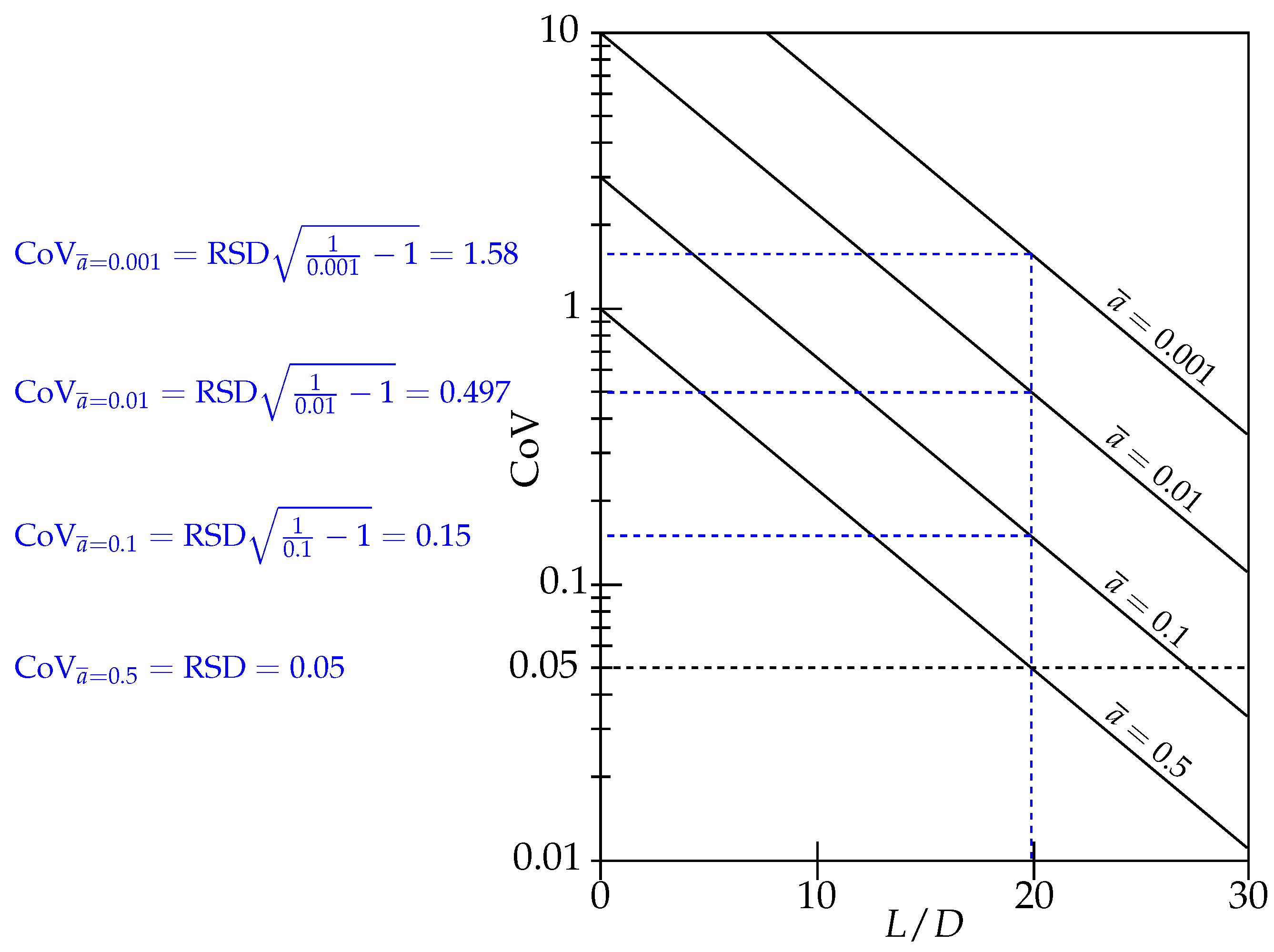
13]. The CoV depends on the composition ratio of fluids A and B. At constant mixing intensity, CoV increases with increasing imbalance between fluid fractions (i.e.,
with
), indicating reduced mixing efficiency (see
Figure 7).
To account for varying initial concentrations
, CoV can be normalized by its inlet value
, yielding the relative standard deviation (RSD) shown in Equation (
20) [
13,
34]:
CoV, RSD, and the intensity of segregation
I are interrelated according to Equation (
21):
For a given RSD and arbitrary
, the CoV can be obtained via Equation (
22):
At equal volume fractions (), it follows that .
- (d)
Absolute Deviation Measures for Qualitative Assessment
In addition to variance- and standard deviation-based approaches for evaluating mixing quality, such as the CoV, RSD or the intensity of segregation, absolute deviation measures can also be used to characterize the homogeneity of a mixture. These measures are particularly useful when technical or regulatory requirements impose limits on the maximum allowable concentration deviation [
23]. They allow for a direct assessment of how much individual local concentrations deviate from the mean value, an aspect that can be critical in reactive mixtures, pharmaceutical formulations, or color systems. Furthermore, they are intuitive and can be directly compared to defined limit values.
The maximum absolute relative concentration deviation
[
82] is calculated with Equation (
23) based on the difference between the smallest or largest concentration value,
or
, depending on which deviates more from the mean concentration
. For a symmetric distribution function, this deviation is defined as
[
82]; see
Figure 5a. This measure is often applied when a maximum deviation from the target concentration must not be exceeded [
23].
The mean absolute relative deviation
is obtained by integrating (or summing) all deviations
between the concentration frequency distribution
and the mean concentration
[
82] as shown in Equation (
24).
The degree of deviation
, introduced by Käppel [
33] and given in Equation (
25), relates the mean absolute concentration deviation
to its value before mixing,
[
33,
82].
The degree of deviation can be measured directly in decolorization experiments under the assumption of chemical equivalence between a dye and a decolorizing agent [
33]. Käppel developed a universally applicable decolorization experiment method that combines low experimental effort with high measurement accuracy [
33]. This method determines
independently of sample size, does not interfere with the flow, enables continuous measurements during the mixing process, and evaluates the entire mixed material when using multiple sensors or a movable measurement device. Furthermore, the test fluid can be reused [
33].
- (e)
Mixing Index
An alternative way to express the described measures for distributive mixing is via the mixing index
M. This index equals 0 (0%) for a completely unmixed system and 1 (100%) for a fully homogeneous mixture [
82,
102,
103,
104]. The mixing index is defined relative to various mixing quality measures, such as RSD,
,
I, CoV, or the quantities
,
, and
; see Equations (
26) to (
31). Therefore, the reference measure must be explicitly stated to ensure comparability between different publications [
82]. When the mixing index is defined in terms of
,
, or CoV,
M approaches 1 as mixing improves. However, unlike definitions based on
,
I, and
,
M does not necessarily equal 0 for a completely unmixed state at arbitrary values of the mean concentration
[
82].
There are further metrics for assessing concentration homogeneity. These are also primarily based on quantities such as
,
,
,
,
,
,
, and
, but they relate these variables in ways that differ from the measures presented here. Some of these additional indices are listed in [
33,
87].
- (f)
Describing Size of Segregated Regions Using Distributive Mixing Measures
If a sample size is defined and the concentration values within this sample are averaged, distributive mixing quality measures based on variance or standard deviation can be applied accordingly. This discretization through sampling can be purposefully employed to describe a mixture solely using statistical mixing indices [
86]. In order for the variance to decrease from 1 (complete segregation) to 0 (perfect homogeneity), two conditions must be met. First, regions of differing concentration (e.g., layers) must be smaller than the sample size. Second, the average concentration within each sample must be identical across all samples. This implies that the volume fractions of fluid A and B must be uniformly distributed across the mixer volume or cross-section and present in equal proportions in each sample. This concept is exemplified by
Figure 5b and
Figure 8.
As long as regions of differing concentration are larger than the sample size, the variance remains approximately 1, regardless of their spatial distribution in the mixer (coarse grained mixture). Therefore, a decreasing variance indicates that the regions of differing concentration are both smaller than the sample size and uniformly distributed throughout the mixer. However, the shape or distribution of these regions within each sample cannot be determined and would require other mixing indices that account for domain size or geometry. Still, in many industrial applications, knowing whether regions are smaller than a defined sample size and homogeneously distributed is sufficient for evaluating mixing quality. Consequently, many authors use mixing quality measures based on variance or standard deviation, which describe the differences in concentration between domains, as their primary or sole metric [
36,
38,
86,
89,
92,
102,
105,
106,
107,
108,
109,
110,
111,
112,
113,
114,
115].
2.2.4. Dispersive Mixing—Describing Size and Structure of Segregated Regions
Dispersive mixing describes the process of reducing the size of particle or droplet agglomerates or gas bubbles [
2,
30,
40,
55]. Dispersive mixing metrics are especially relevant in laminar flow with low diffusion, where a clear separation between regions of different concentrations exists. In some cases, these measures are only quantifiable under such conditions.
The following metrics are used to characterize dispersive mixing.
- (a)
Striation Law, Number of Striations and Interfacial Stretch
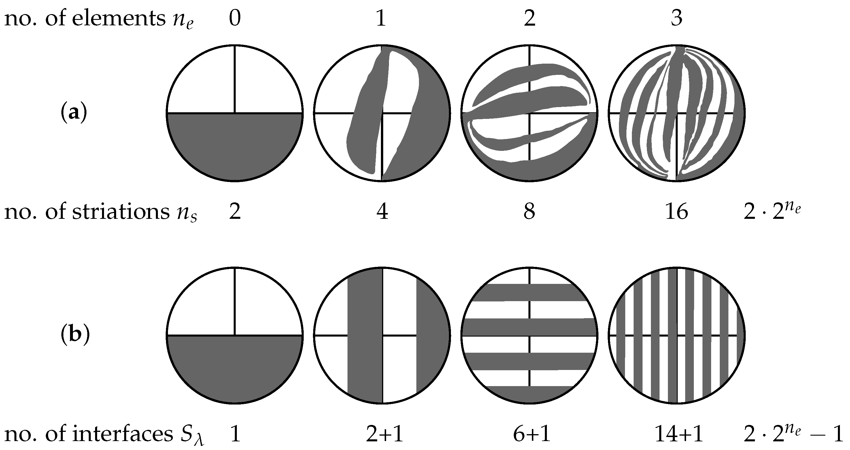
Striation laws theoretically estimate the number of striations
formed after
mixing elements, each with
flow channels, under laminar conditions. Assuming
k input components, a simple exponential relation can be derived [
23,
116] as shown in Equation (
32):
Although useful for understanding mixing progression, this law is only an approximation and may deviate from experimental results, depending on the mixer geometry [
23,
117]. The striation law (
32) neglects the significant influence of the volume flow ratio and is based on the simplified assumption that all layers have the same thickness, which does not apply under real operating conditions [
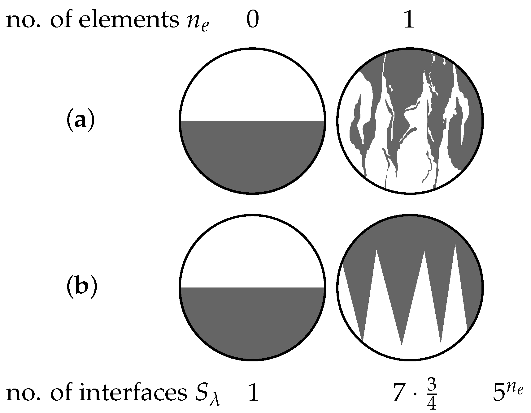
117]. Meijer et al. [
101] propose an analogue concept of the so-called interfacial stretch
, which is defined as the number of distinct interfaces formed relative to the initial configuration.
- (b)
Scale of Segregation
The scale of segregation, introduced by Danckwerts [
31], is based on the correlation coefficient
, also known as the autocorrelation function given by Equation (
33) [
31,
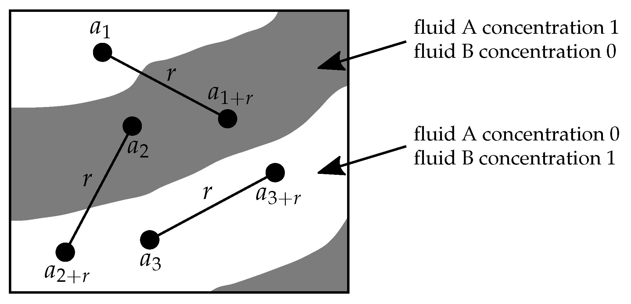
35]. It measures the statistical dependence between a concentration value
at position
i and another
at a distance
r (see
Figure 9). The average product of their deviations from the mean
is normalized by the concentration variance
:
ranges from 1 to
, indicating strong positive correlation, no correlation, or inverse correlation, respectively. Negative values may arise from periodic structures in the mixture [
31,
35]. The graph of
versus
r is called a correlogram (see
Figure 10). The distance at which
first crosses zero, denoted
, defines the correlation length [
35,
41], i.e., the scale below which domains can be considered statistically homogeneous.
Danckwerts defined the linear scale
as the integral of
according to Equation (
34) [
31]:
and the volume scale
given by Equation (
35) [
31]:
In practice,
is often computed at discrete distances. For approximating
or
, numerical integration (e.g., trapezoidal rule or curve fitting) is used. If
slowly decays to zero, identifying
directly or via a threshold (e.g.,
for 95% confidence) is often more reliable [
35,
41]. Using the striation law (
32), the theoretical scale of segregation
can be estimated in relation to the scale of segregation at the mixer inlet
according to Equation (
36) [
118].
- (c)
Interfacial Area
The interfacial area provides a quantitative measure of the surface formed between two fluids during laminar mixing, especially relevant in highly viscous systems where turbulence and diffusion are negligible. The concept of interfacial area was introduced by Spencer & Wiley [
43]. It quantifies the surface area
S formed between two fluids as a function of the initial interface
, shear, and the alignment between the interface and shear direction. Under simple (unidirectional) shear and a flat interface, the interfacial area can be calculated using Equation (
37) [
42,
43] (for simple shear
):
For curved interfaces and multidirectional shear, local shear and orientation relative to the interface must be considered. The average radius of curvature must significantly exceed half the resolution limit for meaningful quantification [
43]. Although the interfacial area reflects the dispersion of concentration regions, it does not provide information about their spatial distribution [
43].
- (d)
Striation Thickness and Striation Thinning
The concept of striation thickness was derived by Mohr et al. [
42] from the interfacial area Equation (
37). It is therefore also based solely on shear and is suitable for evaluating laminar mixing processes of highly viscous fluids. The striation thickness depends on the interfacial area according to Equation (
38), with a factor of 2 because all striations, except the two adjacent to the walls, have two interfaces [
42]. The striation thickness
is defined according to Equation (
38):
with the total interfacial area
S and the total volume of the system
V. Alternatively, the striation thickness can be defined as the ratio of the area
to the perimeter
of regions with equal fluid composition or concentration in a cross-sectional plane, e.g., at the inlet or outlet according to Equation (
39) [
46,
47,
48]:
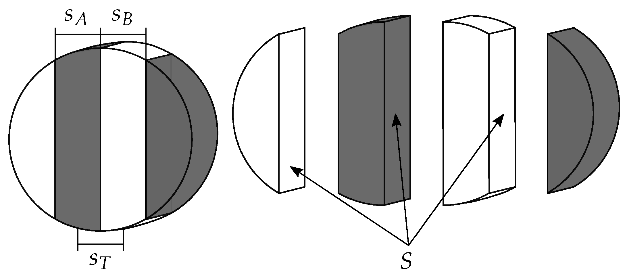
For an ideal laminar structure with constant layer thicknesses, the striation thickness can also be approximated by the average of the layer thicknesses
of fluid A and
of fluid B, as shown in Equation (
40) (see
Figure 11) [
44]:
In the case of simple (unidirectional) shear and a flat interface, the striation thickness can also be calculated using the following Equation (
41) [
42]:
with initial striation thickness (side length of cubes of the minor component)
, shear strain on the major component (product of shear rate imposed on major component and residence time)
, volume of the minor component
, viscosity of the major component
and viscosity of the minor component
. If
, the viscosity ratio is set to 1, since the minor component cannot deform faster than the major component matrix [
42].
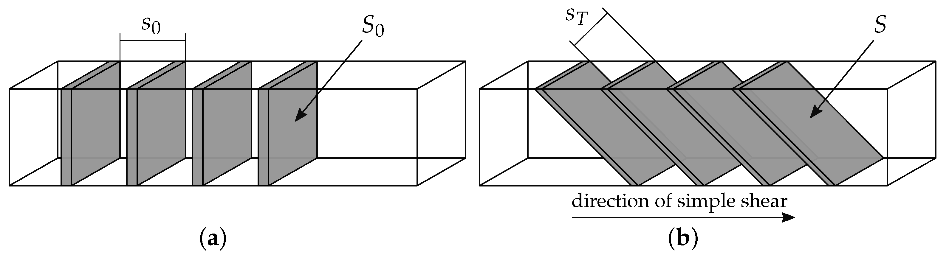
Under simple shear perpendicular to the initial striations, the striation thickness decreases and the interfacial area increases (see
Figure 12). However, the reduction in striation thickness diminishes over time, as the striations align with the direction of shear. A more efficient thinning is achieved if the shear direction changes periodically so that it remains perpendicular to the striations [
13].
The probability density function of the different striation thicknesses in the spatial structure of the partially mixed fluids is referred to as the striation thickness distribution [
45]. Employing the striation law (
32), the theoretical striation thickness
can be estimated in terms of the striation thickness at the mixer inlet
by means of Equation (
42) [
22,
117].
The striation thinning
describes the temporal change in striation thickness (e.g., between the inlet and outlet of the mixer) [
46,
48]. It is calculated with Equation (
43) and analogous to the stretching function
defined by Ottino in Equation (
48) [
50].
Integration for a constant value of
leads to Equation (
44), as derived by Fourcade et al. [
46,
48,
49].
The striation thickness can be investigated experimentally using LIF (Laser-Induced Fluorescence) systems [
119]. It can also be determined from CFD simulations using particle tracking methods, in which particles are introduced at the inlet within a small circular area (corresponding to
), and their distribution at the outlet or across various cross-sections along the mixer is evaluated (
) [
48]. However, determining striation thickness experimentally is challenging, and CFD calculations can be affected by numerical diffusion and sampling issues [
13].
- (e)
Stretching
The determination of striation thickness (and interfacial area) is often complex, as it requires resolving the actual spatial structures that form during the mixing process [
45]. A more straightforward approach is to determine the stretching of a number of points distributed throughout the entire flow field, which is closely related to both the striation thickness and interfacial area [
45]. The increase in interfacial area
S per unit volume
V is proportional, and the striation thickness
is inversely proportional to the stretching (also referred to as stretch ratio or accumulated stretching)
[
46,
54] as shown in Equation (
45):
In general, higher stretching rates indicate better mixing or micromixing quality [
65,
66]. Therefore, the stretching rate is widely used as an indicator for estimating micromixing quality [
66]. To determine the stretching rates
, the change in length
of small vectors attached to fluid particles moving with the flow (e.g., 100 vectors per particle uniformly distributed in direction [
45]) is compared to their initial length
[
54]. The stretching is then calculated according to Equation (
46) [
1,
30,
44,
54,
60,
61].
The stretching rate
can be directly computed from the deformation tensor
and the initial material orientation
using Equation (
47) [
1,
63]:
Here, is the deformation tensor , with , and denotes the initial material orientation.
The instantaneous stretching rate, or stretching function, as introduced by Ottino [
50], is defined in Equation (
48) [
1,
50]:
Here, denotes the material derivative, is the instantaneous orientation, and is the rate-of-deformation tensor.
If the time-averaged stretching function is constant and positive, the flow efficiently mixes material elements regardless of their initial position or orientation [
1,
62]. However, since both the instantaneous and averaged values depend on the time scale, the stretching function is not suited for comparing different flow fields [
1]. Instead, the (frame-invariant [
39]) stretching efficiency
provides a more appropriate metric [
1,
39,
50,
63]. It is calculated using Equation (
49).
The closer
is to 1, the more effective the flow is at generating stretching [
1].
As a symmetric tensor,
has three orthogonal eigenvectors
,
, and
associated with eigenvalues
[
1,
39,
67]. Maximum and minimum specific stretching rates occur in the directions of
and
, respectively. The corresponding maximum stretching efficiency is given by Equation (
50) [
1,
39,
67]:
For axisymmetric extensional flows,
; for squeezing flows,
; and for two-dimensional flows such as simple shear,
[
1,
39,
50,
67].
Please note that among the various dispersive mixing measures, stretching plays a central role. It is fundamentally a deformation-based quantity, derived from the local deformation tensor of infinitesimal fluid elements. At the same time, stretching provides direct insight into the chaotic nature of the flow, as quantified by the Lyapunov exponent, and serves as a basis for other scale-dependent measures, such as striation thickness and interfacial area. Consequently, while classified as deformation-based in the Introduction, stretching simultaneously captures aspects of flow chaos and scale-related phenomena, highlighting its multifunctional significance in characterizing dispersive mixing in static mixers.
- (f)
Lyapunov Exponent
In the early 1990s, laminar mixing was analyzed using tools from chaos theory [
50,
62,
64]. The Lyapunov exponent
characterizes the degree of chaos and serves as an indicator of mixing efficiency. It relates to the stretching rate
and is conceptually defined as stretching per unit time and is calculated with Equation (
51) [
46,
60]:
In steady flows through static mixers with
elements, the Lyapunov exponent can be approximated by Equation (
52), where
is the residence time per element [
61].
To ensure independence from the initial segment length,
is evaluated for infinitesimal vectors
[
61]. The Lyapunov exponent thus represents the long-term average of the instantaneous stretching rate Equation (
48) [
50], and the stretching efficiency Equation (
49) can be interpreted as a normalized Lyapunov exponent.
A positive Lyapunov exponent implies exponential growth in
, which corresponds to exponential increase in interfacial area
S and thinning of striations
[
46]; see Equations (
38) and (
45). Higher values of
indicate more chaotic systems and, in principle, improved mixing quality [
60].
To determine
and
, tracer particles with attached stretch vectors are tracked through the mixer. Their positions and vector lengths are recorded after each element to calculate
and
[
46]. For global mixing evaluation, the spatial distribution or probability density function of Lyapunov exponents from multiple initial positions can be analyzed [
63]. Note that both the stretching rate and the Lyapunov exponent represent upper bounds for the striation thinning rate
, as
is typically evaluated neglecting stretching in the primary flow direction [
46].
- (g)
Extensional Efficiency
The extensional efficiency, introduced by Manas-Zloczower [
69], is a key parameter in evaluating dispersive mixing [
2]. However, it should be considered alongside the magnitude of shear stresses in the flow field [
69].
Extensional efficiency
is defined in Equation (
53) based on the rate-of-deformation tensor
and the vorticity (spin) tensor
[
13,
30,
40,
55,
61,
68]:
Characteristic values of the extensional efficiency are:
for pure extension,
for simple shear,
Extensional flows (converging and diverging particle motion) have been shown to be more effective for dispersive mixing than simple shear flows (sliding motion) [
60,
69]. Hence, higher
values suggest better dispersion performance [
40,
68].
In static mixers,
typically ranges between 0.5 and 1, though it may vary significantly along the flow path [
13,
30]. Note that
is not frame-invariant and thus not objective in the rheological sense [
60,
61]. However, it remains suitable for comparing static mixers when the analysis is based on the same Eulerian reference frame [
60]. Moreover,
is not a direct measure of overall mixing quality, as it does not account for particle segregation [
60,
61,
68]. Nonetheless, it provides a meaningful metric for characterizing macro-mixing behavior [
66].
- (h)
Shear Rate
In laminar flows, extensional efficiency and stretching are independent of the flow rate. However, the dispersive capacity of a mixer is depending on the flow rate [
30]. Consequently, extensional efficiency and stretching are not sufficient as quality measures in this case. Flow rate-dependent quantities such as the shear rate
or mean shear rate
can be used as indicators of a mixer’s dispersion capacity, i.e., the capacity to break up droplets and bubbles [
61]. The shear rate
is derived from the rate-of-deformation tensor
using Equation (
54) [
39].
The shear rate is dependent on the pressure drop, and thus provides information about the degree of shear. To understand the relationship between energy loss and input conditions, a more appropriate interpretation should be made based on the conversion of the pressure drop to shear [
61].