
Growth of a Single Bubble Due to Super-Saturation: Comparison of Correlation-Based Modelling with CFD Simulation

 , , , and
Abstract
1. Introduction
2. Materials and Methods: Modelling of Bubble Growth
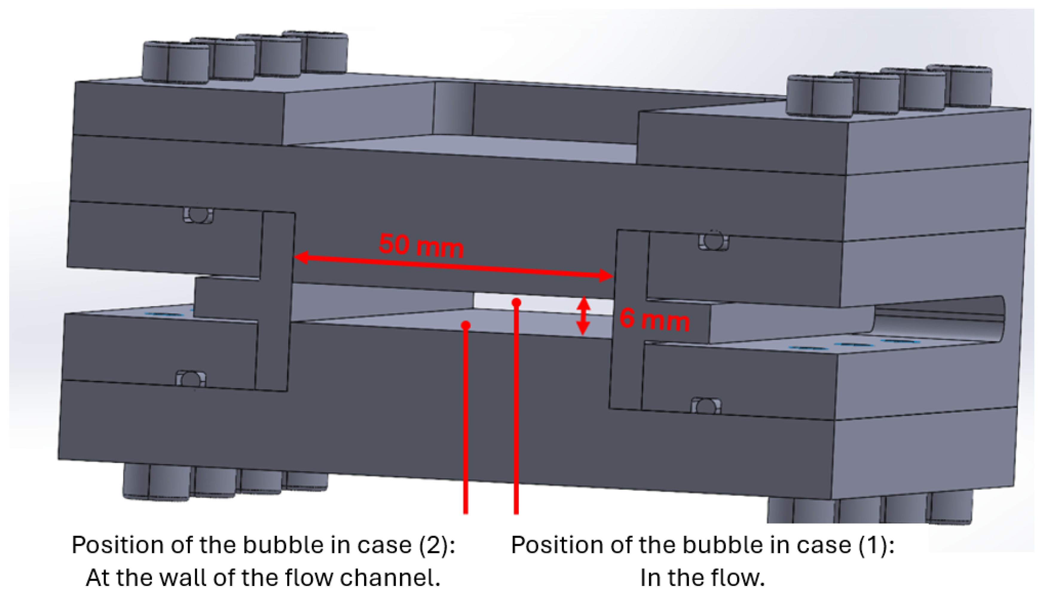
2.1. Problem Description and Boundary Conditions
2.2. CFD-Based Modelling of Bubble Growth
- Governing equations
- Model verification
2.3. Correlation-Based Modelling of Bubble Growth
2.3.1. Bubble Growth in a Flow
- (1)
- The pressure inside the bubble is calculated by applying the Laplace equation [7]. Afterwards, the density of the gas inside the bubble, , is derived.
- (2)
- Calculation of the bubble surface area, , and the bubble volume, .
- (3)
- Determination of the mass, , of the bubble.
- (4)
- The mass flow, , of dissolved oxygen molecules from the liquid bulk to the bubble can be described using a classical transport approach.
- (5)
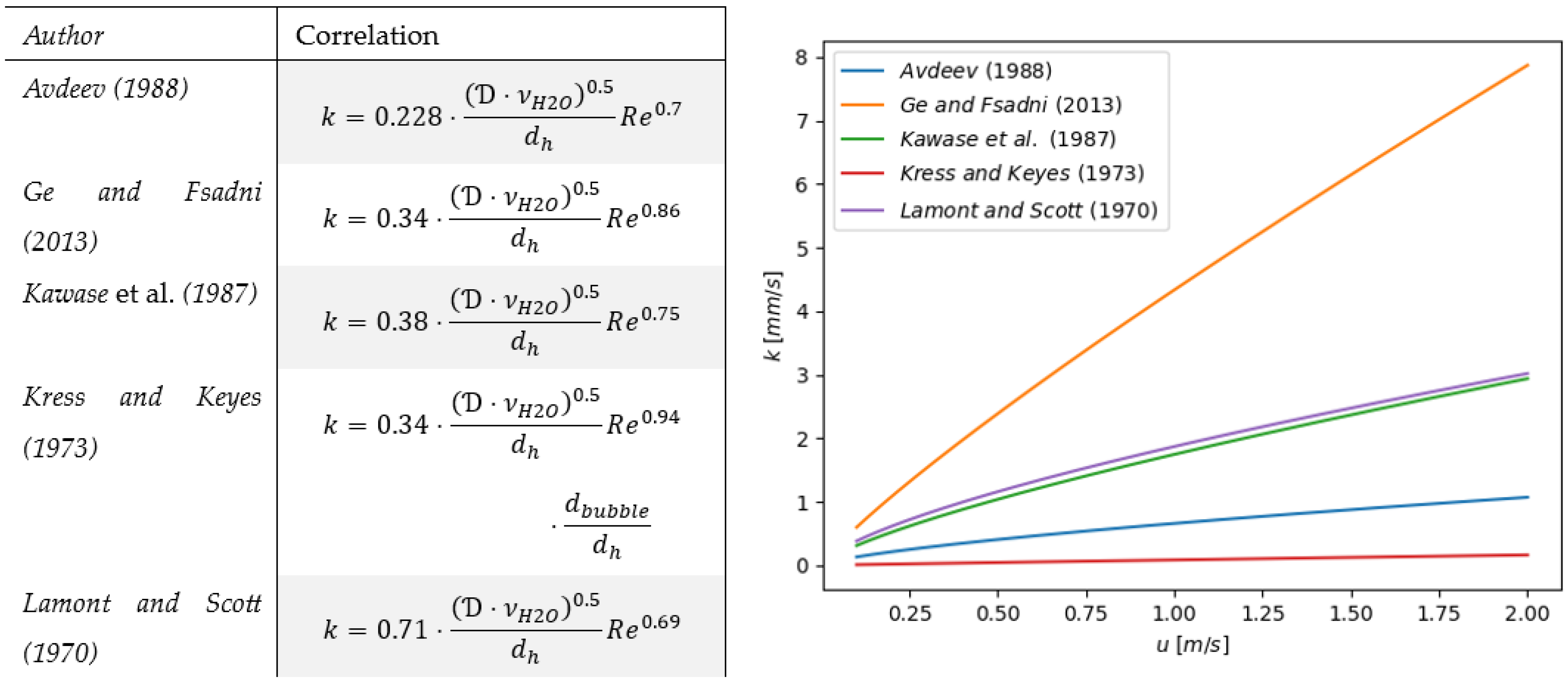
- The mass transfer coefficient, , in Equation (13) is calculated using the penetration theory. In a previous publication [17,32], it was summarized that the small eddy approach is best suited for calculating the required exposure time for bubble growth in the flow. For this reason, various correlations based on the small eddy approach for the exposure time of the penetration theory are summarized in Figure 4. In each case, the authors adjusted the coefficients of the fundamental equation in such a way that the equation most closely aligned with their experimental data.
- (6)
- The mass flow, , of dissolved gas molecules through the bubble surface leads to an increase of the mass of the gas inside the bubble. This increase results in a new mass, , after the time interval, .
- (7)
- Derivation of the radius, , of the next time step, which corresponds to a spherical bubble with the mass .
2.3.2. Bubble Growth at the Wall
3. Results and Discussion
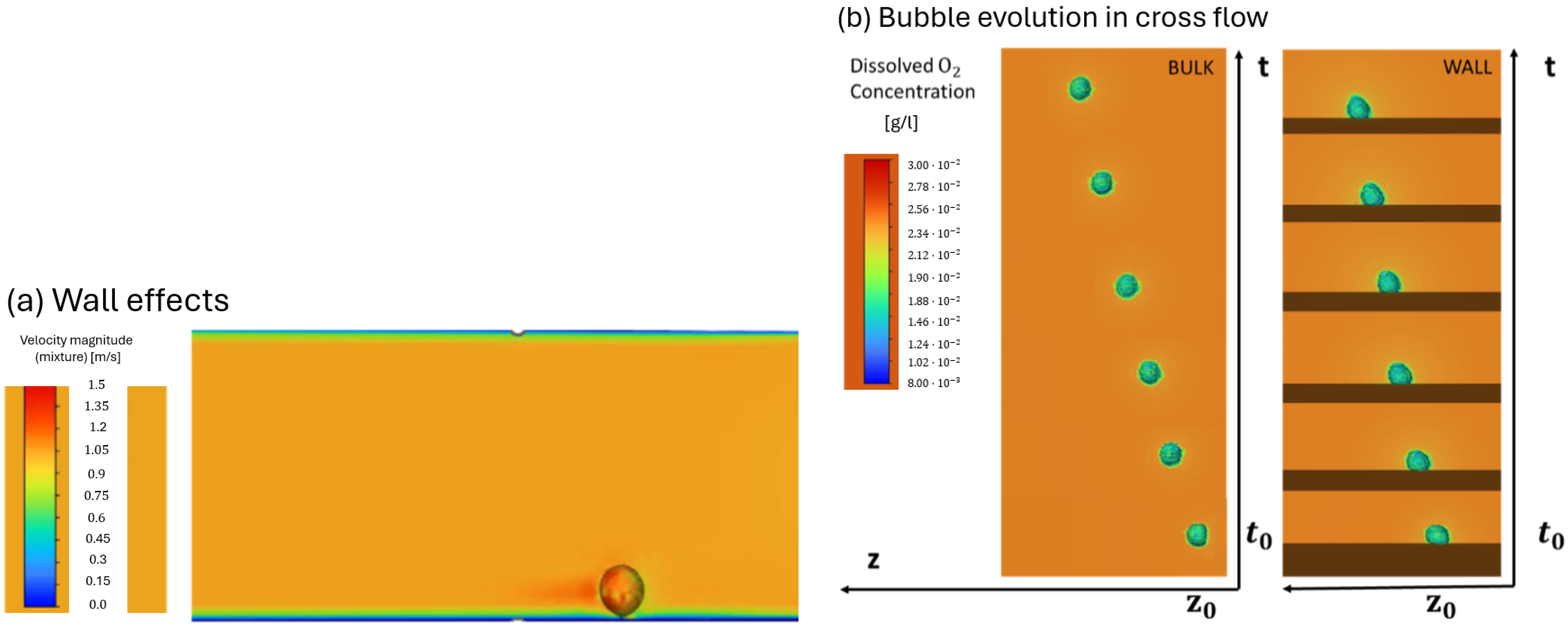
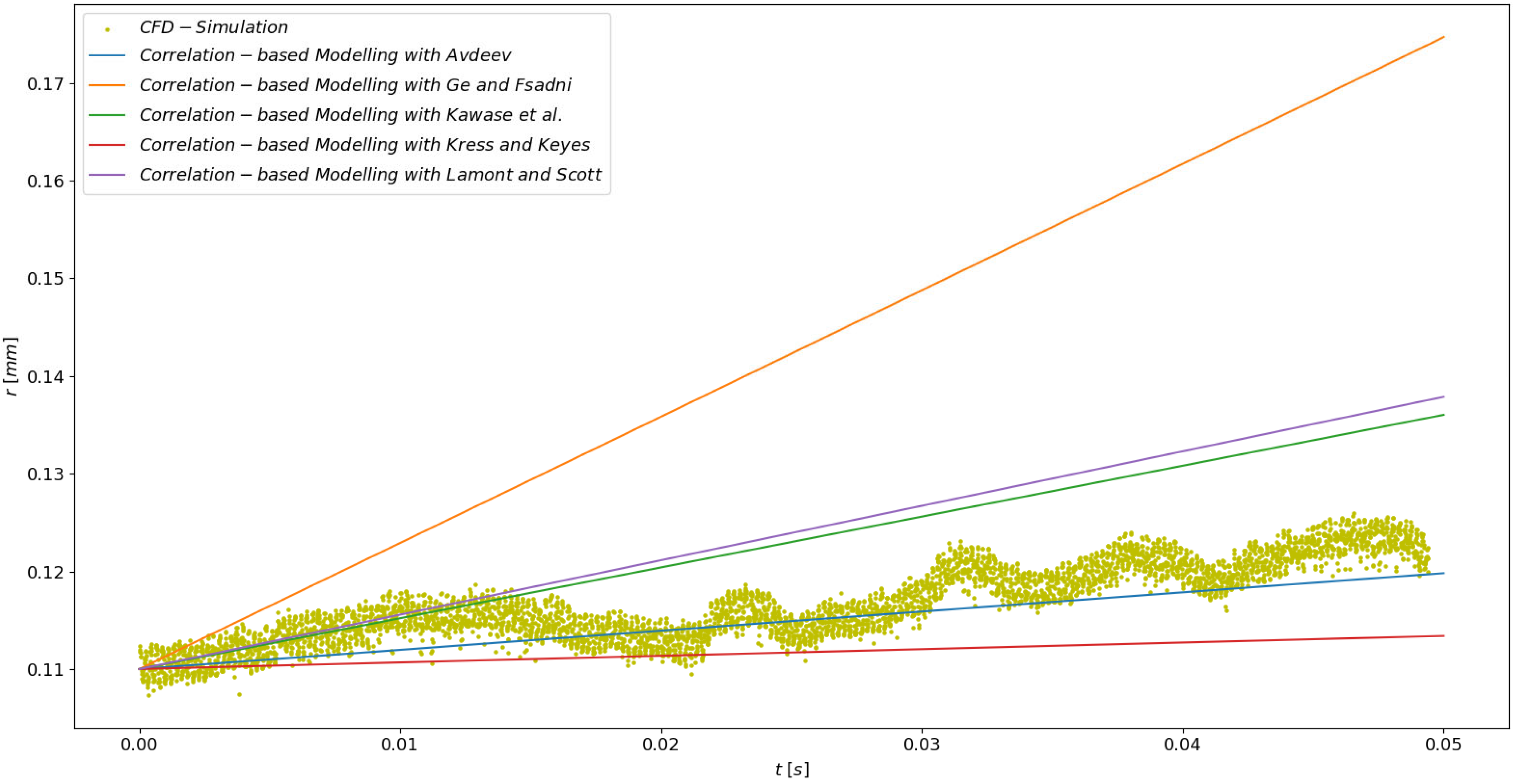
3.1. Bubble Growth in a Flow
3.2. Bubble Growth at the Wall
4. Limitations and Future Work
5. Conclusions and Outlook
Author Contributions
Funding
Data Availability Statement
Conflicts of Interest
Abbreviations
| Symbol | Description |
| bubble surface area | |
| height of channel | |
| width of channel | |
| concentration of dissolved gas | |
| Solubility | |
| diffusion coefficient | |
| hydraulic diameter | |
| minimum refined mesh sizes | |
| index of time step | |
| mass transfer coefficient | |
| mass of bubble | |
| mass flow of dissolved oxygen molecules liquid bulk to the bubble | |
| pressure | |
| bubble radius | |
| Reynolds number | |
| Time | |
| temperature | |
| flow velocity | |
| velocity profile near the wall | |
| bubble volume | |
| level of super-saturation | |
| distance from the wall | |
| surface tension | |
| static contact angle | |
| kinematic viscosity water |
References
- Barker, G.; Jefferson, B.; Judd, S. The control of bubble size in carbonated beverages. Chem. Eng. Sci. 2002, 57, 565–573. [Google Scholar] [CrossRef]
- Uzel, S.; Chappell, M.A.; Payne, S.J. Modeling the cycles of growth and detachment of bubbles in carbonated beverages. J. Phys. Chem. B 2006, 110, 7579–7586. [Google Scholar] [CrossRef] [PubMed]
- Ge, Y.T.; Fsadni, A.M.; Wang, H.S. Bubble dissolution in horizontal turbulent bubbly flow in domestic central heating system. Appl. Energy 2013, 108, 477–485. [Google Scholar] [CrossRef]
- Hurwitz, S.; Navon, O. Bubble nucleation in rhyolitic melts: Experiments at high pressure, temperature, and water content. Earth Planet. Sci. Lett. 1994, 122, 267–280. [Google Scholar] [CrossRef]
- Lavenson, D.M.; Kelkar, A.V.; Daniel, A.B.; Mohammad, S.A.; Kouba, G.; Aichele, C.P. Gas evolution rates—A critical uncertainty in challenged gas-liquid separations. J. Pet. Sci. Eng. 2016, 147, 816–828. [Google Scholar] [CrossRef]
- Jones, S.F.; Evans, G.M.; Galvin, K.P. Bubble nucleation from gas cavities—A review. Adv. Colloid Interface Sci. 1999, 80, 27–50. [Google Scholar] [CrossRef]
- Liger-Belair, G. The physics and chemistry behind the bubbling properties of champagne and sparkling wines: A state-of-the-art review. J. Agric. Food Chem. 2005, 53, 2788–2802. [Google Scholar] [CrossRef]
- Lubetkin, S.D. The fundamentals of bubble evolution. Chem. Soc. Rev. 1995, 24, 243. [Google Scholar] [CrossRef]
- Scriven, L.E. On the dynamics of phase growth. Chem. Eng. Sci. 1959, 10, 1–13. [Google Scholar] [CrossRef]
- Shafer, N.E.; Zare, R.N. Through a Beer Glass Darkly. Phys. Today 1991, 44, 48–52. [Google Scholar] [CrossRef]
- Arefmanesh, A.; Advani, S.G.; Michaelides, E.E. An accurate numerical solution for mass diffusion-induced bubble growth in viscous liquids containing limited dissolved gas. Int. J. Heat Mass Transf. 1992, 35, 1711–1722. [Google Scholar] [CrossRef]
- Jones, S.F.; Evans, G.M.; Galvin, K.P. The cycle of bubble production from a gas cavity in a supersaturated solution. Adv. Colloid Interface Sci. 1999, 80, 51–84. [Google Scholar] [CrossRef]
- Liger-Belair, G. How many bubbles in your glass of bubbly? J. Phys. Chem. B 2014, 118, 3156–3163. [Google Scholar] [CrossRef] [PubMed]
- Enríquez, O.R.; Sun, C.; Lohse, D.; Prosperetti, A.; van der Meer, D. The quasi-static growth of CO2 bubbles. J. Fluid Mech. 2014, 741, R1. [Google Scholar] [CrossRef]
- Kwak, H.-Y.; Kang, K.-M. Gaseous Bubble Nucleation Under Shear Flow. In Proceedings of the ASME 2009 7th International Conference on Nanochannels, Microchannels and Minichannels. ASMEDC 2009, Pohang, Republic of Korea, 22–24 June 2009; pp. 1063–1068. [Google Scholar]
- Groß, T.F.; Bauer, J.; Ludwig, G.; Fernandez Rivas, D.; Pelz, P.F. Bubble nucleation from micro-crevices in a shear flow. Exp. Fluids 2018, 59, 12. [Google Scholar] [CrossRef]
- Manthey, J.; Guesmi, M.; Schab, R.; Unz, S.; Beckmann, M. Bubble evolution due to super-saturation in the cooling circuit of the PEM-electrolysis. Int. J. Hydrogen Energy 2024, 78, 433–442. [Google Scholar] [CrossRef]
- Heinrich, J.; Ränke, F.; Schwarzenberger, K.; Yang, X.; Baumann, R.; Marzec, M.; Lasagni, A.F.; Eckert, K. Functionalization of Ti64 via Direct Laser Interference Patterning and Its Influence on Wettability and Oxygen Bubble Nucleation. ACS Langmuir 2024, 40, 2918–2929. [Google Scholar] [CrossRef]
- Guesmi, M.; Manthey, J.; Unz, S.; Schab, R.; Beckmann, M. Gas Liquid flow pattern prediction in horizontal and slightly inclined pipes: From mechanistic modelling to machine learning. Appl. Math. Model. 2024, 138, 115748. [Google Scholar] [CrossRef]
- Moeng, C.-H.; Sullivan, P.P. NUMERICAL MODELS|Large-Eddy Simulation. In Encyclopedia of Atmospheric Sciences; Elsevier: Amsterdam, The Netherlands, 2015; pp. 232–240. [Google Scholar]
- Cho, M.; Lozano-Durán, A.; Moin, P.; Ilhwan Park, G. Wall-Modeled Large-Eddy Simulation of Turbulent Boundary Layers with Mean-Flow Three-Dimensionality. AIAA J. 2021, 59, 1707–1717. [Google Scholar] [CrossRef]
- Zhou, D.; Bae, H.J. Sensitivity analysis of wall-modeled large-eddy simulation for separated turbulent flow. J. Comput. Phys. 2024, 506, 112948. [Google Scholar] [CrossRef]
- Hirt, C.; Nichols, B. Volume of fluid (VOF) method for the dynamics of free boundaries. J. Comput. Phys. 1981, 39, 201–225. [Google Scholar] [CrossRef]
- Yokoi, K. Anti-diffusion method for coupled level set and volume of fluid, volume of fluid, and tangent of hyperbola for interface capturing methods. Phys. Fluids 2024, 36, 092121. [Google Scholar] [CrossRef]
- Vachaparambil, K.J.; Einarsrud, K.E. Numerical simulation of continuum scale electrochemical hydrogen bubble evolution. Appl. Math. Model. 2021, 98, 343–377. [Google Scholar] [CrossRef]
- Nguyen, V.-T.; Park, W.-G. A volume-of-fluid (VOF) interface-sharpening method for two-phase incompressible flows. Comput. Fluids 2017, 152, 104–119. [Google Scholar] [CrossRef]
- Potgieter, J.; Lombaard, L.; Hannay, J.; Moghimi, M.A.; Valluri, P.; Meyer, J.P. Adaptive mesh refinement method for the reduction of computational costs while simulating slug flow. Int. Commun. Heat Mass Transf. 2021, 129, 105702. [Google Scholar] [CrossRef]
- Piomelli, U.; Moin, P.; Ferziger, J.H. Model consistency in large eddy simulation of turbulent channel flows. Phys. Fluids 1988, 31, 1884–1891. [Google Scholar] [CrossRef]
- Cox, R.G. The dynamics of the spreading of liquids on a solid surface. Part 1. Viscous flow. J. Fluid Mech. 1986, 168, 169. [Google Scholar] [CrossRef]
- Zhang, J.; Ding, W.; Hampel, U. How droplets pin on solid surfaces. J. Colloid Interface Sci. 2023, 640, 940–948. [Google Scholar] [CrossRef]
- Epstein, P.S.; Plesset, M.S. On the Stability of Gas Bubbles in Liquid-Gas Solutions. J. Chem. Phys. 1950, 18, 1505–1509. [Google Scholar] [CrossRef]
- Manthey, J.; Guesmi, M.; Schab, R.; Unz, S.; Beckmann, M. A sensitivity analysis on the bubble departure diameter for bubble growth due to oxygen super-saturation in highly purified water. Int. J. Thermofluids 2023, 18, 100327. [Google Scholar] [CrossRef]
- Avdeev, A. Growth, condensation and dissolution of vapor and gas bubbles in turbulent flows at medium Reynolds number. Teplofiz. Vysok. Temp. 1990, 28, 540–546. [Google Scholar]
- Lezhnin, S.; Eskin, D.; Leonenko, Y.; Vinogradov, O. Dissolution of air bubbles in a turbulent water pipeline flow. Heat Mass Transf. 2003, 39, 483–487. [Google Scholar] [CrossRef]
- Fsadni, A.M.; Ge, Y. Micro bubble formation and bubble dissolution in domestic wet central heating systems. EPJ Web Conf. 2012, 25, 01016. [Google Scholar] [CrossRef]
- Kawase, Y.; Halard, B.; Moo-Young, M. Theoretical prediction of volumetric mass transfer coefficients in bubble columns for Newtonian and non-Newtonian fluids. Chem. Eng. Sci. 1987, 42, 1609–1617. [Google Scholar] [CrossRef]
- Kress, T.S.; Keyes, J.J. Liquid phase controlled mass transfer to bubbles in cocurrent turbulent pipeline flow. Chem. Eng. Sci. 1973, 28, 1809–1823. [Google Scholar] [CrossRef]
- Lamont, J.C.; Scott, D.S. An eddy cell model of mass transfer into the surface of a turbulent liquid. AIChE J. 1970, 16, 513–519. [Google Scholar] [CrossRef]
- Zeng, L.Z.; Klausner, J.F.; Bernhard, D.M.; Mei, R. A unified model for the prediction of bubble detachment diameters in boiling systems—II. Flow boiling. Int. J. Heat Mass Transf. 1993, 36, 2271–2279. [Google Scholar] [CrossRef]
- VDI-Gesellschaft Verfahrenstechnik und Chemieingenieurwesen. VDI-Wärmeatlas; Springer: Berlin/Heidelberg, Germany, 2013. [Google Scholar]
- Al-Hayes, R.; Winterton, R. Bubble growth in flowing liquids. Int. J. Heat Mass Transf. 1981, 24, 213–221. [Google Scholar] [CrossRef]
- Alves, S.S.; Vasconcelos, J.M.; Orvalho, S.P. Mass transfer to clean bubbles at low turbulent energy dissipation. Chem. Eng. Sci. 2006, 61, 1334–1337. [Google Scholar] [CrossRef]
- Farsoiya, P.K.; Popinet, S.; Deike, L. Bubble-mediated transfer of dilute gas in turbulence. J. Fluid Mech. 2021, 920, A34. [Google Scholar] [CrossRef]
- Lamont, J.C.; Scott, D.S. Mass transfer from bubbles in cocurrent flow. Can. J. Chem. Eng. 1966, 44, 201–208. [Google Scholar] [CrossRef]
- Avdeev, A.A. Bubble Systems; Springer International Publishing: Cham, Switzerland, 2016. [Google Scholar]


| Surface Tension | Concentration of Dissolved Oxygen | Solubility | Kinematic Viscosity Water | Density Oxygen | Diffusion Coefficient | Reynolds Number |
|---|---|---|---|---|---|---|
| Parameter | Default Value | Description |
|---|---|---|
| Wall model type | S-omega | The wall model used for WMLES |
| LES turbulence model | Dynamic Smagorinsky | Subgrid-scale model for LES turbulence |
| Matching location (y+) | 200 | Dimensionless wall distance where wall model connects with LES region |
| Wall model turbulent viscosity | S-omega model | Based on the S-omega equation |
| Damping function | Enabled | Helps transition from RANS to LES |
| Blending function | Enabled | Smooth transition between wall model and LES |
| Turbulent Prandtl number | 0.9 | Ratio of momentum diffusivity to thermal diffusivity |
| Wall heat transfer modelling | Enabled | Uses wall function approach for heat transfer if energy equation is solved |
| Wall roughness | Smooth wall | No roughness (can be adjusted) |
| Wall model time stepping | Implicit | Temporal integration method for wall model equations |
| Time averaging for wall model | Enabled | Averages flow quantities used in wall model |
| Averaging time window | User-defined or 0.1–0.5 s | Duration for time-averaging (if enabled) |
| SST damping switch | Off | Only used for specific variants |
Disclaimer/Publisher’s Note: The statements, opinions and data contained in all publications are solely those of the individual author(s) and contributor(s) and not of MDPI and/or the editor(s). MDPI and/or the editor(s) disclaim responsibility for any injury to people or property resulting from any ideas, methods, instructions or products referred to in the content. |
© 2025 by the authors. Licensee MDPI, Basel, Switzerland. This article is an open access article distributed under the terms and conditions of the Creative Commons Attribution (CC BY) license (https://creativecommons.org/licenses/by/4.0/).
Share and Cite
Manthey, J.; Ding, W.; Mehdipour, H.; Guesmi, M.; Unz, S.; Hampel, U.; Beckmann, M. Growth of a Single Bubble Due to Super-Saturation: Comparison of Correlation-Based Modelling with CFD Simulation. ChemEngineering 2025, 9, 63. https://doi.org/10.3390/chemengineering9030063
Manthey J, Ding W, Mehdipour H, Guesmi M, Unz S, Hampel U, Beckmann M. Growth of a Single Bubble Due to Super-Saturation: Comparison of Correlation-Based Modelling with CFD Simulation. ChemEngineering. 2025; 9(3):63. https://doi.org/10.3390/chemengineering9030063
Chicago/Turabian StyleManthey, Johannes, Wei Ding, Hossein Mehdipour, Montadhar Guesmi, Simon Unz, Uwe Hampel, and Michael Beckmann. 2025. "Growth of a Single Bubble Due to Super-Saturation: Comparison of Correlation-Based Modelling with CFD Simulation" ChemEngineering 9, no. 3: 63. https://doi.org/10.3390/chemengineering9030063
APA StyleManthey, J., Ding, W., Mehdipour, H., Guesmi, M., Unz, S., Hampel, U., & Beckmann, M. (2025). Growth of a Single Bubble Due to Super-Saturation: Comparison of Correlation-Based Modelling with CFD Simulation. ChemEngineering, 9(3), 63. https://doi.org/10.3390/chemengineering9030063