Improved Fault Detection in Chemical Engineering Processes via Non-Parametric Kolmogorov–Smirnov-Based Monitoring Strategy

Abstract

Fault detection is crucial in maintaining reliability, safety, and consistent product quality in chemical engineering processes. Accurate fault detection allows for identifying anomalies, signaling deviations from the system’s nominal behavior, ensuring the system operates within desired performance parameters, and minimizing potential losses. This paper presents a novel semi-supervised data-based monitoring technique for fault detection in multivariate processes. To this end, the proposed approach merges the capabilities of Principal Component Analysis (PCA) for dimensionality reduction and feature extraction with the Kolmogorov–Smirnov (KS)-based scheme for fault detection. The KS indicator is computed between the two distributions in a moving window of fixed length, allowing it to capture sensitive details that enhance the detection of faults. Moreover, no labeling is required when using this fault detection approach, making it flexible in practice. The performance of the proposed PCA–KS strategy is assessed for different sensor faults on benchmark processes, specifically the Plug Flow Reactor (PFR) process and the benchmark Tennessee Eastman (TE) process. Different sensor faults, including bias, intermittent, and aging faults, are considered in this study to evaluate the proposed fault detection scheme. The results demonstrate that the proposed approach surpasses traditional PCA-based methods. Specifically, when applied to PFR data, it achieves a high average detection rate of 98.31% and a low false alarm rate of 0.25%. Similarly, when applied to the TE process, it provides a good average detection rate of 97.27% and a false alarm rate of 6.32%. These results underscore the efficacy of the proposed PCA–KS approach in enhancing the fault detection of high-dimensional processes.

1. Introduction

Efficient and continuous monitoring of key process variables is crucial for optimizing complex chemical and petrochemical processes [1,2]. The primary objective is not only to enhance productivity but also to prevent catastrophic incidents in the event of a failure [3,4]. Several severe accidents have underscored the importance of timely fault detection in chemical and petrochemical plants globally over the past few decades. Examples include the tragic Union Carbide accident in Bhopal, India, in 1984, where a massive toxic gas leak resulted in over 3000 deaths and severe injuries to 400,000 residents [5,6]. Another notable incident is the Piper Alpha accident in 1988 involving a North Sea oil production platform, where an explosion resulted in the deaths of 167 individuals [7]. In 2000, the Mina Al-Ahmedi accident in Kuwait, caused by a condensate line failure in a refinery plant, resulted in 5 deaths and 50 injuries [8]. Hence, fault detection in chemical engineering processes is essential for maintaining safety, product quality, and operational efficiency while preventing costly accidents and environmental harm [9].

The evolution of process automation has transformed the industry, enabling the systematic conversion of natural resources into final products without constant human oversight. The integration of smart sensor networks and distributed control systems has further complicated the dynamics of chemical industries, introducing new challenges. This complexity has given rise to frequent hazards, such as emission discharges and explosions in processing plants, posing serious threats to both human health and the environment. Manual errors, inadequate maintenance, and sensor malfunctions are among the primary causes of these faults. Timely identification and mitigation of faults are critical for ensuring regulatory compliance and cost-effective operations [10]. Over the last few decades, numerous fault detection methods have been developed and can be categorized into two primary categories: model-based and data-based approaches [11,12].

Model-based methods are based on prior knowledge of the system or process being monitored. These techniques involve constructing mathematical models that encapsulate the anticipated behavior of the system under normal operating conditions. Any deviation from these model predictions serves as an indicator of a fault or anomaly. Model-based approaches are renowned for their precision but necessitate an in-depth comprehension of the system and its dynamics, often making their development and maintenance challenging [8]. Numerous model-based methods have been developed in the literature, including observer-based [13], parity-based [14], and interval-based approaches [15]. Of course, the accuracy of these model-based monitoring methods relies on the precision of the models employed. In contrast, data-based methods for fault detection do not rely on explicit models, but instead leverage historical or real-time data for detecting anomalies or deviations from desired performance [16]. These methods are inherently data driven and excel in detecting faults in intricate systems where developing precise models is difficult [17]. Data-based techniques, including statistical methods and machine-learning algorithms, are gaining prominence due to their adaptability to shifting process conditions and ability to detect faults without prior system knowledge [18,19]. The choice between model-based and data-based fault detection methods is contingent on various factors, including the system’s characteristics, data availability, and the level of system understanding. In practical applications, a combination of these methods is often employed to enhance the reliability and accuracy of fault detection across a spectrum of industrial and engineering contexts [17].

In data-driven fault detection methods, there are univariate statistical techniques and multivariate statistical monitoring methods. Univariate methods are primarily designed to monitor individual variables independently. They are useful when monitoring the behavior of a single process variable over time [20]. Prominent examples of univariate methods include the Cumulative Sum (CUSUM) [21,22] and Exponentially Weighted Moving Average (EWMA) [23] control charts. These methods are simple and effective for identifying deviations from expected values or trends in a single variable. However, they do not consider interactions or correlations between variables, which can lead to missed detections when dealing with multivariate processes. Multivariate methods, on the other hand, are specifically designed for monitoring systems with multiple interrelated variables [24]. These methods consider the relationships and dependencies between different variables in the system. They are well-suited for detecting faults that affect multiple variables simultaneously [18]. Multivariate techniques are invaluable in industries with intricate, interdependent processes, such as chemical manufacturing and petrochemicals, where a fault in one part of the system can propagate through multiple variables, leading to significant consequences [25]. Over the past few decades, various multivariate monitoring techniques have been extensively utilized in fault detection and diagnosis. These include Principal Component Analysis (PCA), Partial Least Squares (PLS), Fisher Discriminant Analysis (FDR), and Principal Component Regression (PCR) [12].

Specifically, PCA-based monitoring strategies have been instrumental in addressing various fault detection challenges over the past two decades [26,27,28]. The PCA model selectively retains a few key Principal Components (PCs) that encapsulate systematic data variations. This model is further enhanced with two fault indicators: $T^2$ for monitoring the modeled subspace and Squared Prediction Error (SPE) or Q for monitoring the residual subspace [3]. Numerous extensions of the conventional PCA approach have emerged to accommodate the dynamic and evolving nature of industrial processes. Notably, a recursive PCA method has been developed, which leverages the PCA model to compute a recursive model, considering the time-varying nature of the industrial process [29,30]. Dynamic PCA (DPCA) has been introduced to consider process dynamics by incorporating information from lagged data in the model [31]. Additionally, the Multi-Scale PCA (MSPCA) approach combines PCA with wavelet analysis to enable multiscale de-noising, enhancing fault detection capabilities [32]. For capturing non-linearities in process data, an improved non-linear variant known as the kernel PCA strategy has been widely used [33]. Once constructed, the multivariate model plays a pivotal role in fault detection when applied to new processes, with the support of fault indicators.

However, conventional PCA-based monitoring indices such as $T^2$ and Q statistics prove relatively inefficient at detecting small changes [11]. Their decision making relies solely on the latest observation, limiting their ability to detect faults with small magnitudes [34]. Enhancing the capability to detect these faults can be achieved by employing a monitoring chart that leverages information spanning the entire process history. Over the years, various parametric and non-parametric tests have been explored to enhance the detection of incipient faults. Parametric tests assume that samples are drawn from a population following a probability distribution [35]. Within the parametric framework, several commonly applied tests include the Generalized Likelihood Ratio [36], Kullback–Leibler Divergence [37], Continuous Rank Probability Score [10], Jensen–Shannon Divergence [38], and Hellinger’s Distance [39]. However, it is important to note that these tests may fail when the underlying assumptions do not accurately represent the data. Non-parametric statistical tests, in contrast, operate without making any assumptions about the data being drawn from a specific distribution [40]. Their strength lies in their ability to adapt to a broader range of data scenarios, making them inherently more robust [41].

This work introduces an effective monitoring approach that improves fault detection in multivariate correlated data. The approach combines PCA for dimensionality reduction and the Kolmogorov–Smirnov (KS) non-parametric test. PCA extracts relevant information from the data, while the KS test contributes to fault detection with its sensitivity to deviations. The major contributions of the paper include the following:

• A novel fault detection strategy, termed PCA–KS, is developed by merging the Kolmogorov–Smirnov (KS) test with Principal Component Analysis (PCA). PCA serves a dual purpose in dimensionality reduction and residual generation. Under normal operating conditions, residuals cluster around zero, reflecting the influence of measurement noise and uncertainties. However, when faults are present, residuals deviate considerably from zero. The Kolmogorov–Smirnov test is subsequently employed to evaluate these residuals for fault detection. Notably, this semi-supervised approach does not require prior knowledge of the system, enhancing its practicality and adaptability across various industrial and engineering applications.
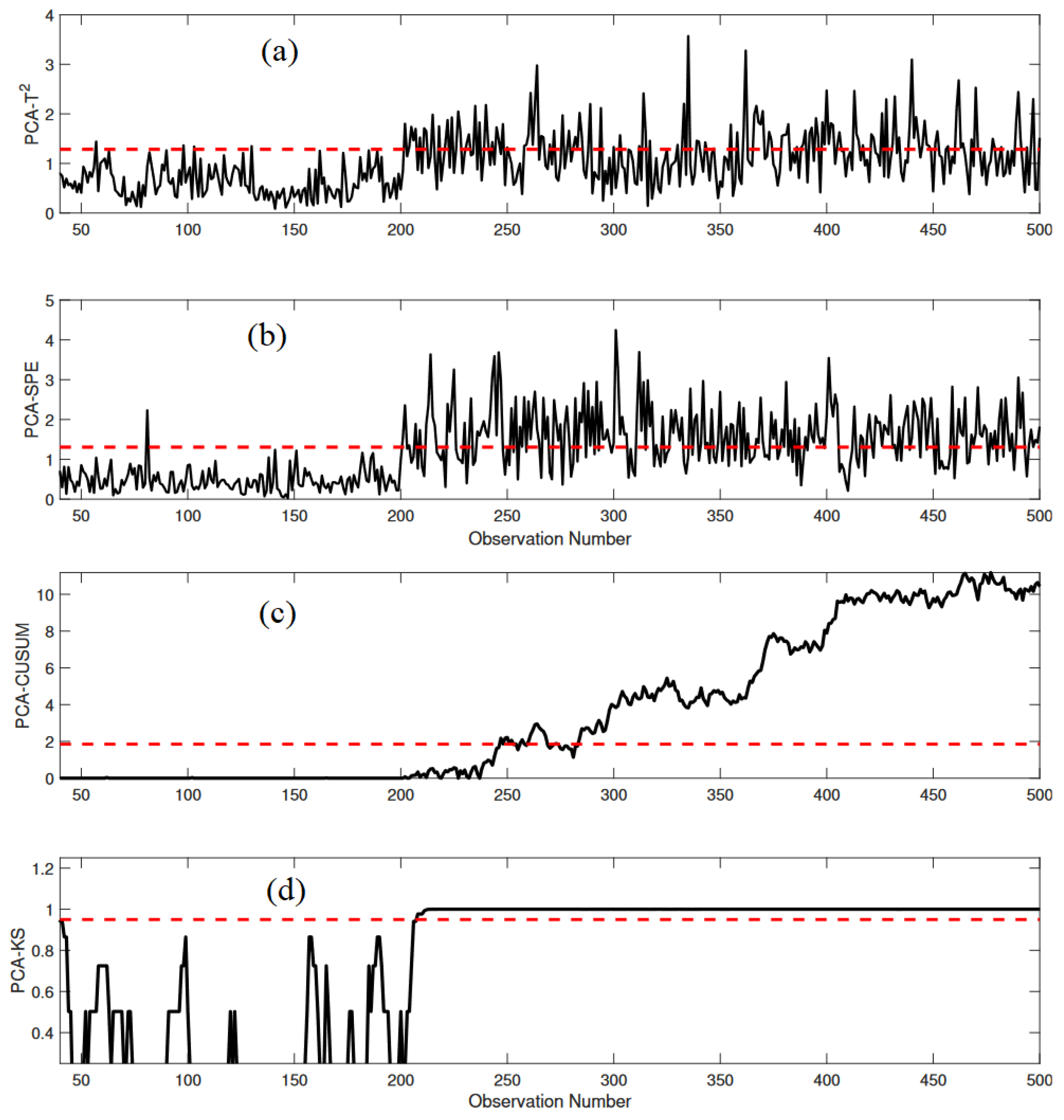
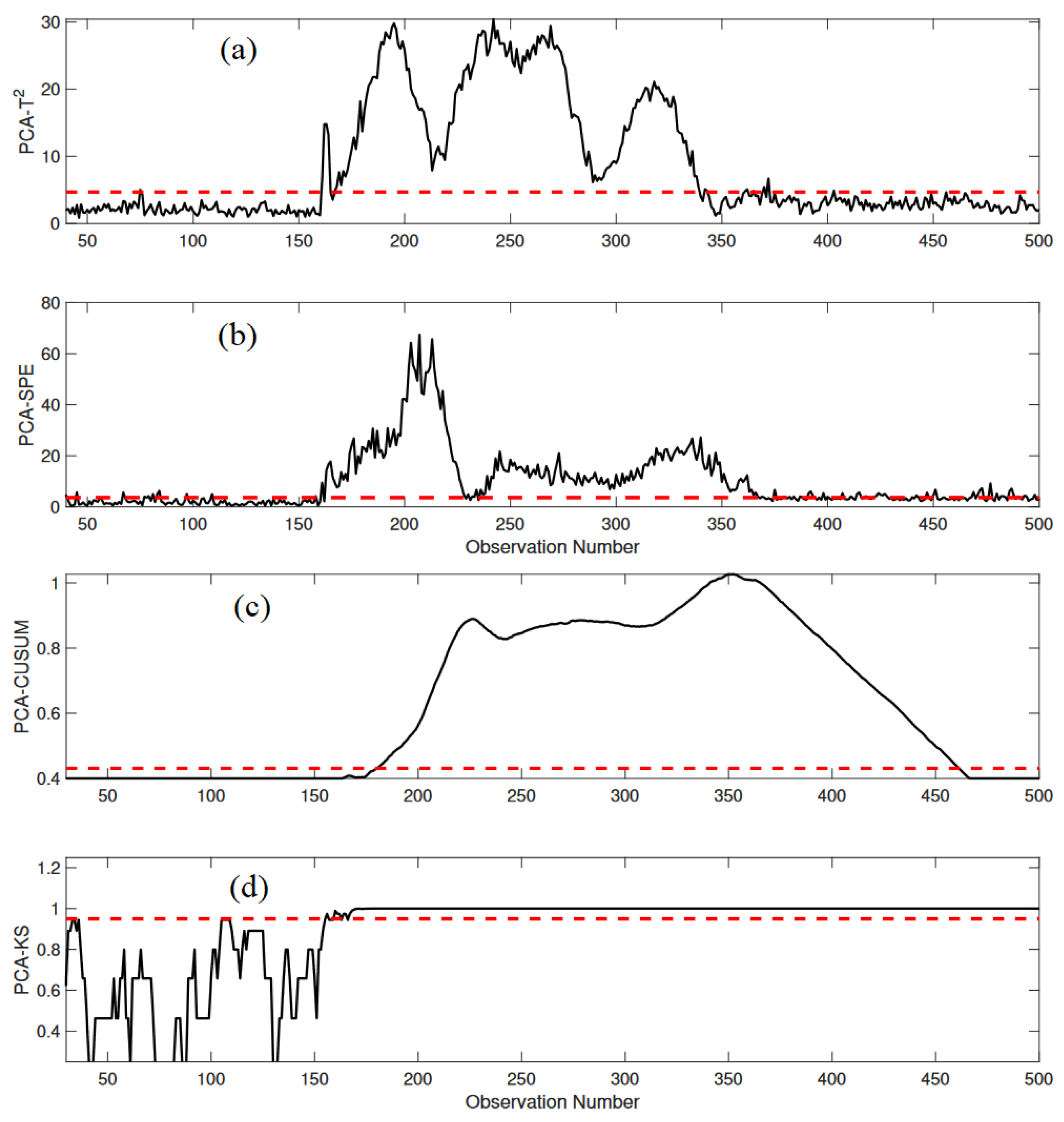
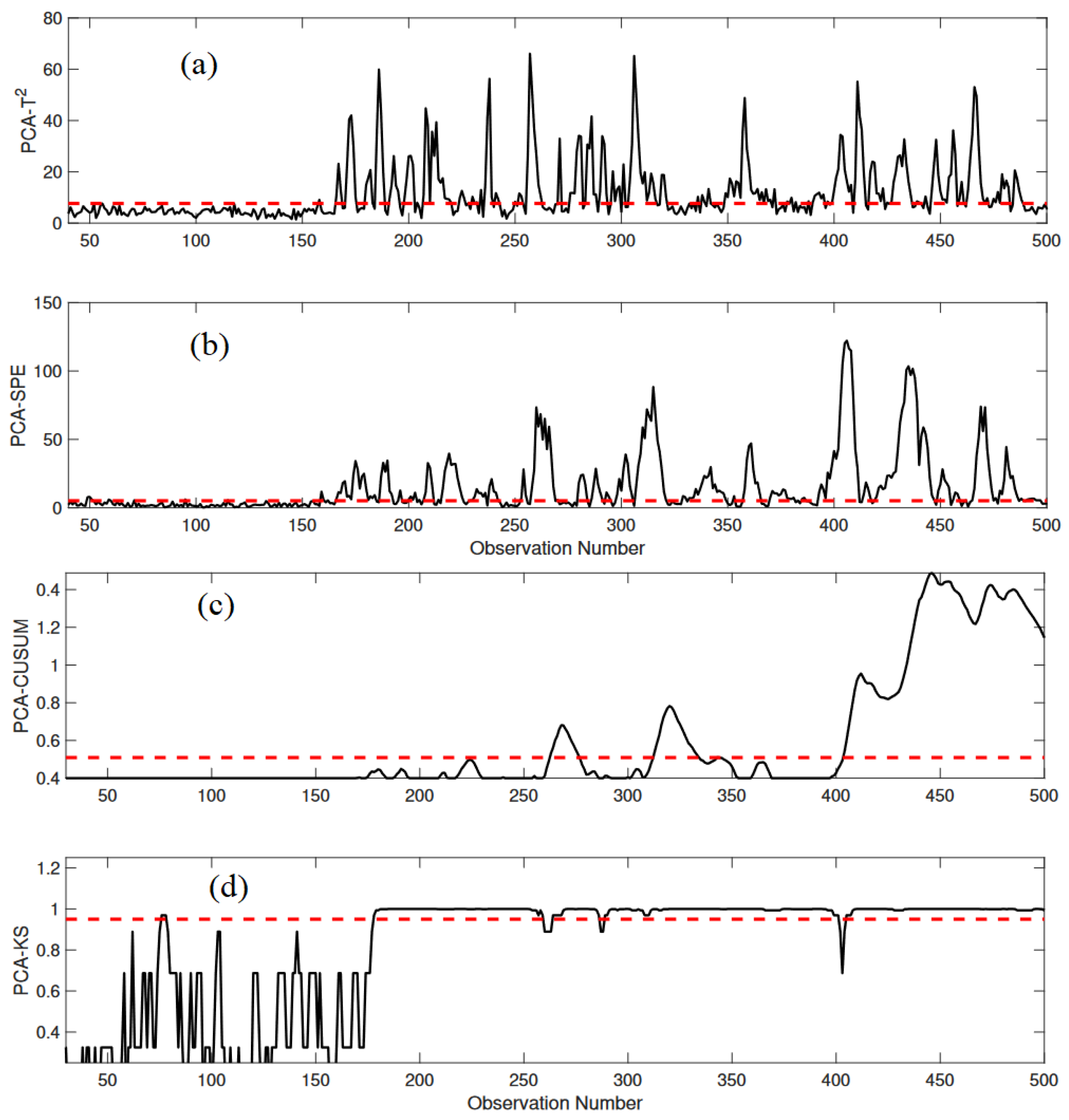
• The proposed PCA–KS approach is validated using both a simulated Plug-Flow Reactor (PFR) process and the Tennessee Eastman (TE) process. The evaluation involves various types of faults, including sustained bias faults, intermittent faults, and drift faults. Additionally, the performance of PCA–KS is compared with established techniques, such as PCA-T2, PCA-SPE, and PCA-CUSUM, ensuring a fair and accurate assessment. To quantitatively evaluate the performance of the investigated methods, five statistical evaluation metrics are employed. The results demonstrate the promising capability of the PCA–KS approach, characterized by a high detection rate and reduced false alarms.

The remainder of the paper is presented as follows: Section 2 provides a formulation of one-sample and two-sample KS tests, the change point detection capability of the KS test, the conventional PCA FD strategy, and the block diagram representation of the PCA–KS FD strategy. Section 3 assesses the effectiveness of the proposed PCA–KS FD strategy through a simulated PFR process and the benchmark Tennessee Eastman process. Finally, Section 4 concludes the paper with a summary of the findings and also discusses the potential future research directions.

2. Methodology

This section briefly overviews conventional PCA, the basic idea of Kolmogorov–Smirnov (KS), and the proposed PCA–KS fault detection approach.

2.1. Fault Detection Based on PCA

PCA is a dimensionality reduction technique that reduces the high-dimensionality of multivariate data while preserving its essential information. Its ability to transform complex data into a reduced-dimensional space and evaluate fault indicators has made it a cornerstone in anomaly detection across various industrial sectors [36]. In this section, the concept of PCA-based fault detection is presented, providing an in-depth understanding of its key components and operational principles.

Consider a dataset, $\mathbf{X}$$\in {\mathbb{R}}^{n\times m}$, where n represents the number of observations and m signifies the variables collected from a process plant. Each observation is stored as a vector, ${\mathbf{x}}_{\mathbf{i}}$ in ${\Re }^m$, and the dataset, $\mathbf{X}$, can be structured as $\mathbf{X}=[{\mathbf{x}}_{\mathbf{1}}^T,\dots ,{\mathbf{x}}_{\mathbf{n}}^T]$. Before applying PCA, the dataset is typically normalized to ensure that all variables have the same scale. After normalization, PCA is implemented to model the data, transforming it into a new space, ${\mathbf{X}}_{\mathbf{sc}}$, represented as

$${\mathbf{X}}_{\mathbf{sc}}={\mathbf{TV}}^{\mathbf{T}},$$

(1)

where $\mathbf{T}=[t_1,t_2,\dots ,t_m]$ are the score vectors and $\mathbf{V}=[v_1,v_2,\dots ,v_m]$ are the loading vectors.

Following PCA modeling, a subset of Principal Components (PCs) is selected to capture the most significant variance in the data. This selection is often guided by the Cumulative Percentage Variance (CPV) method [42]. The PCA model is then expressed as the sum of an approximated matrix, ${\widehat{\mathbf{X}}}_{\mathbf{sc}}$, and a residual matrix, F:

$${\mathbf{X}}_{\mathbf{sc}}=\widehat{\mathbf{T}}{\widehat{\mathbf{V}}}^{\mathbf{T}}+\tilde{\mathbf{T}}{\tilde{\mathbf{V}}}^{\mathbf{T}}={\widehat{\mathbf{X}}}_{\mathbf{sc}}+\mathbf{F}.$$

(2)

The matrices ${\widehat{\mathbf{X}}}_{\mathbf{sc}}$ and F contain vital information about the process, and fault detection relies on evaluating these components. This evaluation is facilitated through two key fault indicators: the $T^2$ statistic and the Squared Prediction Error (SPE) statistic. The $T^2$ statistic measures variations within the first p PCs of the PCA model and is defined for new data, $X_{new}$, as

$${\mathit{T}}^2={{\mathbf{X}}_{\mathbf{new}}}^T\widehat{\mathbf{V}}{\widehat{\Lambda }}^{-1}{\widehat{\mathbf{V}}}^T{\mathbf{X}}_{\mathbf{new}}.$$

(3)

The SPE statistic quantifies variations in the remaining m-p PCs and is expressed as

$$\mathit{SPE}={{\mathbf{X}}_{\mathbf{new}}}^T(\mathbf{I}-\widehat{\mathbf{V}}{\widehat{\mathbf{V}}}^{\mathbf{T}}){\mathbf{X}}_{\mathbf{new}}.$$

(4)

In the context of fault detection, if both the $T^2$ and SPE fault indicators exceed predefined threshold limits, it indicates the presence of a fault [43]. This dual-indicator approach is highly effective in detecting anomalies and deviations from normal operating conditions.

The calculation of detection thresholds for $T^2$ and SPE is based on the assumption that data are Gaussian distributed [43]. However, this may not always hold true in practice, especially in complex system, such as chemical engineering processes [44]. To address this limitation, alternative methods and robust statistical techniques may be employed. It is important to consider the specific characteristics of the data and the nature of the process when choosing an appropriate statistical model or distribution for threshold calculations. Additionally, non-parametric methods, such as the Kolmogorov–Smirnov test, which does not assume a particular distribution, can be valuable when the data distribution is uncertain or non-Gaussian.

2.2. Kolmogorov–Smirnov-Based Fault Indicator

The Kolmogorov–Smirnov test, often termed the KS test, is a powerful non-parametric statistical method used to assess the similarity between two distributions. It is particularly valuable when there is a need to determine if a set of data points conforms to a specified reference distribution. Unlike some parametric tests that assume specific distribution characteristics, the KS test does not make such assumptions. This non-parametric nature makes it versatile and robust, as it can be applied to a wide range of data distribution types.

The task of fault detection involves making a binary decision based on the comparison between current measurements and previous fault-free data. It requires a straightforward Yes or No determination regarding the presence of faults in a monitored process. To enhance this fault detection process, the potential of employing the non-parametric KS test is explored. The KS test is a member of the non-parametric statistical tests that do not rely on any specific assumptions about the data’s underlying distribution [45]. It is utilized to determine if the elements of a given probability distribution belong to a reference distribution. This non-parametric characteristic makes KS tests more robust and adaptable to a wide range of data distributions. The comparison is made by considering the Cumulative Distribution Function (CDF) of the two distributions or populations, leading to an appropriate conclusion.

When dealing with a dataset, the goal is often to determine the likelihood that the data sample follows a predefined distribution. In other cases, there might be two different data samples, and the aim is to assess the probability that they originate from the same distribution. For a Probability Distribution Function (PDF) denoted as F and applicable on the real number axis, R, the distribution function of a random variable, Y, is defined as $F\left(y\right)=Pr(\mathbf{Y}\le y)$. Given real numbers ${\mathbf{y}}_{\mathbf{1}}$, ${\mathbf{y}}_{\mathbf{2}}$ …${\mathbf{y}}_{\mathbf{n}}$, where n represents the number of observations within $F\left(y\right)$, the Empirical Cumulative Distribution Function (ECDF) is formulated as follows [46]:

$$F_n\left(y\right)={Pr}_n(\mathbf{Y}\le \mathbf{y})=\frac{1}{n}\sum _{i=1}^n\mathbf{I}(\mathbf{Y}\le \mathbf{y}),$$

(5)

where function I serves as an indicator. When the dataset values are arranged in ascending order of magnitude, the empirical distribution function can be represented as

$$F_n\left(y\right)=\left\{\begin{array}{cc}0\hfill & \mathbf{Y}<{\mathbf{y}}_{\mathbf{1}}\hfill \\ \frac{1}{n}\hfill & {\mathbf{y}}_{\mathbf{i}}\le \mathbf{Y}\le {\mathbf{y}}_{\mathbf{i}+\mathbf{1}}\hfill \\ 1\hfill & \mathbf{Y}\ge {\mathbf{y}}_{\mathbf{1}}\hfill \end{array}\right.$$

(6)

Now, consider the problem of assessing whether ${\mathbf{y}}_{\mathbf{1}}$, ${\mathbf{y}}_{\mathbf{2}}$ …${\mathbf{y}}_{\mathbf{n}}$ of $F_n\left(y\right)$ conform to a predetermined distribution function, $F\left(y\right)$. This scenario is formulated as a hypothesis test:

$$\begin{array}{c}\hfill H_0:F_n\left(y\right)=F\left(y\right)\\ \hfill H_1:F_n\left(y\right)\ne F\left(y\right)\end{array}$$

(7)

In this context, the null hypothesis, ${\mathit{H}}_{\mathit{0}}$, posits that the samples from the distribution, $F_n\left(y\right),$ are derived from the distribution, $F\left(y\right)$, while the alternative hypothesis, ${\mathit{H}}_{\mathit{1}}$, suggests otherwise. According to the law of large numbers in statistics, for any fixed point, $y\in \mathit{R}$:

$$\begin{array}{c}\hfill F_n\left(y\right)=\frac{1}{n}\sum _{i=1}^n\mathbf{I}(\mathbf{Y}\le \mathbf{y})⟶E\mathbf{I}(\mathbf{Y}\le \mathbf{y})=\\ \hfill Pr(\mathbf{Y}\le \mathbf{y})=F\left(y\right)\end{array}$$

(8)

The proportion of the sample within the set, $(-\infty ,y]$, approximates the probability of the set. Importantly, this approximation holds true across all values of $x\in \mathit{R}$, as demonstrated by Equation (9):

$$\underset{y\in \mathit{R}}{sup}(F_n\left(y\right)-F\left(y\right))⟶0$$

(9)

This expression signifies that the largest difference between $F_n\left(y\right)$ and $F\left(y\right)$ converges to 0. It is noteworthy that when $F\left(y\right)$ represents a continuous distribution, the distribution defined in Equation (9) becomes independent of the specific distribution, F. This property further solidifies the robustness of the KS test. An essential step in the KS test involves defining the inverse of $F\left(y\right)$ as [47]

$$F^{-1}\left(z\right)=min\{y:F\left(y\right)\ge z\}$$

(10)

This definition can be alternatively expressed as

$$\begin{array}{c}\hfill Pr(\underset{y\in \mathit{R}}{sup}|(F_n\left(y\right)-F\left(y\right))|\le t)=Pr(\underset{0\le z\le 1}{sup}|F_n\left(F^{-1}\left(z\right)\right)-z|\le t)\end{array}$$

(11)

Utilizing the definition of the empirical CDF, $F_n$, the relationship between $F_n\left(F^{-1}\left(z\right)\right)$ and $F_n\left(y\right)$ can be established as follows [48]:

$$\begin{array}{c}\hfill F_n\left(F^{-1}\left(z\right)\right)=\frac{1}{n}\sum _{i=1}^n\mathbf{I}({\mathbf{Y}}_{\mathbf{i}}\le F^{-1}\left(z\right))=\frac{1}{n}\sum _{i=1}^n\mathbf{I}(F\left(Y_i\right)\le z)\end{array}$$

(12)

This equivalence shows how the empirical CDF is constructed using the indicator function, effectively capturing the distribution characteristics. The next step is to relate the probability of the supremum of $|F_n\left(F^{-1}\left(z\right)\right)-z|$ to the probability of the supremum of $|\frac{1}{n}{\sum }_{i=1}^n\mathbf{I}(F\left(Y_i\right)\le z)-z|$, as indicated below [48]:

$$\begin{array}{c}\hfill Pr(\underset{0\le z\le 1}{sup}|F_n\left(F^{-1}\left(z\right)\right)-z|\le t)=Pr(\underset{0\le z\le 1}{sup}|\frac{1}{n}\sum _{i=1}^n\mathbf{I}(F\left(Y_i\right)\le z)-z|\le t)\end{array}$$

(13)

It is worth noting that the distribution of $F\left(Y_i\right)$ follows a uniform distribution on the interval [0, 1], supported by the property that the CDF of $F\left(Y_1\right)$ is expressed as [49]

$$Pr(F\left(Y_1\right)\le t)=Pr(F\left(Y_1\right)\le F^{-1}\left(t\right))=F\left(F^{-1}\left(t\right)\right)=t$$

(14)

As a result, the random variables in $F\left(Y_i\right)$ for $i\le n$ are independent and exhibit a uniform distribution on the interval [0, 1]. This independence from the specific distribution, F, emphasizes the universality and robustness of the Kolmogorov–Smirnov test. From this comprehensive analysis, the Kolmogorov–Smirnov statistic is formally defined as [50]

$$D_n=ma{x}_{-\infty <x<\infty }\mid F_n\left(y\right)-F\left(y\right)\mid .$$

(15)

The Glivenko–Cantelli theorem is crucial in interpreting the Kolmogorov–Smirnov statistic, denoted as $D_n$. According to this theorem, as the sample size, n, approaches infinity ($n\to \infty$), $D_n$ tends to zero, signifying the convergence of the empirical distribution, $F_n\left(y\right)$, towards the known distribution, $F\left(y\right)$ [51]. In essence, when the number of data points is sufficiently large, the empirical distribution of the sample closely aligns with the distribution function of the known distribution. The Kolmogorov–Smirnov test demonstrates remarkable consistency in accepting the null hypothesis, $H_0$, which postulates that the elements in $F_n\left(y\right)$ originate from the distribution, $F\left(y\right)$. This test’s consistency against various alternatives underlines its robustness and reliability [52]. In Equation (15), a deviation of the Kolmogorov–Smirnov statistic, $D_n$ from zero, resulting in a larger value, implies the rejection of the null hypothesis. This rejection indicates that the samples comprising $F_n\left(y\right)$ do not conform to the distribution represented by $F\left(y\right)$. The ECDF of $F_n\left(y\right)$ closely mirrors the ECDF of $F\left(y\right)$ when $D_n$ equals zero. Conversely, when $D_n$ deviates from zero, it introduces a noticeable discrepancy between the ECDF of $F_n\left(y\right)$ and that of $F\left(y\right)$, as depicted in Figure 1 to illustrate this distinction between similar and dissimilar distributions.

Expanding on the Kolmogorov–Smirnov test, the test can be extended into a two-sample KS test, which is especially useful in fault detection applications where the goal is to compare data from normal and faulty conditions. This scenario often arises in industrial processes or system monitoring. In such cases, the interest lies in evaluating whether the observations $y_{a1},y_{a2},\dots ,y_{n_a}$ from distribution $G\left(y\right)$ match those of $y_{b1},y_{b2},\dots ,y_{n_b}$ from distribution $H\left(y\right)$. To quantify the disparity between the ECDFs of these two distributions, the KS statistic is employed, denoted as $D_{stat}$, which is defined as the maximum absolute difference between $G_{n_a}\left(y\right)$ and $H_{n_b}\left(y\right)$ [46].

$$D_{stat}=ma{x}_{-\infty <y<\infty }\mid G_{n_a}\left(y\right)-H_{n_b}\left(y\right)\mid$$

(16)

To facilitate direct probability calculations, the KS statistic, $K{S}_{stat}$, is computed and defined as

$$K{S}_{stat}=Pr\left(D_{stat}\right)=1-Q_{KS}\left(\lambda \right).$$

(17)

Here, $\lambda$ is determined as

$$\lambda =\left(\sqrt{ED}+0.12+{\displaystyle \frac{0.11}{\sqrt{ED}}}\right),$$

(18)

where $ED$ is the effective sample size, calculated as

$$ED={\displaystyle \frac{n_a{n}_b}{n_a+n_b}},$$

(19)

where $n_a$ and $n_b$ represent the number of observations in $G\left(y\right)$ and $H\left(y\right)$, respectively. The expression in Equation (17) provides a reliable approximation, particularly for small to medium values of $ED$. In scenarios where $y_{a1},y_{a2},\dots ,y_{n_a}$ are independent and identically distributed with continuous empirical CDF $G\left(y\right)$, and $y_{b1},y_{b2},\dots ,y_{n_b}$ are independent and identically distributed with continuous empirical CDF $H\left(y\right)$, the KS distribution function, $Q_{KS}\left(\lambda \right)$, can be expressed as [50]

$$Q_{KS}\left(\lambda \right)=2\sum _{i=1}^{\infty }{(-1)}^{i-1}{exp}^{-2i^2{\lambda }^2}.$$

(20)

The expression in Equation (20) represents a monotonic function with limiting values, 1 as $\lambda$ approaches 0 and 0 as $\lambda$ tends towards infinity, allowing us to evaluate the significance of the test result.

$$\delta =\left\{\begin{array}{ccc}\hfill 1& \hfill :& \lambda \to 0\hfill \\ \hfill 0& \hfill :& \lambda \to \infty \hfill \end{array}\right.$$

Figure 2 visually represents the computation of the KS statistic between two distributions within a moving window. The probability, $Q_{KS}$, obtained from the KS statistic is a useful indicator of the similarity between two distributions. If the distributions are similar, then the probability, $Q_{KS}$, approaches 1. Contrarily, if the distributions are dissimilar, $Q_{KS}$ tends to be closer to 0. In industrial process monitoring and fault detection, statistical indicators are often compared to predefined threshold values to make decisions regarding potential faults. This is typically done at a significance level, often set to $\alpha =0.95$ or $\alpha =0.99$. If the calculated $K{S}_{stat}$ is less than $\alpha$, it signifies that the null hypothesis, $H_0$, is accepted, suggesting that the empirical CDFs of both distributions are equal. Conversely, if $K{S}_{stat}$ is greater than $\alpha$, the alternative hypothesis, $H_1$, is accepted, indicating that the empirical CDFs of the two distributions are not equal [53]. In this study, the KS test is employed for fault detection applications. Since fault detection often involves comparing two datasets (fault-free and faulty data) to determine the presence or absence of a fault, the KS test presents a robust and efficient tool for enhancing fault detection performance. Leveraging the KS test enables robust evaluation of deviations between datasets, contributing to improved reliability and accuracy in fault detection. This approach is particularly valuable in industrial and engineering settings where the consequences of missed faults can be significant.

In summary, the main steps of the KS-based fault detection approach are summarized as follows:

• Data Collection: Gather data from the system or process that you want to monitor and detect faults in.
• Data Preprocessing: Prepare the collected data for analysis. This step may involve data cleaning, normalization, and transformation to ensure that it is suitable for the KS-based fault detection approach.
• Select Reference Data: Choose a dataset or set of observations representing normal or fault-free operation. This reference dataset will serve as a baseline for comparison.
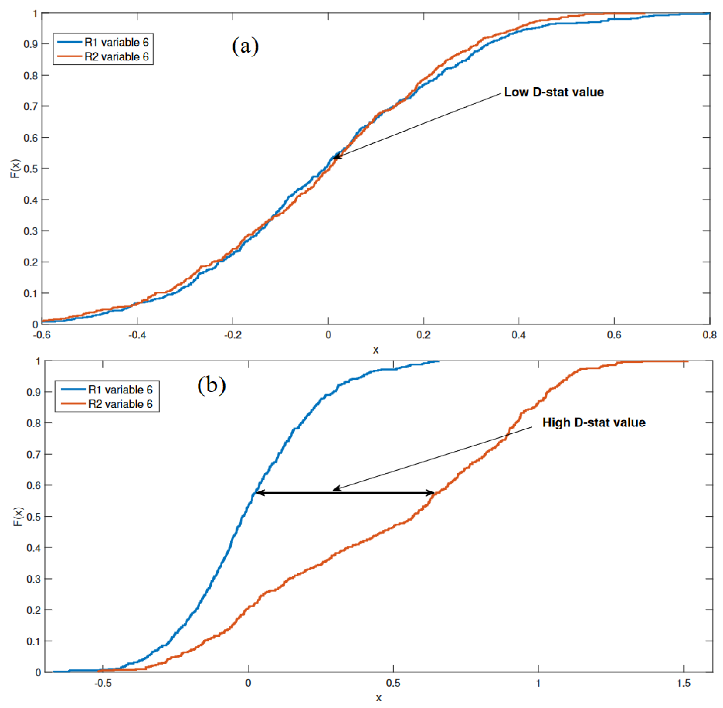
• Calculate Empirical CDFs: Compute the Empirical Cumulative Distribution Functions (ECDFs) for both the reference data and the incoming data stream. These ECDFs represent the distribution of the data in both cases.
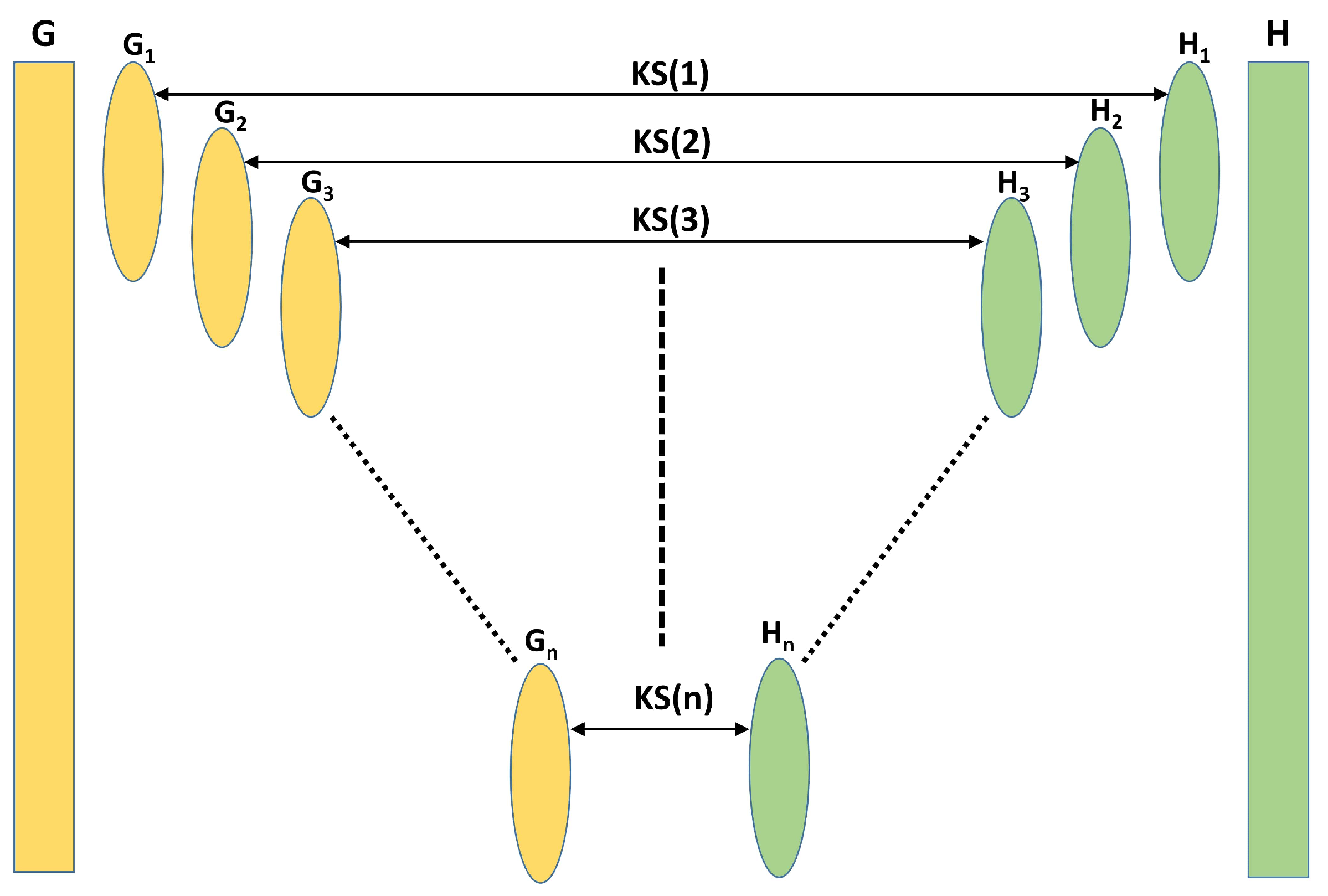
• Apply the KS Test: Use the Kolmogorov–Smirnov (KS) test to compare the two ECDFs. The KS test will quantify the maximum difference (KS statistic) between the two distributions.
• Threshold Setting: Define a threshold value or critical value for the KS statistic. This threshold will determine when a fault is detected. If the KS statistic exceeds this threshold, it indicates a significant difference between the two distributions.
• Monitoring in a Moving Window: Implement a moving window approach to continuously monitor the incoming data stream. The window moves over time, and at each step the KS statistic is computed for the data within the window.
• Fault Detection: Compare the computed KS statistic with the predefined threshold in the moving window. If the KS statistic exceeds the threshold, it suggests a fault or anomaly in the data.

2.3. The PCA–KS-Based Fault Detection Strategy

In this section, the proposed fault detection strategy is introduced, combining PCA, a multivariate method, with the Kolmogorov–Smirnov non-parametric test. This fusion leads to an efficient PCA–KS-based FD strategy aimed at effectively and efficiently detecting faults in multivariate processes. The strategy revolves around the computation of the KS statistic using residuals generated from normal operating data and new online data, focusing on using a moving window to enhance detection capabilities. The foundation of the PCA–KS strategy lies in constructing a reference PCA model using normal operating data, denoted as X. This model captures the underlying patterns and behaviors of the system under normal conditions. The first step in this strategy involves generating residuals, represented as E, according to the following expression [36]:

$$\mathbf{E}=\mathbf{X}-\widehat{\mathbf{X}}=\mathbf{X}-{\mathbf{XVV}}^{\mathbf{T}}.$$

(21)

where $\widehat{\mathbf{X}}$ is the approximation of the original data, $\mathbf{V}$, and contains the loading vectors. It is crucial to note that the KS test compares two distributions or signals, which are represented in vector form (either as a row or column vector). Consequently, once residuals are generated for both datasets, their norm values are computed to create the respective column vectors for the KS test, enabling the accurate detection of deviations from normal operating conditions. The proposed PCA–KS-based fault detection strategy is illustrated in Figure 3.

The main steps of the proposed PCA–KS strategy are outlined in Algorithm 1.

Algorithm 1: PCA–KS-based Fault Detection Strategy

Offline Stage: Obtain data at normal operating conditions—$X_{train}$. Scale $X_{train}$ to mean of zero and unity variance. Construct a reference PCA model using $X_{train}$ and generate the residuals—RC. Take the norm of RC to generate $\mathbf{C}\in {\Re }^{n\times 1}$. Online Stage: Obtain online data—$X_{test}$. Scale $X_{test}$ to have a mean of zero and unity variance. From the reference PCA model parameters, generate the residuals—RD. Take the norm of RD to generate $\mathbf{D}\in {\Re }^{n\times 1}$. Compute the KS statistic between C and D using the computation presented in Figure 2. If the KS statistic is greater than the significance level $\alpha$, declare a fault.

The performance of the PCA–KS-based FD strategy is closely linked to the choice of the moving window size. By employing a moving window, the non-parametric test demonstrates enhanced precision and robustness in the presence of smaller datasets. The selection of an appropriate moving window size, denoted as j, is adaptable based on the characteristics of the process data. It is crucial to note that the KS test is conducted by comparing two distributions or signals, which are represented in vector form (either as a row or a column vector). Consequently, once residuals are generated for both datasets, their norm values are computed to create the respective column vectors for the KS test, enabling the accurate detection of deviations from normal operating conditions.

The fault detection methods considered in this study will be evaluated using several statistical metrics: the Fault Detection Rate (FDR), False Alarm Rate (FAR), precision, recall, and F1-score. For a binary detection task, the evaluation metrics are computed using the number of True Positives (TP), False Positives (FP), False Negatives (FN), and True Negatives (TN) and are presented as follows. They are especially useful for binary detection tasks where a clear distinction between normal and fault conditions is essential.

• Recall (Sensitivity): Recall, often referred to as sensitivity, measures the ability of an FD strategy to correctly identify true positive cases [54].

  $$\mathrm{Recall}=\frac{\mathrm{TP}}{\mathrm{TP}+\mathrm{FN}}$$

  (22)
  Recall provides insights into the strategy’s ability to detect actual faults when they occur, minimizing the chances of missing any real issues.
• Precision: Precision evaluates the precision and accuracy of an FD strategy in correctly detecting true positive cases [54].

  $$\mathrm{Precision}=\frac{TP}{TP+FP}$$

  (23)
  Precision is valuable for assessing the strategy’s reliability in avoiding false alarms, ensuring that when it signals a fault, it is highly likely to be a real issue.
• F1-Score: The F1-score is a harmonic mean of precision and recall. It balances these two metrics, making it a useful overall performance indicator. The F1-score is calculated as follows [54]:

  $$\mathrm{F}1\text{-}\mathrm{Score}=\frac{2·\mathrm{Precision}·\mathrm{Recall}}{\mathrm{Precision}+\mathrm{Recall}}=\frac{2TP}{2TP+FP+FN}$$

  (24)
  The F1-score takes both false alarms and missed faults into account, providing a holistic view of the strategy’s performance. It helps in achieving a balance between precision and recall, ensuring that the FD strategy is effective in both detecting true faults and avoiding false alarms.

3. Results and Discussion

This section will focus on evaluating the performance of the proposed PCA–KS-based fault detection strategy using data from two multivariate processes, the PFR process and the TE process. The proposed strategy will be compared against PCA-$T^2$, PCA-SPE, and PCA-CUSUM-based fault strategies.

3.1. Plug Flow Reactor

In this section, the performance of the proposed fault detection strategy is assessed by its ability to identify different faults in the Plug Flow Reactor process.

3.1.1. Modeling and Data Description

In chemical engineering, the Plug Flow Reactor (PFR) is a fundamental device used in various chemical processes, especially in gas–liquid phase reactions, both exothermic and endothermic. Its performance significantly influences the yield of the desired product. The PFR forms a hollow cylindrical tube or pipe through which reactants flow as they undergo a chemical transformation. Its significance is prominent in numerous chemical processing industries where controlled reactions are crucial for producing desired products. One of the key characteristics of the PFR is its unique flow pattern. Unlike other reactor types, the PFR is designed to minimize axial mixing, resulting in a flow pattern with a nearly constant velocity profile. This means that, as reactants move through the reactor, they experience minimal cross-mixing along its length. Instead, the concentration of reactants changes primarily along the axial direction of flow. Figure 4 illustrates a schematic of a typical Plug Flow Reactor. In this representation, the PFR is depicted as a cylindrical tube, typically wrapped around an acrylic mold, and encased in a tank. This configuration helps maintain temperature control within the reactor, a critical factor in many chemical processes.

In the PFR system, a coolant is circulated through the annular space of the reactor to control its temperature. The chosen reaction system involves two first-order reactions occurring in series. Reactant A produces product B, which decomposes to form product C. The desired product from this reaction system is B. Several temperature sensors are strategically placed within the reactor to monitor temperatures at different locations. The following reactions describe the dynamic PFR model [11]:

$$A\to B\to C$$

(25)

The mathematical representation of the Partial Differential Equations (PDEs) governing the PFR process is as follows:

$$\frac{\partial C_A}{\partial t}=-v_1\frac{\partial C_A}{\partial x}-k_{10}{e}^{-E_1/R{T}_r}{C}_A$$

(26)

$$\frac{\partial C_B}{\partial t}=-v_1\frac{\partial C_B}{\partial x}+k_{10}{e}^{-E_1/R{T}_r}{C}_A-k_{20}{e}^{-E_2/R{T}_r}{C}_B$$

(27)

$$\begin{array}{c}\hfill \frac{\partial T_r}{\partial t}=-v_1\frac{\partial T_r}{\partial x}+\frac{\Delta H_{r_1}}{{\rho }_m{c}_{pm}}{k}_{10}{e}^{-E_1/R{T}_r}{C}_A+\\ \hfill \frac{\Delta H_{r_2}}{{\rho }_m{c}_{pm}}{k}_{20}{e}^{-E_2/R{T}_r}{C}_B+\frac{U_w}{{\rho }_m{c}_{pm}{V}_r}[T_j-T_r]\end{array}$$

(28)

$$\frac{\partial T_j}{\partial t}=-u\frac{\partial T_j}{\partial x}+\frac{U_{wj}}{{\rho }_{mj}{c}_{pmj}{V}_j}[T_r-T_j]$$

(29)

In these equations, various parameters and variables are defined as follows: u represents the flow rate of the heating fluid in the jacket, $C_A$ and $C_B$ are the concentrations of reactants A and B, $T_r$ and $T_j$ are the temperatures of the fluid in the reactor and jacket, $\Delta H_{r_1}$ and $\Delta H_{r_2}$ represent the enthalpies of the reactions in Equation (25), ${\rho }_m$ is the density of the fluid in the reactor, ${\rho }_{mj}$ is the density of the fluid in the jacket, $c_{pm}$ and $c_{pmj}$ are the heat capacities of the fluid in the reactor and jacket, $v_r$ and $v_j$ are the volumes of the reactor and jacket, $U_w$ and $U_{wj}$ are the heat transfer coefficients of the reactor and jacket, $k_{10}$ and $k_{20}$ are Arrhenius constants, and $E_1$ and $E_2$ are the activation energies of the reactions.

The data are generated by perturbing the input flow rate of the reaction feed around the steady-state nominal values presented in

Table 1. Model parameters of the Plug Flow Reactor process.

Process Variable	Description	Value/Unit
$v_l$	Flow rate of reactant	1 m/min
u	Flow rate of heating fluid in jacket	0.5 m/min
$C_A$	Concentrations of reactant A	4 mol/L
$C_B$	Concentrations of reactant B	0 mol/L
$T_r$	Temperature of fluid in reactor	320 K
$T_j$	Temperature of fluid in jacket	375 K
$\Delta H_{r_1}$	Enthalpy of dynamic reaction in Equation (25)	0.5480 kcal/kmol
$\Delta H_{r_2}$	Enthalpy of dynamic reaction in Equation (25)	0.9860 kcal/kmol
${\rho }_m$	Density of fluid in the reactor	0.09 kg/L
${\rho }_{mj}$	Density of fluid in the jacket	0.10 kg/L
$c_{pm}$	Heat capacity of fluid in the reactor	0.231 kcal/(kg K)
$c_{pmj}$	Heat capacity of fluid in the jacket	0.80 kcal/(kg K)
$V_r$	Volume of the reactor	10 lt
$V_j$	Volume of the jacket	8 lt
$U_w$	Heat transfer coefficient of the reactor	0.20 kcal/(min K)
R	Gas constant	1.987 kcal/(min K)
$k_{10}$	Arrhenius constant	$5.0\times {10}^{12}$ min${}^{-1}$
$k_{20}$	Arrhenius constant	$5.0\times {10}^2$ min${}^{-1}$
$E_1$	Activation enegy of reaction in Equation (25)	20,000 kcal/kmol
$E_2$	Activation enegy of reaction in Equation (25)	50,000 kcal/kmol

. The flow input is perturbed around the nominal operating point with a Pseudo-Random Binary Signal (PRBS) in the frequency range of [0, 0.05 ${\omega }_n$], where ${\omega }_n=\pi /T$ represents the Nyquist frequency. The dataset consists of 1000 measurements and includes 11 variables: the input flow rate, nine temperatures from different locations in the reactor, and the product concentration. The data generated from the simulation are noise free. To replicate real industrial data measurements, noise with a Signal-to-Noise Ratio (SNR) of 20 is introduced into the data. The measurements are divided into two halves: 500 observations as training data and 500 observations as testing data. The 500 training observations are used to develop the PCA model. The PCA model is developed for the training data, with five optimal Principal Components (PCs) being selected. This developed model is then used to detect any possible faults in the testing data. In the case of the KS computation part, a moving window of size 30 is adopted.

One of the crucial parameters to monitor in the PFR is the temperature profile along its length. Several factors, such as the reaction conditions, heat transfer to the coolant, and feed flow rate, contribute to the dynamic nature of the temperature within the reactor. Maintaining an optimal temperature profile is paramount to achieving the desired product yield. Deviations from the ideal temperature can result in undesirable outcomes. Lower temperatures than required might lead to a lower product yield, affecting the overall production efficiency. Conversely, higher temperatures can create hot spots within the reactor, leading to catalyst deactivation and reactor shutdown, ultimately causing production and economic losses. In the context of temperature and concentration monitoring, the reliability of sensors becomes crucial. Accurate and reliable temperature readings, especially from sensors such as T5 and T6, play a pivotal role in timely adjustments to maintain the optimal conditions within the reactor. Any malfunction or discrepancy in sensor readings must be promptly detected, reported, and rectified to prevent process inefficiencies and potential economic losses. In addition to temperature, monitoring the concentration of the product, often measured as $C_B$, is equally significant. Product quality directly depends on the concentration levels, making accurate and consistent product concentration measurements crucial for ensuring the production of high-quality, desirable end products. In this study, temperature sensor faults are simulated to evaluate the performance of the investigated fault detection methods. In addition, concentration measurement plays a very important role in deciding the product’s quality, and malfunction in the product sensor results in heavy economic loss. Further, the detection of product concentration ($C_B$) sensor faults has been assessed in this study. This is important for both product quality and economic considerations.

3.1.2. Different Fault Scenarios

In this study, the proposed PCA–KS-based strategy is evaluated by introducing various simulated sensor faults. These faults include bias, drift, and intermittent types, providing a comprehensive assessment of the strategy’s performance.

• Bias Fault: A bias fault is a sudden and significant deviation in a variable’s behavior from its normal range. It can be mathematically expressed as

  $$S\left(t\right)=S_N\left(t\right)+b,$$

  (30)

  where $S_N\left(t\right)$ is the variable’s normal range and b represents the bias introduced at time, t. Bias faults are characterized by a pronounced and persistent shift in sensor readings.
• Drift Fault: Sensor drift is characterized by a gradual and exponential change in sensor readings over time. This phenomenon is attributed to the aging of the sensing element and can be mathematically defined as

  $$S\left(t\right)=S_N\left(t\right)+M(t-t_f),$$

  (31)

  where M denotes the slope of the drift and $t_f$ represents the time at which the fault begins. Drift faults are a consistent departure from normal behavior, growing progressively.
• Intermittent Fault: Intermittent sensor faults are marked by irregular intervals of appearance and disappearance. These faults are characterized by short instances of variation in sensor readings, typically in the form of small variations in the bias term, followed by a return to normal behavior.

Table 2. Simulated fault scenarios in Plug Flow Reactor process.

Fault Number	Description	Variable	Type of Fault
F1	Large step (3.5% of total variation)	Temperature T5	Bias
F2	Medium step (2% of total variation)	Temperature T5	Bias
F3	Small step (0.9% of total variation)	Temperature T5	Bias
F4	Multiple step (2% of total variation)	Temperature T6	Intermittent
F5	Ramp (Slope of 0.002)	Product concentration $C_B$	Drift

provides an overview of the various simulated fault scenarios employed to evaluate the performance of the fault detection strategy. Specifically, these scenarios include different faults introduced in the PFR process. In the case of the bias fault, the study has considered three distinct magnitudes of fault: a large step change, a medium step change, and a small step change. These fault scenarios have been applied to the temperature variable, T5, beginning from the 200th sampling instant and continuing until the end of the testing data. Notably, the simulated large step change (F1) manifests as a significant deviation from the normal behavior, accounting for 3.5% of the total variation. During this fault period, the statistical indicators employed by the fault detection strategy perform significantly well, with all indicators surpassing the established confidence threshold within the fault region. Notably, the $T^2$ and SPE-based indicators exhibit minimal false alarms, while the CUSUM and KS indicators effectively detect the fault without triggering any false alarms. Furthermore, the fault scenarios denoted as F2 and F3 represent medium and small step changes, constituting 2% and 0.9% of the total variation, respectively.

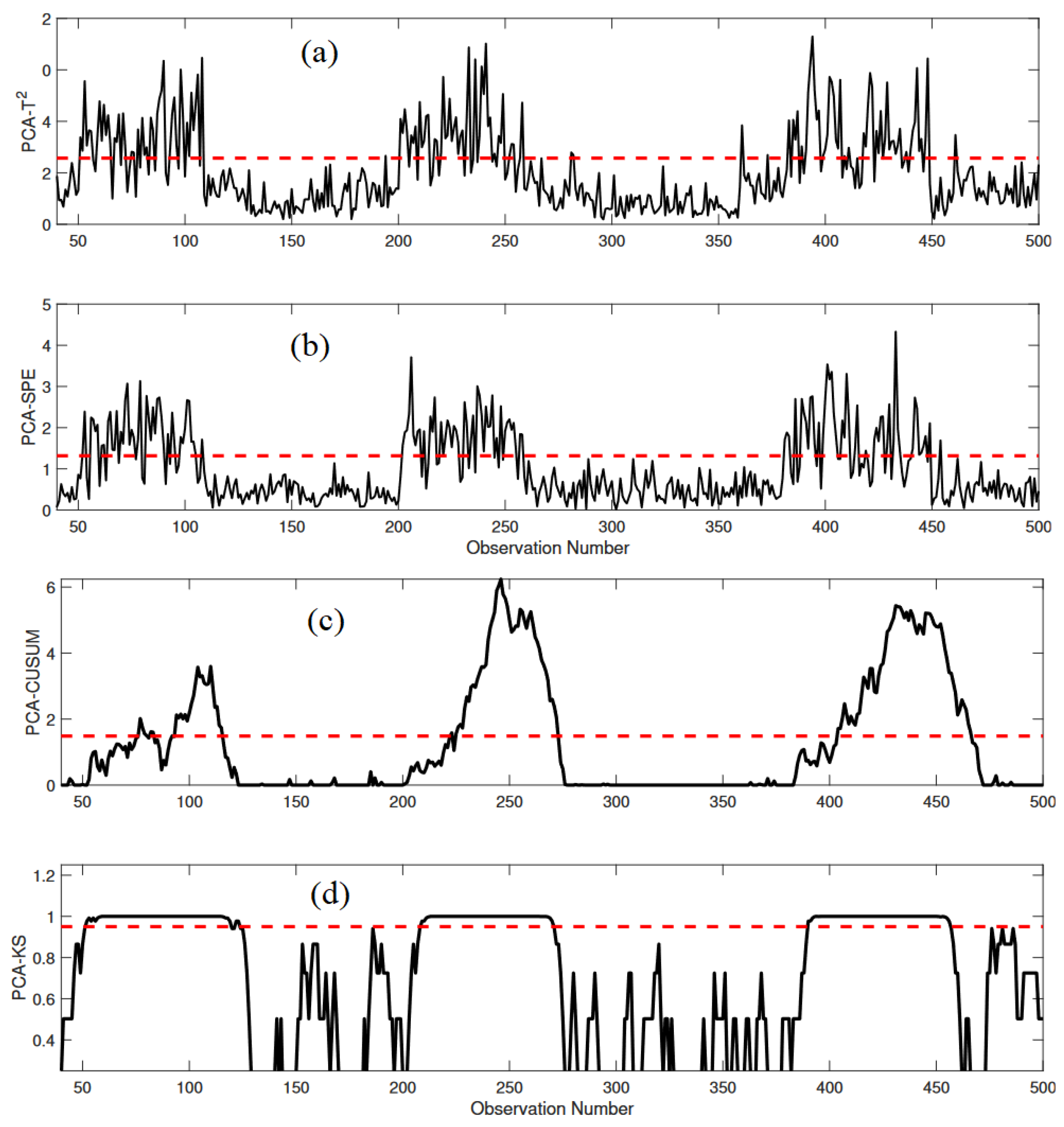
3.1.3. Monitoring Results

This section provides the results of the proposed FD strategy in monitoring different faults in the PFR process. First, the results of the four different fault detection approaches in identifying fault F2 are illustrated in Figure 5a–d. In the case of the $T^2$ indicator, it exhibits a robust and accurate fault detection performance with minimal instances of missed detections and false alarms, as depicted in Figure 5a. However, when considering the SPE indicator of PCA, it displays a comparatively higher number of missed detections and false alarms, as visualized in Figure 5b. Moving on to the CUSUM indicator, it showcases a relatively smooth fault detection profile, but a slight detection delay can be observed, as illustrated in Figure 5c. In contrast, the KS indicator surpasses the others by consistently remaining above the confidence limit within the fault region, achieving fault detection without any missed detections or significant detection delays. This is evident in Figure 5d, highlighting the distinct advantage of the KS indicator as a reliable fault detection method in this scenario.

The results of the four monitoring techniques in the presence of a sensor temperature fault (F3) with a small magnitude are presented in Figure 6a–d. Results reveal distinct differences in fault detection capabilities among the methods. In Figure 6a,b, both the $T^2$ and SPE statistics exhibit limited effectiveness in clearly detecting the fault. The responses from these indicators are somewhat unclear, failing to provide a robust detection of the fault’s onset and progression. This could be due to their decision statistics being solely based on the actual observations, making them insensitive to small changes in the system. These methods might require more significant deviations from the normal state to trigger a reliable alarm. The CUSUM fault indicator, as shown in Figure 6c, offers better performance compared to the $T^2$ and SPE statistics. This improved performance is due to its decision statistic considering all historical data, making it sensitive to small changes in the system. However, there is still a small delay in detecting the fault, suggesting that it may not be as timely in identifying such small-magnitude faults. Despite this delay, the CUSUM method demonstrates its capability to eventually detect the fault effectively. However, the KS indicator, displayed in Figure 6d, offers a highly accurate and timely fault detection, demonstrating a significant advantage in small-magnitude fault detection. The KS indicator detects the fault starting from the 205th sampling time instant with minimal delay. These results underscore the superiority of the PCA–KS FD strategy in detecting small-magnitude faults within a noisy process environment, with the KS indicator proving to be particularly adept in this regard.

The effectiveness of the PCA–KS-based FD strategy in monitoring fault F4, an intermittent fault, is presented in the following analysis (Figure 7a–d). This fault is introduced in temperature variable T9 during specific sampling time intervals, which include [50, 110], [200, 260], and [380, 450]. Figure 7a,b displays the response of the $T^2$ and SPE-based fault indicators in monitoring intermittent faults. Both the PCA-$T^2$ and PCA-SPE strategies fail to detect this abnormality effectively, as is evident from the monitoring plots. These indicators show limitations in their ability to accurately capture and identify the intermittent fault’s occurrences. In contrast, Figure 7c,d shows the response of the CUSUM and KS-based fault indicators in monitoring the intermittent fault. Both of these indicators demonstrate the capability to detect the fault. However, it is worth noting that the $T^2$ and SPE fault indicators have some missed detections, while the CUSUM indicator exhibits occasional false alarms. These characteristics are not indicative of a robust fault detection strategy. Conversely, the proposed PCA–KS method exhibits precise and sharp fault detection for fault F4, even in the presence of noise. This capability highlights the effectiveness of the PCA–KS-based strategy in detecting intermittent faults. The superiority of the PCA–KS-based fault strategy in detecting intermittent fault F4 is evident from its precise fault detection capability, even in the presence of noise. Intermittent faults, which can appear and disappear at irregular intervals, are often challenging to identify accurately, but the PCA–KS strategy excels. It effectively leverages the non-parametric nature of the KS statistic, sensitivity to distribution differences, and the moving window approach to detect faults promptly. This robust performance underscores the potential of the PCA–KS-based strategy to enhance fault detection in real-world processes and demonstrates its reliability even in noisy and dynamic industrial environments.

The monitoring results presented in Figure 8a–d reflect the performance of different fault indicators in detecting sensor aging fault F5, which exhibits a gradual drift. The sensor aging fault F5 is inserted at sampling time instant 200 in variable $C_B$. These results are crucial for understanding the capabilities of each fault detection strategy, especially in dealing with such drift-type faults, which can be particularly challenging in industrial processes. The $T^2$-, SPE-, and CUSUM-based fault indicators exhibit partial detection of the drift fault, and their responses indicate a delay in recognizing the abnormality. The $T^2$ indicator detects the fault at time instant 320, the SPE indicator at 285, and the CUSUM indicator at 375. This delay in detection for the $T^2$ and SPE schemes could be attributed to the fact that these indicators rely solely on the observed data, making them less sensitive to gradual changes. On the other hand, the proposed PCA–KS-based strategy stands out with its good performance, as shown in Figure 8d. It detects the drift fault with remarkable precision, offering an early warning by identifying the fault at instant 220, a mere 20 samples after its onset. The effectiveness of the PCA–KS method in promptly and accurately detecting drift-type faults can be attributed to its ability to consider the underlying statistical properties of the data. The KS test is a non-parametric method that excels in comparing two distributions, which makes it highly suitable for identifying gradual deviations in data distributions, such as those caused by drift faults. In practical industrial scenarios, the early detection of drift faults is of paramount importance. Timely recognition of such deviations can prevent further deterioration, maintain product quality, and reduce potential economic losses. The PCA–KS-based strategy, as demonstrated in this study, provides a robust solution for effectively handling drift-type faults and offers clear advantages over traditional fault detection methods.

The performance of various fault detection strategies is quantitatively evaluated using key indicators, including FDR, FAR, Precision, Recall, and F1-score. The results are presented in

Table 3. Comparative analysis of the four monitoring methods for detecting five faulty scenarios in the PFR process.

Fault	Index	PCA-${\mathit{T}}^2$	PCA-SPE	PCA-CUSUM	PAC-KS
F1	FDR	99.00	99.00	99.00	100.00
	FAR	1.00	0.80	0.00	0.00
	Precision	99.33	99.49	100.00	100.00
	Recall	99.00	99.00	99.00	100.00
	F1-score	99.10	99.20	99.50	100.00
F2	FDR	98.26	92.75	95.75	100.00
	FAR	1.75	3.15	0.00	0.00
	Precision	98.80	97.70	100.00	100.00
	Recall	98.26	92.75	95.75	100.00
	F1-score	98.50	95.20	97.80	100.00
F3	FDR	44.00	63.25	77.45	98.87
	FAR	3.50	1.21	0.00	0.00
	Precision	95.00	98.80	100.00	100.00
	Recall	44.00	63.25	77.45	98.87
	F1-score	60.10	77.11	87.29	99.43
F4	FDR	72.89	73.33	87.23	98.34
	FAR	2.19	1.13	5.43	1.26
	Precision	95.10	92.50	90.65	98.00
	Recall	72.89	73.33	87.23	98.34
	F1-score	82.52	79.80	89.34	98.16
F5	FDR	64.67	77.87	41.67	94.34
	FAR	5.75	4.00	0.00	0.00
	Precision	94.40	96.68	100.00	100.00
	Recall	64.67	77.87	41.67	94.34
	F1-score	76.79	86.00	58.82	97.08

for the five different faulty scenarios in the PFR process, providing insights into the capabilities of each strategy in detecting these faults. Analyzing the results reveals several significant observations. For fault F1, characterized by a large step change, all monitoring strategies exhibit excellent detection performance, with high FDR, Precision, and F1-score values. However, the PCA–KS strategy stands out by achieving a perfect FDR of 100% and zero FAR, showcasing its robustness in detecting this type of fault. While the other strategies offer satisfactory performance, the PCA–KS strategy outperforms them with its precision and reliability. In the case of fault F2, associated with a medium step change, the PCA–KS strategy again demonstrates exceptional performance, with a high FDR and F1-score of 100%, ensuring precise and timely fault detection. The other strategies exhibit slightly lower performance but are still capable of detecting the fault with reasonable accuracy. For the challenging scenario of fault F3, which represents a small step change, the PCA–KS strategy substantially outperforms the other methods. It provides a high FDR of 98.87%, significantly better than the other strategies, demonstrating its effectiveness in capturing subtle deviations. This fault is particularly challenging due to its small magnitude, and the PCA–KS strategy’s ability to handle such faults with satisfactory precision is evident. Analyzing fault F4, which is characterized by intermittent variations, the PCA–KS strategy maintains a superior performance, with a high FDR of 98.34% and a low FAR of 1.26%. It offers precise detection, even in the presence of noise, ensuring minimal missed detections and false alarms. The PCA–KS strategy proves to be highly effective in detecting intermittent faults. Finally, in the case of drift fault F5, the PCA–KS strategy excels in achieving a high FDR of 94.34% and F1-score of 97.08% while maintaining a low FAR. It stands out as a valuable tool for detecting drift-type faults with early recognition, which is essential for preventing further deterioration and economic losses.

The monitoring results of the KS indicator using empirical CDF and D-stat are also provided. The KS test serves as a valuable tool for comparing the residuals of training and testing data. In the absence of any fault, the Empirical Cumulative Distribution Functions (ECDFs) of both residuals should closely align or overlap. However, when a fault is introduced, the ECDFs of training and testing data residuals deviate from the reference distribution. Figure 9a,b shows the ECDFs for the PFR case study in two distinct scenarios: one without any fault and the other with a fault. Specifically, Figure 9a illustrates a scenario where no fault is present in the testing data. In this case, the ECDFs of both the residuals for variable 6 exhibit minimal deviation, indicating their close similarity. On the other hand, Figure 9b presents the ECDFs of training and testing data residuals for fault scenario F2. Here, it is evident that the ECDF of testing data residuals deviates significantly from that of the training data residuals, signaling the presence of a fault. The plot clearly demonstrates that the gap between the two ECDFs is more pronounced in the presence of a fault, providing a visual indication of fault occurrence.

The results of the KS test for both the fault-free scenario and five distinct faulty scenarios are presented in

Table 4. KS test results for PFR process fault detection: D-Stat values for fault-free and different fault scenarios in the PFR process.

No.	Fault	D-Stat Value
1	No fault	0.2875
2	Fault F1	0.9900
3	Fault F2	0.9074
4	Fault F3	0.8198
5	Fault F4	0.8588
6	Fault F5	0.9425

. The evaluation uses the KS statistic, referred to as D-stat, as defined by Equation (16). This D-stat provides a quantifiable measure of the discrepancy between the ECDFs of the training and testing data residuals. In Table 4, it is evident that the D-stat value is minimized in the absence of any fault, registering a value of 0.2875. This indicates that the ECDFs of training and testing data residuals align well when no fault is present. However, as various faults are introduced (F1, F2, F3, F4, and F5), the D-stat value increases significantly. These larger D-stat values for the faulty scenarios signify a noticeable deviation between the ECDFs of training and testing data residuals, highlighting the effectiveness of the KS-based monitoring strategy in detecting faults with precision. This quantitative analysis of the D-stat values provides a clear representation of the KS test’s capability in distinguishing between fault-free and faulty conditions, making it a robust tool for fault detection in the chemical engineering process. It is also worth noting that the D-stat values for different faults reflect the magnitude of the discrepancies between the ECDFs, allowing for differentiation between fault types and their severity.

3.2. Tennessee Eastman Process

In this section, the performance of the proposed PCA-based KS- strategy is assessed by its ability to identify different faults in the benchmark Tennessee Eastman process.

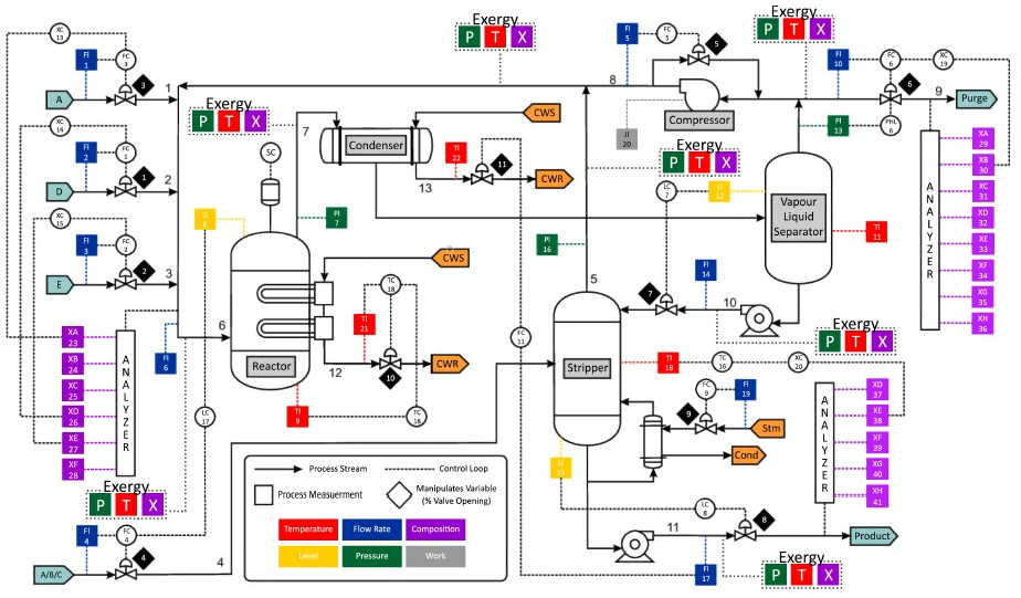
3.2.1. Overview of TE Benchmark Process

The Tennessee Eastman (TE) benchmark is widely recognized as a fundamental reference in the domain of process monitoring, often serving as a pivotal benchmark for validating novel abnormal event detection strategies [55]. Researchers commonly turn to the TE process to assess the effectiveness of their proposed anomaly detection methodologies. The schematic of the TE benchmark process is depicted in Figure 10, and it offers a diverse range of faulty scenarios, including bias, drift, intermittent, random variations, and valve-related abnormalities. These scenarios, detailed in the TE process data sheet, involve the introduction of faults after sampling time instant 160 in the testing data. For the validation process, a total of 22 process measurements (XMEAS 1 to XMEAS 22) and 12 manipulated variables (XMV 42 to XMV 52) are considered [56]. The proposed PCA–KS fault detection strategy’s effectiveness is put to the test by assessing its performance on specific faulty scenarios, namely IDV(1), IDV(2), IDV(4), IDV(5), IDV(6), IDV(7), IDV(8), IDV(10), IDV(11), IDV(12), IDV(13), and IDV(14). Please note that certain fault scenarios, including IDV(3), IDV(9), and IDV(15), have been excluded from this evaluation due to their consistently low False Discovery Rate (FDR) values [56].

Utilizing the fault-free dataset of the TE process, a reference PCA model is constructed using the 500 sampling instances of training fault-free data. To optimize the model, the Cumulative Percentage Variance (CPV) technique is employed, ultimately retaining 19 Principal Components (PCs) from the developed model. This optimized model is then applied to identify various faults within the TE process. For clarity and in-depth evaluation, this study provides a detailed analysis of the proposed PCA–KS strategy’s performance in two specific faulty scenarios—Anomalies IDV(5) and IDV(11) of the TE process. This focused assessment allows us to thoroughly examine the strategy’s effectiveness in detecting anomalies in this complex industrial process.

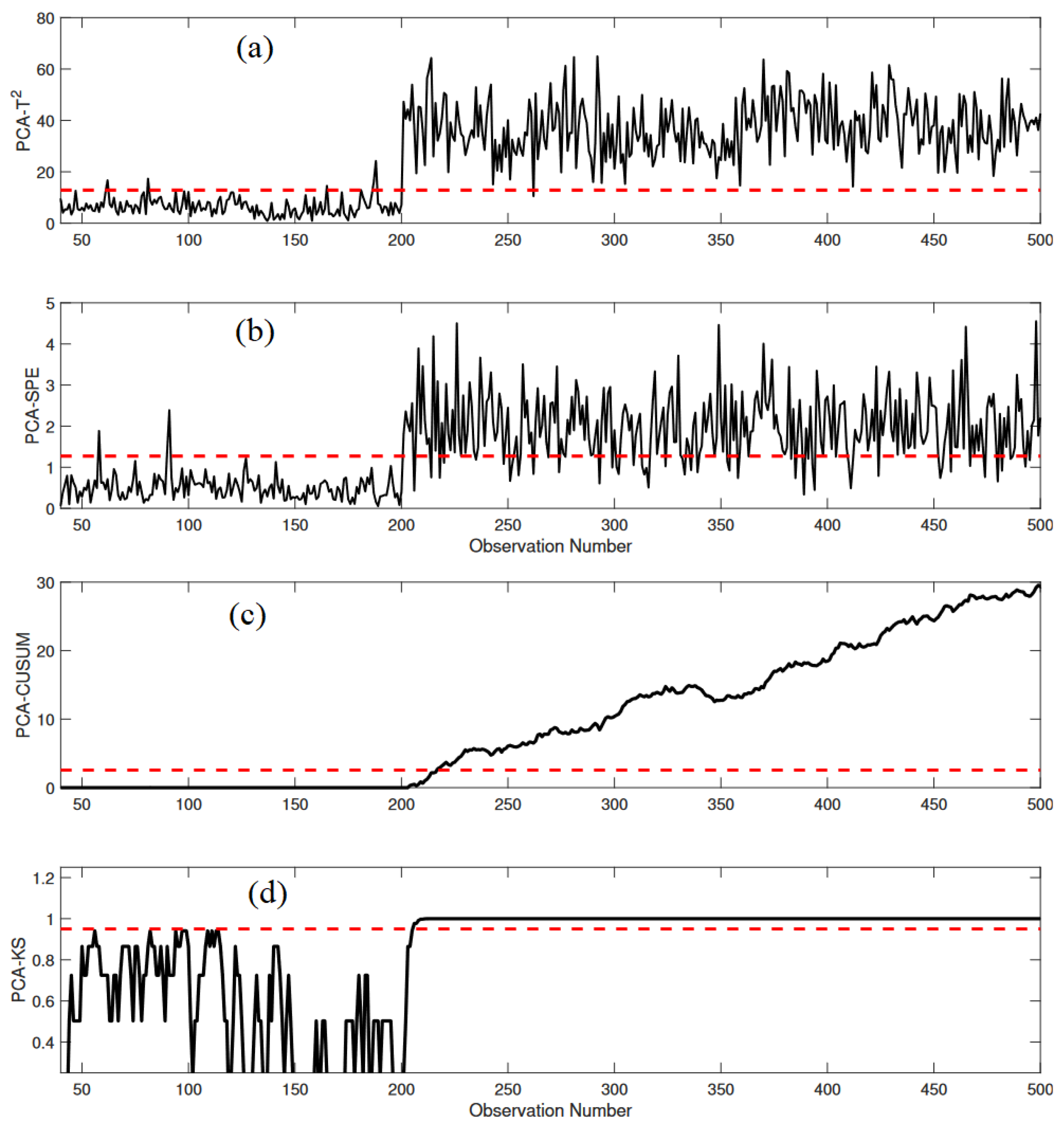
3.2.2. Monitoring Results

For a visual illustration, the performance of the considered fault detection methods in two fault scenarios, namely IDV(5) and IDV(11), will be presented. The IDV(5) fault simulates a step fault in the Condenser cooling water inlet temperature of the TE process. Figure 11a–d displays the monitoring results of the investigated PCA-$T^2$, PCA-SPE, PCA-CUSUM, and PCA–KS-based strategies, respectively. It is noteworthy that both the PCA-$T^2$ and PCA-SPE schemes detect the step fault only within the time frame of sampling instants 160 to 360, with no detection capability beyond sampling instant 360. On the other hand, the PCA-CUSUM scheme outperforms the conventional indicators as it detects this fault within the sampling instants 160 to 460. This extended coverage indicates its improved sensitivity to abnormalities and a better ability to capture the evolving nature of the step fault over time. The proposed PCA–KS strategy stands out with its superior performance. It accurately detects the fault within the defined region, demonstrating the strength of the Kolmogorov–Smirnov test in identifying step faults. By carefully evaluating the statistical properties of the residuals and leveraging the non-parametric approach, PCA–KS excels in detecting anomalies across the entire affected period. This effectiveness is critical in industrial processes where timely detection of faults is essential for preventing costly production losses and ensuring process safety. Therefore, the PCA–KS approach offers a promising solution for accurate and timely fault detection in complex chemical engineering systems such as the TE process.

In the context of the TE process, the IDV(12) scenario simulates random variations in the Reactor cooling water inlet temperature. Monitoring this specific fault is crucial for maintaining process stability and product quality. Figure 12a–d provides a comprehensive view of how different fault detection methods perform in this challenging scenario. The traditional PCA-based fault indicators (i.e., PCA-$T^2$ and PCA-SPE) prove inadequate in precisely detecting this fault. Their performance is compromised, and they are unable to consistently identify the random variations in the Reactor cooling water temperature. Moreover, even the PCA-CUSUM indicators (Figure 12c), which exhibit improved performance in certain fault scenarios, fail to detect this fault effectively, leading to numerous missed detections. These missed detections can be problematic in real industrial settings, potentially causing production disruptions and quality issues. In contrast, the proposed PCA–KS strategy outperforms the traditional indicators. It excels in capturing the subtle and random variations introduced by the IDV(12) fault, resulting in enhanced detection accuracy and minimal missed detections. This capability is vital in industrial applications, where process conditions can change unpredictably, and even minor abnormalities must be identified promptly to avoid operational disruptions.

The performance of different fault detection methods, including PCA-$T^2$, PCA-SPE, PCA-CUSUM, and PCA–KS, in detecting various faults in the TE process is evaluated and summarized in

Table 5. Comparative analysis of the four monitoring methods for detecting five faulty scenarios in the TE process.

Fault	Index	PCA-${\mathit{T}}^2$	PCA-SPE	PCA-CUSUM	PCA–KS
IDV1	FDR	97.95	99.10	94.33	99.65
	FAR	1.63	3.77	0.00	5.00
	Precision	99.10	97.95	100.00	98.02
	Recall	97.95	99.10	94.33	99.65
	F1-score	98.48	98.40	97.08	98.70
IDV2	FDR	94.59	98.52	75.00	98.81
	FAR	1.75	1.75	0.00	9.75
	Precision	99.13	99.16	100.00	95.89
	Recall	94.59	98.52	75.00	98.81
	F1-score	96.67	98.68	85.71	97.77
IDV4	ADR	72.43	97.25	98.00	98.41
	FAR	1.26	1.89	0.00	1.20
	Precision	99.23	99.01	100.00	99.46
	Recall	72.43	97.25	98.00	98.41
	F1-score	83.57	98.25	98.98	98.87
IDV5	ADR	62.16	62.67	93.67	97.94
	FAR	1.18	1.87	0.00	1.50
	Precision	99.12	98.80	100.00	99.25
	Recall	62.16	62.67	93.67	97.94
	F1-score	76.50	76.90	96.71	98.68
IDV6	ADR	98.53	98.63	68.33	99.50
	FAR	0.63	0.78	0.00	7.25
	Precision	99.70	99.71	100.00	97.12
	Recall	98.53	98.63	68.33	99.50
	F1-score	99.22	99.67	81.18	97.93
IDV7	FDR	99.35	99.51	99.51	100.00
	FAR	1.89	3.71	0.00	15.63
	Precision	99.33	98.38	100.00	94.15
	Recall	99.35	99.51	99.51	100.00
	F1-score	99.34	98.90	99.74	97.00
IDV8	FDR	92.43	92.96	92.00	97.94
	FAR	0.63	1.89	0.00	6.88
	Precision	99.76	99.07	100.00	97.09
	Recall	92.43	92.96	92.00	97.94
	F1-score	95.83	95.92	95.83	97.66
IDV10	ADR	33.14	59.82	84.00	95.59
	FAR	1.89	4.50	0.00	10.62
	Precision	97.97	96.85	100.00	95.02
	Recall	33.14	59.82	84.00	95.59
	F1-score	49.57	73.95	90.81	95.61
IDV11	ADR	63.17	73.61	55.00	92.35
	FAR	0.63	5.03	0.00	2.50
	Precision	99.66	92.50	100.00	98.74
	Recall	63.17	73.61	55.00	92.35
	F1-score	77.32	83.67	70.96	95.44
IDV12	ADR	93.67	90.91	79.50	99.51
	FAR	1.89	3.14	0.00	14.37
	Precision	99.17	98.43	100.00	93.59
	Recall	93.67	94.52	79.50	99.01
	F1-score	96.38	86.00	88.57	96.29
IDV13	ADR	87.68	90.62	86.67	89.35
	FAR	0.00	0.00	0.00	0.00
	Precision	100.00	100.00	100.00	100.00
	Recall	87.68	90.62	86.67	89.35
	F1-score	93.43	95.07	93.00	94.24
IDV14	ADR	98.21	94.43	68.50	98.24
	FAR	1.89	1.26	0.00	1.23
	Precision	99.20	99.40	100.00	99.45
	Recall	98.21	94.43	68.50	98.24
	F1-score	98.37	96.85	81.30	98.79

. The results clearly demonstrate the superiority of the proposed PCA–KS approach. It consistently outperforms the other methods, achieving higher F1-scores, which are a key indicator of overall detection performance. The PCA–KS strategy exhibits an advantage in most fault scenarios, reflecting its ability to detect a wide range of abnormalities effectively. These results emphasize the potential of the PCA–KS strategy for enhancing fault detection in the complex and dynamic TE process. Its ability to strike a balance between FDR and FAR while achieving high F1-scores positions it as a valuable tool for improving the reliability and stability of chemical engineering operations.

Table 6. KS test results for TE process fault detection: D-Stat values for fault-free and different fault scenarios in the TE process.

No.	Fault	D-Stat Value
1	No fault	0.2250
2	IDV(1)	0.9894
3	IDV(2)	0.9393
4	IDV(4)	0.9994
5	IDV(5)	0.9825
6	IDV(6)	0.9950
7	IDV(7)	0.8282
8	IDV(8)	0.9195
9	IDV(10)	0.8183
10	IDV(11)	0.8028
11	IDV(12)	0.8995
12	IDV(13)	0.9060
13	IDV(14)	0.9027

provides an overview of the results obtained from the KS test applied to both the fault-free scenario and various faulty scenarios within the TE process. The D-stat values are employed as a key indicator of performance, and their significance is highlighted. The table clearly illustrates the trend, with the D-stat values being lowest for the fault-free scenario, and progressively increasing for each of the different faulty scenarios. This pattern emphasizes the effectiveness of D-stat as a diagnostic tool for identifying anomalies within the TE process. It is important to note that D-stat values near 1 indicate a higher degree of separation between the ECDFs, making them a valuable indicator for distinguishing normal and faulty conditions. This approach helps in effectively characterizing and diagnosing various types of faults in the TE process, thereby contributing to robust anomaly detection strategies.

In summary, the results obtained from the fault detection and monitoring experiments conducted on the PFR and TE processes provide valuable insights into the performance of the proposed PCA–KS method and its comparison with conventional PCA-based indicators such as PCA-$T^2$, PCA-SPE, and PCA-CUSUM. These results collectively underscore the robustness and efficacy of the PCA–KS method for process fault detection in both the PFR and TE processes, along with its ability to consistently outperform conventional PCA-based methods in various fault scenarios. The PCA–KS-based fault detection strategy stands out as a robust and reliable approach, owing to several key advantages. The PCA–KS approach is well-suited to a wide range of data distributions and fault patterns, even when the characteristics of the data are not explicitly known or predictable. Furthermore, the KS statistic is specifically designed to detect differences in the CDFs of two datasets. This inherent capability makes it exceptionally proficient at identifying deviations in data distribution, which often serve as indicators of potential faults. Its sensitivity to distribution changes is a valuable asset when it comes to identifying various types of faults, making it adaptable to diverse industrial scenarios. Moreover, the PCA–KS strategy employs a moving window approach during the computation of the KS statistic. This feature proves to be highly advantageous when working with noisy data or data streams, where the precise location of a fault may not be readily identifiable. The method’s adaptability to changing data patterns over time enhances its applicability in dynamic industrial processes. The KS-based strategy also exhibits a remarkable attribute of maintaining a low false alarm rate while effectively detecting faults. This feature is highly desirable in industrial settings, where erroneous fault alarms can be disruptive and costly. The sensitivity of the KS statistic to even subtle distribution differences enables it to identify small-magnitude faults that might go unnoticed by other methods. This capability is particularly crucial for proactive maintenance and minimizing production disruptions. Finally, the combination of PCA and the KS-based fault detection leverages the strengths of both techniques. PCA streamlines the data by reducing its dimensionality, making it more manageable and interpretable. Meanwhile, the KS statistic zeroes in on the residual errors, enhancing the accuracy of fault detection. This symbiotic relationship between dimensionality reduction and distribution-based anomaly detection underpins the effectiveness of the PCA–KS approach in industrial process monitoring and fault detection.

4. Conclusions

Accurate fault detection is imperative for ensuring the productivity, profitability, and safety of industrial processes. This study introduced an innovative data-based approach that combines the KS indicator with the PCA modeling framework to enhance fault detection in multivariate data. The non-parametric nature of the KS test proved advantageous, as it does not rely on specific assumptions about data distribution, making it versatile across various scenarios. The proposed method effectively identified anomalies in diverse data distributions by computing the distance between normal and online data residuals in a moving window. Significant changes in this distance indicated the presence of faults, with minimal distance in fault-free scenarios and increased distance during faults. Testing the proposed PCA–KS strategy on case studies involving a Plug Flow Reactor (PFR) and the Tennessee Eastman (TE) process demonstrated its robust performance. For the PFR case study, the PCA–KS approach detected various faults with high precision, including bias, intermittent, and sensor-drift faults. It excelled in noisy environments, outperforming conventional methods and achieving high detection performance for the five faulty scenarios in the PFR process. The F1-score values for different faulty scenarios of the PFR process were found to be 100%, 100%, 99.43%, 98.16%, and 97.08%. In the TE process, the PCA–KS strategy precisely detected various faulty scenarios, with F1-scores ranging from 94.24% to 98.87%. The moving window approach employed in the computation of the KS statistic proved advantageous in capturing sensitive details, especially in noisy data or data streams, enhancing the detection of sensor faults. The combination of PCA and the KS statistic offers a powerful solution for industrial process monitoring, reducing data dimensionality while focusing on distribution-based anomaly detection.

5. Future Work: Exploring New Frontiers

Despite the promising performance of the PCA–KS strategy, occasional false alarms were observed in certain Tennessee Eastman process fault scenarios, and while the FAR remains manageable, potential improvements lie ahead. The study concludes by identifying numerous avenues for future research in fault detection in chemical processes. One promising direction is the exploration of adaptive detection thresholds, dynamically adjusting to changing conditions or process variations. The incorporation of an adaptive threshold could enhance the fault detection system’s ability to handle fluctuations effectively, potentially reducing false alarms. Another area of interest involves the integration of a wavelet-based multiscale version of PCA with the KS-based indicator, creating a multi-scale PCA–KS fault detection strategy. This not only accommodates noisy measurements but also improves detection quality by minimizing false alarms. Additionally, investigating the combination of the KS-based monitoring chart with other data-driven methods such as Partial Least Squares (PLS), Canonical Variate Analysis (CVA), or Independent Component Analysis (ICA) presents a valuable avenue for enhancing fault detection capabilities. Furthermore, leveraging the benefits of the KS-based chart in conjunction with deep-learning models, such as long short-term memory and variational autoencoders, could provide robust fault detection for large time-series data. While this study has concentrated on fault detection, future research endeavors should explore fault isolation techniques to pinpoint the root causes of faults in chemical processes. The pursuit of these avenues promises to further advance the field of fault detection and contribute to the reliability and safety of industrial processes.

References

1. Khan, F.I.; Abbasi, S. Major accidents in process industries and an analysis of causes and consequences. J. Loss Prev. Process Ind. 1999, 12, 361–378. [Google Scholar] [CrossRef]
2. Fuente, M.J.D.L.; Sainz-Palmero, G.I.; Galende-Hern¡ndez, M. Dynamic Decentralized Monitoring for Large-Scale Industrial Processes Using Multiblock Canonical Variate Analysis Based Regression. IEEE Access 2023, 11, 26611–26623. [Google Scholar] [CrossRef]
3. Kini, K.R.; Madakyaru, M. Performance Evaluation of Independent Component Analysis-Based Fault Detection Using Measurements Corrupted with Noise. J. Control Autom. Electr. Syst. 2021, 32, 642–655. [Google Scholar] [CrossRef]
4. Shao, L.; Kang, R.; Yi, W.; Zhang, H. An Enhanced Unsupervised Extreme Learning Machine Based Method for the Nonlinear Fault Detection. IEEE Access 2021, 9, 48884–48898. [Google Scholar] [CrossRef]
5. Dhara, V.R.; Dhara, R. The Union Carbide disaster in Bhopal: A review of health effects. Arch. Environ. Health Int. J. 2002, 57, 391–404. [Google Scholar] [CrossRef] [PubMed]
6. Bowonder, B. The bhopal accident. Technol. Forecast. Soc. Chang. 1987, 32, 169–182. [Google Scholar] [CrossRef]
7. Cullen, L.W. The public inquiry into the Piper Alpha disaster. Drill. Contract. 1993, 49. [Google Scholar]
8. Venkatasubramanian, V.; Rengaswamy, R.; Yin, K.; Kavuri, S.N. A review of process fault detection and diagnosis: Part I: Quantitative model-based methods. Comput. Chem. Eng. 2003, 27, 293–311. [Google Scholar] [CrossRef]
9. Lou, Z.; Wang, Y.; Lu, S.; Sun, P. Process Monitoring Using a Novel Robust PCA Scheme. Ind. Eng. Chem. Res. 2021, 60, 4397–4404. [Google Scholar] [CrossRef]
10. Harrou, F.; Sun, Y.; Madakyaru, M.; Bouyedou, B. An improved multivariate chart using partial least squares with continuous ranked probability score. IEEE Sens. J. 2018, 18, 6715–6726. [Google Scholar] [CrossRef]
11. Harrou, F.; Madakyaru, M.; Sun, Y. Improved nonlinear fault detection strategy based on the Hellingerdistance metric: Plug flow reactor monitoring. Energy Build. 2017, 143, 149–161. [Google Scholar] [CrossRef]
12. Alauddin, M.; Khan, F.; Imtiaz, S.; Ahmed, S. A Bibliometric Review and Analysis of Data-Driven Fault Detection and Diagnosis Methods for Process Systems. Ind. Eng. Chem. Res. 2018, 57, 10719–10735. [Google Scholar] [CrossRef]
13. Clark, R.N.; Fosth, D.C.; Walton, V.M. Detecting instrument malfunctions in control systems. IEEE Trans. Aerosp. Electron. Syst. 1975, AES-11, 465–473. [Google Scholar] [CrossRef]
14. Patton, R.J.; Chen, J. A review of parity space approaches to fault diagnosis. IFAC Proc. Vol. 1991, 24, 65–81. [Google Scholar] [CrossRef]
15. Benothman, K.; Maquin, D.; Ragot, J.; Benrejeb, M. Diagnosis of uncertain linear systems: An interval approach. Int. J. Sci. Tech. Autom. Control Comput. Eng. 2007, 1, 136–154. [Google Scholar]
16. Yin, S.; Ding, S.X.; Xie, X.; Luo, H. A review on basic data-driven approaches for industrial process monitoring. IEEE Trans. Ind. Electron. 2014, 61, 6418–6428. [Google Scholar] [CrossRef]
17. Venkatasubramanian, V.; Rengaswamy, R.; Kavuri, S.N.; Yin, K. A review of process fault detection and diagnosis part 3: Process history based methods. Comput. Chem. Eng. 2003, 27, 327–346. [Google Scholar] [CrossRef]
18. Md Nor, N.; Che Hassan, C.R.; Hussain, M.A. A review of data-driven fault detection and diagnosis methods: Applications in chemical process systems. Rev. Chem. Eng. 2020, 36, 513–553. [Google Scholar] [CrossRef]
19. Harrou, F.; Dairi, A.; Sun, Y.; Kadri, F. Detecting abnormal ozone measurements with a deep learning-based strategy. IEEE Sens. J. 2018, 18, 7222–7232. [Google Scholar] [CrossRef]
20. Montgomery, D.C. Introduction to Statistical Quality Control; John Wiley & Sons: Hoboken, NJ, USA, 2019. [Google Scholar]
21. Hawkins, D.M.; Olwell, D.H. Cumulative Sum Charts and Charting for Quality Improvement; Springer Science & Business Media: Berlin/Heidelberg, Germany, 1998. [Google Scholar]
22. Dao, P.B. A CUSUM-Based Approach for Condition Monitoring and Fault Diagnosis of Wind Turbines. Energies 2021, 14, 3236. [Google Scholar] [CrossRef]
23. Lucas, J.M.; Saccucci, M.S. Exponentially weighted moving average control schemes: Properties and enhancements. Technometrics 1990, 32, 1–12. [Google Scholar] [CrossRef]
24. Kresta, J.V.; Macgregor, J.F.; Marlin, T.E. Multivariate statistical monitoring of process operating performance. Can. J. Chem. Eng. 1991, 69, 35–47. [Google Scholar] [CrossRef]
25. Ge, Z.; Song, Z. Multivariate Statistical Process Control: Process Monitoring Methods and Applications; Springer Science & Business Media: Berlin/Heidelberg, Germany, 2012. [Google Scholar]
26. Nawaz, M.; Maulud, A.S.; Zabiri, H.; Suleman, H.; Tufa, L.D. Multiscale Framework for Real-Time Process Monitoring of Nonlinear Chemical Process Systems. Ind. Eng. Chem. Res. 2020, 59, 18595–18606. [Google Scholar] [CrossRef]
27. Li, J.; Yan, X. Process monitoring using principal component analysis and stacked autoencoder for linear and nonlinear coexisting industrial processes. J. Taiwan Inst. Chem. Eng. 2020, 112, 322–329. [Google Scholar] [CrossRef]
28. Sarita, K.; Devarapalli, R.; Kumar, S.; Malik, H.; Garcia Marquez, F.P.; Rai, P. Principal component analysis technique for early fault detection. J. Intell. Fuzzy Syst. 2022, 42, 861–872. [Google Scholar] [CrossRef]
29. Li, W.; Yue, H.H.; Cervantes, S.V.; Qin, S.J. Recursive PCA for adaptive process monitoring. J. Process Control 2000, 10, 471–486. [Google Scholar] [CrossRef]
30. Chai, Y.; Tao, S.; Mao, W.; Zhang, K.; Zhu, Z. Online incipient fault diagnosis based on Kullback Leibler divergence and recursive principle component analysis. Can. J. Chem. Eng. 2018, 96, 426–433. [Google Scholar] [CrossRef]
31. Ku, W.; Storer, R.H.; Georgakis, C. Disturbance Detection and Isolation by Dynamic Principal Component Analysis. Chemom. Intell. Lab. Syst. 1995, 30, 179–196. [Google Scholar] [CrossRef]
32. Bakshi, B.R. Multiscale analysis and modeling using wavelets. J. Chemom. 1999, 13, 415–434. [Google Scholar] [CrossRef]
33. Cheng, T.; Dairi, A.; Harrou, F.; Sun, Y.; Leiknes, T. Monitoring influent conditions of wastewater treatment plants by nonlinear data-based techniques. IEEE Access 2019, 7, 108827–108837. [Google Scholar] [CrossRef]
34. Ahsan, M.; Mashuri, M.; Kuswanto, H.; Prastyo, D.D. Intrusion detection system using multivariate control chart Hotelling’s T2 based on PCA. Int. J. Adv. Sci. Eng. Inf. Technol. 2018, 8, 1905–1911. [Google Scholar] [CrossRef]
35. Nahm, F.S. Nonparametric statistical tests for the continuous data: The basic concept and the practical use. Korean J. Anesthesiol. 2016, 69, 8–14. [Google Scholar] [CrossRef] [PubMed]
36. Harrou, F.; Nounou, M.N.; Nounou, H.N.; Madakyaru, M. Statistical fault detection using PCA-based GLR hypothesis testing. J. Loss Prev. Process Ind. 2013, 26, 129–139. [Google Scholar] [CrossRef]
37. Harmouche, J.; Delpha, C.; Diallo, D. Incipient fault detection and diagnosis based on Kullback-Leibler divergence using principal component analysis: Part II. Signal Process. 2015, 109, 334–344. [Google Scholar] [CrossRef]
38. Zhang, X.; Delpha, C.; Diallo, D. Performance evaluation of Jensen–Shannon divergence-based incipient fault diagnosis: Theoretical proofs and validations. Struct. Health Monit. 2022, 22, 1628–1646. [Google Scholar] [CrossRef]
39. Chen, H.; Jiang, B.; Lu, N. A Newly Robust Fault Detection and Diagnosis Method for High-Speed Trains. IEEE Trans. Intell. Transp. Syst. 2019, 20, 2198–2208. [Google Scholar] [CrossRef]
40. Altukife, F. Nonparametric control chart based on sum of ranks. Pak. J.-Stat. 2003, 19, 291–300. [Google Scholar]
41. Das, N. A non-parametric control chart for controlling variability based on squared rank test. J. Ind. Syst. Eng. 2008, 2, 114–125. [Google Scholar]
42. Diana, G.; Tommasi, C. Cross-validation methods in principal component analysis: A comparison. Stat. Methods Appl. 2002, 11, 71–82. [Google Scholar] [CrossRef]
43. Joe Qin, S. Statistical process monitoring: Basics and beyond. J. Chemom. A J. Chemom. Soc. 2003, 17, 480–502. [Google Scholar] [CrossRef]
44. Harrou, F.; Sun, Y.; Madakyaru, M. Kullback-leibler distance-based enhanced detection of incipient anomalies. J. Loss Prev. Process Ind. 2016, 44, 73–87. [Google Scholar] [CrossRef]
45. Pratt, J.W.; Gibbons, J.D. Kolmogorov-Smirnov Two-Sample Tests. In Concepts of Nonparametric Theory; Springer Series in Statistics; Springer: New York, NY, USA, 1981. [Google Scholar]
46. Guo, P.; Fu, J.; Yang, X. Condition Monitoring and Fault Diagnosis of Wind Turbines Gearbox Bearing Temperature Based on Kolmogorov-Smirnov Test and Convolutional Neural Network Model. Energies 2018, 11, 2248. [Google Scholar] [CrossRef]
47. Test, K.S. The Concise Encyclopedia of Statistics; Springer: New York, NY, USA, 2008. [Google Scholar]
48. Khoshnevisan, D. Empirical Processes, and the Kolmogorov-Smirnov Statistic Math 6070; University of Utah: Salt Lake City, UT, USA, 2006. [Google Scholar]
49. Stephens, M.A. Introduction to Kolmogorov (1933) On the Empirical Determination of a Distribution; Springer: New York, NY, USA, 1992. [Google Scholar]
50. Kar, C.; Mohanty, A. Application of KS test in ball bearing fault diagnosis. J. Sound Vib. 2004, 269, 439–454. [Google Scholar] [CrossRef]
51. Athreya, K.B.; Roy, V. General Glivenko—Cantelli theorems. Stat 2016, 5, 306–311. [Google Scholar] [CrossRef]
52. Singh, R.S. On the Glivenko-Cantelli Theorem for Weighted Empiricals Based on Independent Random Variables. Ann. Probab. 1975, 3, 371–374. [Google Scholar] [CrossRef]
53. Bolbolamiri, N.; Sanai, M.S.; Mirabadi, A. Time-Domain Stator Current Condition Monitoring: Analyzing Point Failures Detection by Kolmogorov-Smirnov (K-S) Test. Int. J. Electr. Comput. Energ. Electron. Commun. Eng. 2012, 6, 587–592. [Google Scholar]
54. Powers, D.M. Evaluation: From precision, recall and F-measure to ROC, informedness, markedness and correlation. arXiv 2020, arXiv:2010.16061. [Google Scholar]
55. Downs, J.; Vogel, E. A plant-wide industrial process control problem. Comput. Chem. Eng. 1993, 17, 245–255. [Google Scholar] [CrossRef]
56. Yin, S.; Ding, S.X.; Haghani, A.; Hao, H.; Zhang, P. A comparison study of basic data-driven fault diagnosis and process monitoring methods on the benchmark Tennessee Eastman process. J. Process Control 2012, 22, 1567–1581. [Google Scholar] [CrossRef]
57. Hu, M.; Hu, X.; Deng, Z.; Tu, B. Fault Diagnosis of Tennessee Eastman Process with XGB-AVSSA-KELM Algorithm. Energies 2022, 15, 3198. [Google Scholar] [CrossRef]
Figure 1. Illustration of (a) similar ECDFs representing consistent data patterns and (b) dissimilar ECDFs depicting divergent data distributions.
Chemengineering 08 00001 g001
Figure 2. Schematic representation of the KS statistic computation between two distributions within a moving window, demonstrating the continuous assessment of differences in data distributions over time.
Chemengineering 08 00001 g002
Figure 3. Block diagram illustrating the key components and workflow of the proposed fault detection strategy.
Chemengineering 08 00001 g003
Figure 4. A schematic diagram illustrating the components and operational aspects of a Plug Flow Reactor, a crucial element in chemical engineering processes.
Chemengineering 08 00001 g004
Figure 5. Detection results of (a) PCA-based T 2 indicator, (b) SPE indicator, (c) CUSUM indicator, and (d) KS indicator in the presence of Fault F2 in the PFR process.
Chemengineering 08 00001 g005
Figure 6. Detection results of (a) PCA-based T 2 indicator, (b) SPE indicator, (c) CUSUM indicator, and (d) KS indicator in the presence of Fault F3 in the PFR process.
Chemengineering 08 00001 g006
Figure 7. Detection results of (a) PCA-based T 2 indicator, (b) SPE indicator, (c) CUSUM indicator, and (d) KS indicator in the presence of Fault F4 in the PFR process.
Chemengineering 08 00001 g007
Figure 8. Detection results of (a) PCA-based T 2 indicator, (b) SPE indicator, (c) CUSUM indicator, and (d) KS indicator in the presence of Fault F5 in the PFR process.
Chemengineering 08 00001 g008
Figure 9. Visual inspection of ECDFs under fault-free and faulty conditions: (a) Empirical CDF of training data residuals (blue line) and testing data residuals (red line) for variable 6 with no fault. (b) Empirical CDF of training data residuals (blue line) and testing data residuals (red line) for variable 6 with fault F2.
Chemengineering 08 00001 g009
Figure 10. A comprehensive schematic representation depicting the key components of the Tennessee Eastman process, a complex and widely studied chemical engineering system [57].
Chemengineering 08 00001 g010
Figure 11. Monitoring results for (a) PCA- T 2 , (b) PCA-SPE, (c) PCA-CUSUM, and (d) PCA–KS in detecting fault IDV(5).
Chemengineering 08 00001 g011
Figure 12. Monitoring results for (a) PCA- T 2 , (b) PCA-SPE, (c) PCA-CUSUM, and (d) PCA–KS in detecting fault IDV(11).
Chemengineering 08 00001 g012