How to Modify LAMMPS: From the Prospective of a Particle Method Researcher

Abstract

LAMMPS is a powerful simulator originally developed for molecular dynamics that, today, also accounts for other particle-based algorithms such as DEM, SPH, or Peridynamics. The versatility of this software is further enhanced by the fact that it is open-source and modifiable by users. This property suits particularly well Discrete Multiphysics and hybrid models that combine multiple particle methods in the same simulation. Modifying LAMMPS can be challenging for researchers with little coding experience. The available material explaining how to modify LAMMPS is either too basic or too advanced for the average researcher. In this work, we provide several examples, with increasing level of complexity, suitable for researchers and practitioners in physics and engineering, who are familiar with coding without been experts. For each feature, step by step instructions for implementing them in LAMMPS are shown to allow researchers to easily follow the procedure and compile a new version of the code. The aim is to fill a gap in the literature with particular reference to the scientific community that uses particle methods for (discrete) multiphysics.

1. Introduction

LAMMPS, acronym for Large-scale Atomic/Molecular Massively Parallel Simulator, was originally written in F77 by Steve Plimpton [1] in 1993 with the goal of having a large-scale parallel classical Molecular Dynamic (MD) code. The project was a Cooperative Research and Development Agreement (CRADA) between two DOE labs (Sandia and LLNL) and three companies (Cray, Bristol Myers Squibb, and Dupont). Since the initial release LAMMPS has been improved and expanded by many researchers who implemented many mesh-free computational methods such as Perydynamics, Smoothed particle hydrodynamics (SPH), Discrete Elemet Method (DEM) and many more [2,3,4,5,6,7,8,9,10,11].

Such a large number of computational methods within the same simulator allows researchers to easily combine them for the simulation of complex phenomena. In particular, our research group has used during the years LAMMPS in a variety of settings that go from classic Molecular Dynamics [12,13,14,15,16], to Discrete Multiphysics simulations of cardiovascular flows [17,18,19,20], Modelling drug adsorption in human organs [21,22,23,24], Cavitation [25,26,27], multiphase flow containing cells or capsules [28,29,30,31], solidification/dissolution [32,33,34], material properties [35,36] and even epidemiology [37] and coupling particles methods with Artificial Intelligence [38,39,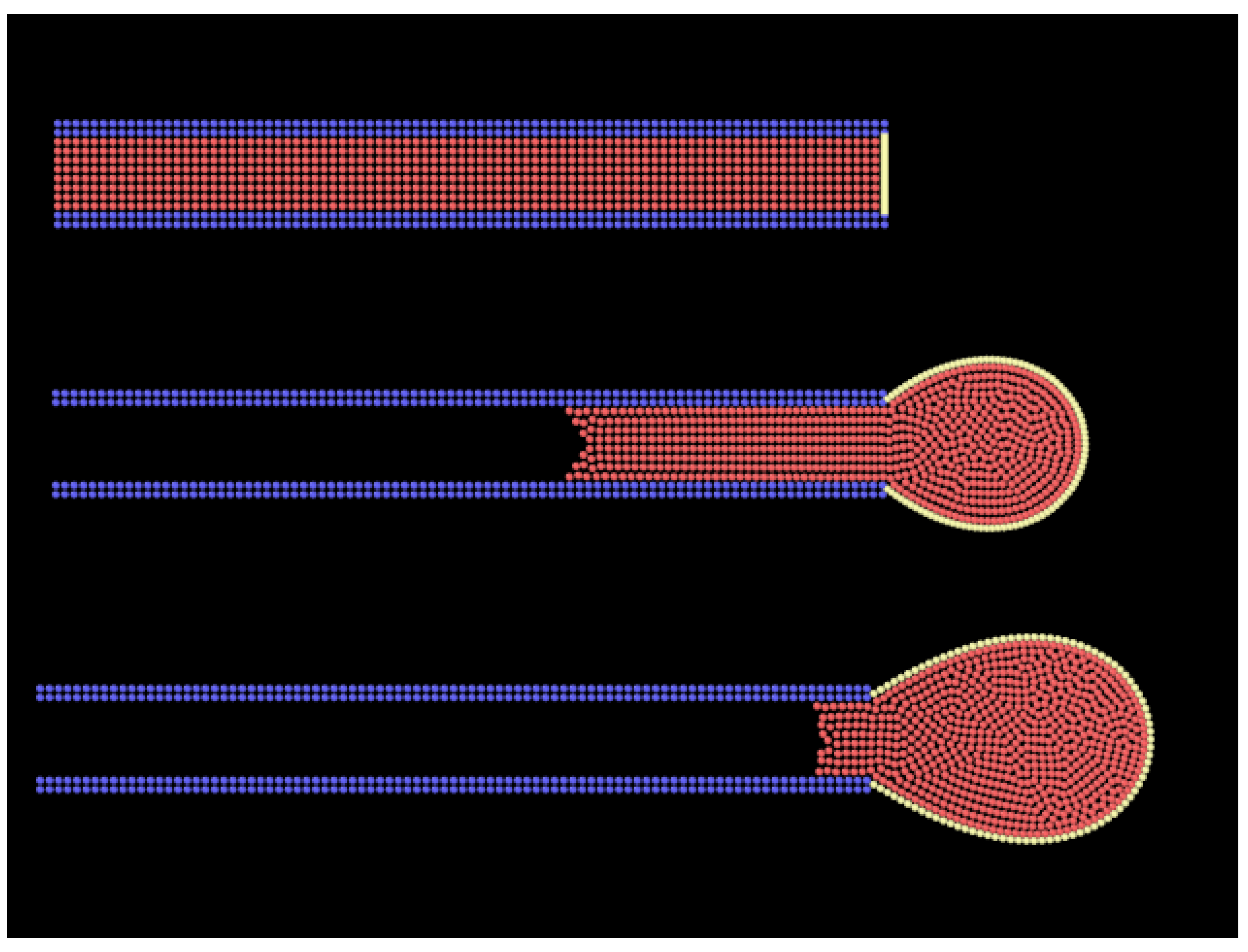40]. An example of a Discrete Multiphysics simulation run with the basic LAMMPS’s code is shown in Appendix A.

Thanks to its modular design open source nature and its large community, LAMMPS has been conceived to be modified and expanded by adding new features. In fact, about 95% of its source code is add-on file [41]. However, this can be a tough challenge for researcher with no to little knowledge of coding. The LAMMPS user manual [41] describes the internal structure and algorithms of the code with the intent of helping researcher to expand LAMMPS. However, due to the lack of examples of implementation and validation, the document can be hard to read for user who are not programmers. In fact, the available material is either very basic [41] or requires advanced programming skills [42,43].

The aim of this work is to provide several step-by-step examples with increasing level of complexity that can fill the gap in the middle to help and encourage researchers to use LAMMPS for discrete multiphysics and expand it with new adds on to the code that could fit their needs. In fact, most of the available material focuses on Molecular Dynamics (MD) and implicitly assumes that the reader’s background is in MD rather than other particle methods such as SPH or DEM. On the contrary, this paper is dedicated to the particle community and highlights how LAMMPS can be used and modified for methods other than MD. This goal fits particularly well with the scope of this Special Issue on “Discrete Multiphysics: Modelling Complex Systems with Particle Methods” In particular, it relates to some of the topics of the Special Issue such by exploring the potential of LAMMPS for coupling particle methods, and by sharing some “tricks of the trade” on how to modify its code that cannot be found anywhere else in the literature.

In Section 2 LAMMPS structure and hierarchy are explained introducing the concept of style. Following the LAMMPS authors advice, to avoid writing a new style from scratch, Section 3, Section 4, Section 5 and Section 6 new styles are developed using existing style are as reference. Finally, in Section 7, all the steps to write a class from scratch are shown.

2. LAMMPS Structure

After initial releases in F77 and F90, LAMMPS is now written in C++, an object oriented language that allows any programmer to exploit the class programming paradigm. The declaration of a class, including the signature of the instance variables and functions (or methods), which can be accessed and used by creating an instance of that class. The data and functions within a class are called members of the class. The definition (or implementation) of a member function can be given inside or outside the class definition.

A class has private, public, and protected sections which contain the corresponding class members.

• The private members, defined before the keyword public, cannot be accessed from outside the class. They can only be accessed by class or “friend” functions, which are declared as having access to class members, without themselves being members. All the class members are private by default.
• The public members can be accessed from outside the class anywhere within the scope of the class object.
• The protected members are similar to private members but they can be accessed by derived classes or child classes while private members cannot.

2.1. Inheritance

An important concepts in object-oriented programming is that of inheritance. Inheritance allows to define a class in terms of another class and the new class inherits the members of the existing class. This existing class is called the base (or parent) class, and the new class is referred to as a subclass, or child class, or derived class.

The idea of inheritance implements the “is a” relationship. For example, Mammal IS-A Animal, Dog IS-A Mammal hence Dog IS-A Animal as well.

The inheritance relationship between the parent and the derived classes is declared in the derived class with the following syntax:

The type of inheritance is specified by the access-specifier, one of public, protected, or private. If the access-specifier is not used, then it is private by default, but public inheritance is commonly used: public members of the base class become public members of the derived class and protected members of the base class become protected members of the derived class. A base class’s private members are never accessible directly from a derived class, but can be accessed through calls to the public and protected members of the base class.

2.2. Virtual Function

The signature of a function f must be declared with a virtual keyword in a base class C to allow its definition (implementation), or redefinition, in a derived class D. Then, when a derived class D object is used as an element of the base class C, and f is called, the derived class’s implementation of the function is executed.

There is nothing wrong with putting the virtual in front of functions inside of the derived classes, but it is not required, unless it is known for sure that the class will not have any children who would need to override the functions of the base class. A class that declares or inherits a virtual function is called a polymorphic class.

2.3. LAMMPS Inheritance and Class Syntax

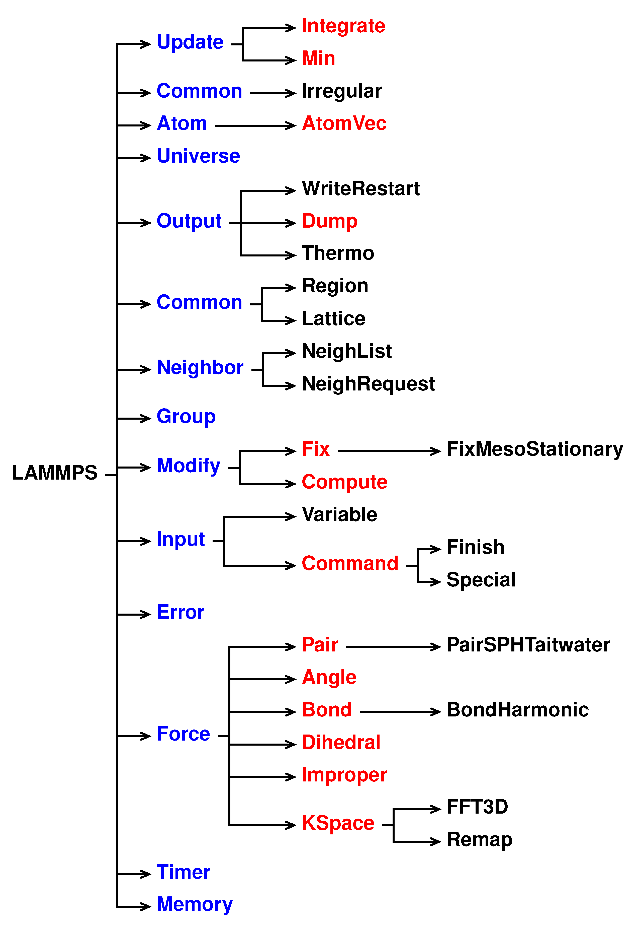
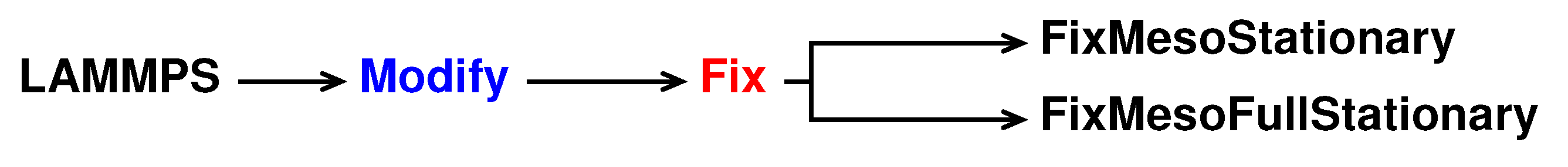
A schematic representation of the LAMMPS inheritance tree is shown in Figure 1: LAMMPS is the top-level class for the entire code, then all the core classes, highlighted in blue, inherit all the constructors, destructors, assignment operator members, friends and private members declared and defined in LAMMPS. The core classes perform LAMMPS fundamental actions. For instance, the Atom class collects and stores all the per-atom, or per-particle, data while Neighbor class builds the neighbor lists [41].

The style classes, highlighted in reds, inherit all the constructors, destructors, assignment operator members, friends and private members declared and defined in LAMMPS and in the corresponding core class. The style classes are also virtual parents class of many child classes that implement the interface defined by the parent class. For example, the fix style has around 100 child classes.

Each style is composed of a pair of files:

• namestyle.h
  The header of the style, where the class style is defined and all the objects, methods and constructors are declared.
• namestyle.cpp
  Where all the objects, methods and constructors declared in the class of style are defined.

When a new style is written both namestyle.h and namestyle.cpp files need to be created.

Each “family” style has its own set of methods, declared in the header and defined in the cpp file, in order to define the scope of the style. For example, the pair style are classes that set the formula(s) LAMMPS uses to compute pairwise interactions while bond style set the formula(s) to compute bond interactions between pairs of atoms [41].

Each pair style has some recurrent functions such as compute, allocate and coeff. Although the final scope of those functions can differ for different styles, they all share a similar role within the classes.

An example of a pair style, sph/taitwater, header in LAMMPS is shown in Listing 2.

All the class members are defined in the cpp file. Taking sph/taitwater pair style as reference, each method declared in Listing 2 will be defined and commented in the next sections. Although this can be style-specific, the aim is to give an overview of how the methods are defined in the cpp in LAMMPS. Albeit different style has different methods, the understanding gained can be transferred into others style, as shown in Section 3 and Section 6.

2.3.1. Constructor

Any class usually include a member function called constructors. The constructor is mechanically invoked when an object of the class is created. This allows the class to initialise members or allocate storage. Unlike the other member of the class, the constructor name must match the name of the class and it does not have a return type.

2.3.2. Destructor

The role of destructors is to de-allocate the allocated dynamic memory, see Section 2.3.8, being mechanically invoked just before the end of the class lifetime. Similarly to constructors, destructors does not have a return type and have the same name as the class name with a tilde ($\sim$) prefix.

2.3.3. compute

compute is virtual member of the pair style and is one of the most relevant functions in a number of classes in LAMMPS. For instance, in pair style classes is used to compute pairwise interaction of the specific pair style. This can seen in the commented Listing 5, where the force applied on a pair of neighboring particles is derived using the Tait equation, lines 131–151. In compute all the local parameters needed to compute the pairwise interaction are declared and defined within the method.

2.3.4. settings

settings is a public void function that reads the input script checking that all the arguments of the pair style are declared. If arguments are present, settings stores them so they can be used by compute. Examples for no arguments pair style and arguments pair style input script with the corresponding settings are listed below:

• No arguments pair style: sph/taitwater
  As described in the SPH for LAMMPS manual [6], the command line to invoke the sph/taitwater pair style is shown in Listing 6.
  In this pair style there is just a string defining the pair style, sph/taitwater, with no arguments. For this reason in settings, Listing 7, when the if statement is true (number of arguments other than zero) an error is produced.
• Arguments pair syle: sph/rhosum
  As described in the SPH for LAMMPS manual [6], the command line to invoke the sph/rhosum pair style is shown in Listing 8.
  In this pair style there is a string defining the pair style, sph/rhosum, plus one argument, Nstep. For this reason in settings, Listing 9, when the if statement is true (number of arguments other than one) an error is produced. When the if statement is false settings assigns the value of Nstep in the variable nstep, line 5, by using the inumeric function defined in the force class.

2.3.5. coeff

Similar to setting, coeff is a public void function that reads and set the coefficients used in by compute of the pair style. For each i j pair is possible to set different coefficients. The coefficients are passed in the input file with the command line pair coeff, see Listing 10. As before, examples for different pair coeff input script and the corresponding coeff are listed below:

• sph/taitwater
  As described in the SPH for LAMMPS manual [6], the command line to invoke sph/taitwater pair coeff is shown in Listing 10.
  In total there are six arguments. Thus, in coeff, Listing 11, when if statement is true (number of arguments other than six) an error is produced. When the if statement is false coeff assigns the type of particles I and J plus the value of rho_0, c_0, alpha and h in from the string to the variables by using the numeric function defined in force class. At last, within the double for loop from line 19 to 32, the variables are assigned for each particles.
• sph/rhosum
  As described in the SPH for LAMMPS manual [6], the syntax to invoke the command is shown in Listing 12.
  In this case there are three arguments. Thus, in the coeff, Listing 13, when the if statement is true (number of arguments other than six) an error is produced. When the error is not produced function assigns the type of particles I and J plus the value of h in the string to the variable cut_one, line 11, by using bounds and numeric function defined in force class. At last, within the double for loop from line 14 to 20, the variables are assigned for each particles.

2.3.6. init_one

init_one check if all the pair coefficients for a given i j pair have been assigned. If they were assigned the methods ensure the symmetry of the matrix.

2.3.7. single

In single the force and energy of a single pairwise interaction, or single bond or angle (in case of bond or angle style), between two atoms is evalutated. The method is specifically invoked by the command line compute pair/local (or compute bond/local) to calculate properties of individual pair, or bond, interactions [41].

2.3.8. allocate

allocate is a protected void function that allocates dynamic memory. The dynamic memory allocation is used when the amount of memory needed depends on user input. As explained before, at the end of the lifetime of the class, the destructors will de-allocate the memory the memory used by allocate.

3. Kelvin–Voigt Bond Style

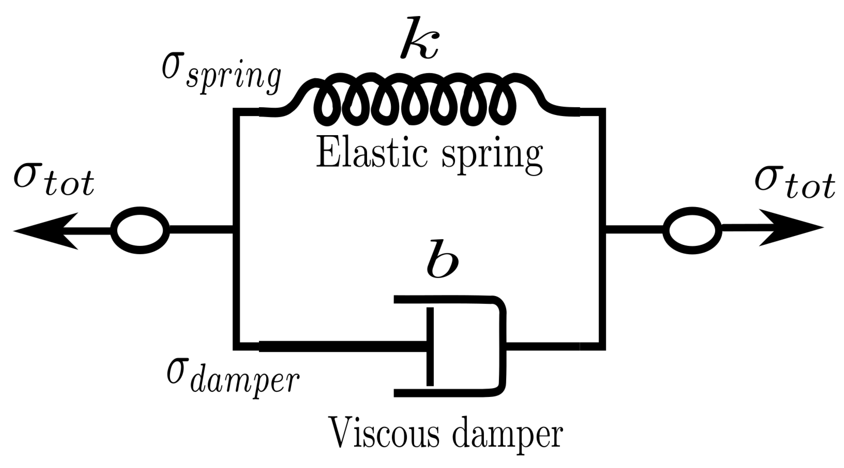
We can use what we learned in the previous section to generate a new dissipative bond potential that can be used to model viscoelastic materials. The Kelvin–Voigt model [44] is used to model viscoelastic material as a purely viscous damper and purely elastic spring connected in parallel as shown in Figure 2.

Since the two components of the model are arranged in parallel, the strain in each component is identical:

$$\begin{array}{c}\hfill {\epsilon }_{tot}={\epsilon }_{spring}={\epsilon }_{damper}.\end{array}$$

(1)

On the other hand, the total stress ${\sigma }_{tot}$ will be split into ${\sigma }_{spring}$ and ${\sigma }_{damper}$ to have ${\epsilon }_{spring}={\epsilon }_{damper}$. Thus we have

$$\begin{array}{c}\hfill {\sigma }_{tot}={\sigma }_{spring}+{\sigma }_{damper}.\end{array}$$

(2)

Combining Equations (1) and (2) with the constitutive relation for both the spring and the dumper, ${\sigma }_{spring}=k\epsilon$ and ${\sigma }_{damper}=b\dot{\epsilon }$, is possible to write that

$$\begin{array}{c}\hfill \sigma =k\epsilon \left(t\right)+b\frac{d\epsilon \left(t\right)}{dt}=k\epsilon \left(t\right)+b\dot{\epsilon },\end{array}$$

(3)

where k is the elastic modulus and b is the coefficient of viscosity. Equation (3) relates stress to strain and strain rate for a Kelvin–Voigt material [44].

Similarly to bond test to write a new pair style called bond kv we take the bond harmonic pair style as reference. The new pair style is declared and initialised in bond_kv.h and bond_kv.cpp saved in the /src/MOLECULE directory and its hierarchy is shown in Figure 3.

3.1. Validation

The bond kv pair style has been validated by Sahputra et al. [45] in their Discrete Multiphysics model for encapsulate particles with a soft outer shell.

3.2. bond_kv.cpp

All the functions will be the same as in the reference bond harmonic. However, in our new bond kv, we need to substitute the “BondHarmonic” text by a new “BondKv” text, as can be seen in Listings 17 and 18. Form now on, when we show a side-by-side comparison between the reference and the modified file, we highlight in yellow the modified lines and in red the deleted lines.

Compared to the bond harmonic we are introducing a new parameter, b, from the input file. For this reason we need to modify destructor, compute, allocate, coeff, write_restart and read_restart. Following the order of function initialisation, see Listing 18, the destructor is modified as shown in Listing 20.

The next function to modify is compute. The strain rate, $\dot{\epsilon }$, can also be seen as the speed of deformation. To use it within the new pair style we need to declared and initialised the velocities of each particles, see Listing 22.

Moreover, inside the loop for (n = 0; n < nbondlist; n++) of the original compute, we need to add a new set of lines between the lines to calculate the spring force and the lines to calculate force and energy increment. Those lines calculate velocities and directions to compute the dashpot forces, see Listing 23.

Now is possible to write the new expression of the force applied to pair of atoms.

With the introduction of a new parameter in the pair style we need to make a new dynamic memory allocation by modifying allocate.

The viscosity of the damper, b, is given by the user in the input file. For this reason, we also need to modify coeff.

This pair style also has the write_restart and read_restart functions that have to be modified. They basically, write and read geometry file that can be used as a support file in the input file.

3.3. bond_kv.h

In the header of the new pair style we need to substitute the “BondHarmonic” text by a new “BondKv” text as well as declare a new protected member in the class, the pointer to b.

3.4. Invoking kv Pair Style

Now the new pair style is completed. To run LAMMPS with the new style we need to compile it and then invoke it by writing the command lines in shown in Listing 34 in the input file.

4. Noble–Abel Stiffened-Gas Pair Style

In the SPH framework is possible to determine all the particles properties by solving the particle form of the continuity equation [6,26]

$$\begin{array}{c}\hfill \frac{d{\rho }_i}{dt}=\sum _j{m}_j{\mathbf{v}}_{ij}{\nabla }_j{W}_{ij};\end{array}$$

(4)

the momentum equation [6,26]

$$\begin{array}{c}\hfill m_i\frac{d{\mathbf{v}}_i}{dt}=\sum _j{m}_i{m}_j\left(\frac{P_i}{{\rho }_i}+\frac{P_i}{{\rho }_i}+{\mathsf{\Pi }}_{ij}\right){\nabla }_j{W}_{ij};\end{array}$$

(5)

and the energy conservation equation [6,26]

$$\begin{array}{c}\hfill m_i\frac{d{e}_i}{dt}=\frac{1}{2}\sum _j{m}_i{m}_j\left(\frac{P_i}{{\rho }_i}+\frac{P_i}{{\rho }_i}+{\mathsf{\Pi }}_{ij}\right):{\mathbf{v}}_{ij}{\nabla }_j{W}_{ij}-\sum _j\frac{m_i{m}_j}{{\rho }_i{\rho }_j}\frac{({\kappa }_i+{\kappa }_j)(T_i-T_j)}{r_{ij}^2}{\mathbf{r}}_{\mathbf{ij}}·{\nabla }_j{W}_{ij}.\end{array}$$

(6)

However, to be able to solve this set of equations an Equation of State (EOS) linking the pressure P and the density $\rho$ is needed [46]. In the user-SPH package of LAMMPS one EOS is used for the liquid (Tait’s EOS) and one for gas phase (ideal gas EOS). In this section we will implement a new EOS for the liquid phase. Note that with similar steps is also possible to implement a new gas EOS.

Le Métayer and Saurel [47] combined the “Noble–Abel” and the “Stiffened-Gas” EOS proposing a new EOS called Noble–Abel Stiffened-Gas (NASG), suitable for multiphase flow. The expression of the EOS does not change with the phase considered. For each phases, the pressure and temperature are calculated as function of density and specific internal energy, e.g.,

$$\begin{array}{c}\hfill P(\rho ,e)=(\gamma -1)\frac{(e-q)}{\left(\frac{1}{\rho }-b\right)}-\gamma P_{\infty },\end{array}$$

(7)

and temperature-wise

$$\begin{array}{c}\hfill T(\rho ,e)=\frac{e-q}{C_v}-\left(\frac{1}{\rho }-b\right)\frac{P_{\infty }}{C_v},\end{array}$$

(8)

where P, $\rho$, e, and q are, respectively, the pressure, the density, the specific internal energy, and the heat bond of the corresponding phase. $\gamma$, $P_{\infty }$, q, and b are constant coefficients that defines the thermodynamic properties of the fluid.

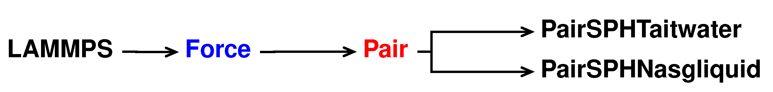
For this new pair style, called sph/nasgliquid, we take as a reference the sph/taitwater pair style declared and initialised in pair_sph_taitwater.h and pair_sph_taitwater.cpp files in the directory /src/USER-SPH. All the files regarding sph/nasgliquid must be saved in the /src/USER-SPH directory and its hierarchy is shown in Figure 4.

4.1. Validation

The sph/nasgliquid pair style has validated by Albano and Alexiadis [26] to study the Rayleigh collapse of an empty cavity.

4.2. pair_sph_nasgliquid.cpp

All the functions will be the same as in the reference sph/taitwater. However, in our new sph/nasgliquid, we need to substitute the “PairSPHTaitwater” text in “PairSPHNasgliquid”, as can be seen in Listings 35 and 36.

For the sph/nasgliquid we need to pass a total of 12 arguments from the input file, while they were only six for sph/taitwater. For this reason we need to modify destructor, compute, allocate, settings and coeff. Following the order of function initialisation, see Listing 36, the destructor is modified as shown in Listing 38.

In the NASG EOS the pressure is function of both density, $\rho$, and internal energy, e. For this reason, we need to declare more pointers and variables in compute compared to the reference pair style, see line 6 and 20 in Listing 40.

Another modification for compute regards the expression of the force applied to the i-th, see Listing 42, and j-th, see Listing 44, particle.

With the introduction of a new parameter in the pair style we need to make a new dynamic memory allocation by modifying allocate.

The 12 arguments used in the pair style are passed by the used in the input file. For this reason, we also have to modify coeff.

4.3. pair_sph_nasgliquid.h

In the header of the new pair style we need to substitute the “PairSPHTaitwater” text in “PairSPHNasgliquid” as well as declare new protected members in the class, the pointers to the new arguments.

4.4. Invoking Sph/Nasgliquid Pair Style

Now the new pair style is completed. To run LAMMPS with the new style we need to compile it and then invoke it by writing the command lines shown in Listing 51 in the input file.

5. Multiphase (Liquid–Gas) Heat Exchange Pair Style

In LAMMPS thermal conductivity between SPH particles is enabled using the sph/heatconduction pair style inside the user-SPH package. However, the pair style is designed only for mono phase fluid where the thermal conductivities is constant (${\kappa }_i=\kappa$). When more than one phase is present, the heat conduction at the interface can be implemented by using [6,26]

$$\begin{array}{c}\hfill m_i\frac{d{e}_i}{dt}=\sum _j\frac{m_i{m}_j}{{\rho }_i{\rho }_j}\frac{({\kappa }_i+{\kappa }_j)(T_i-T_j)}{r_{ij}^2}{\mathbf{r}}_{\mathbf{ij}}·{\nabla }_j{W}_{ij}.\end{array}$$

(9)

In the new pair style, called sph/heatgasliquid, one phase is assumed to be liquid with an initial temperature of $T_{l,0}$ and the other is assumed to be and ideal gas. Each time-step the temperature of the fluid is updated as [26].

$$\begin{array}{c}\hfill T_l=T_{l,0}+\frac{E_l-E_{l,0}}{C_{p,l}},\end{array}$$

(10)

where $T_{l,0}$ is the reference temperature, $E_0$ the internal energy in [J], $E_l$ internal energy [J] at the current time step and $C_{p,l}$ is heat capacity of the fluid in [J K⁻¹]. The temperature of the gas is updated following the ideal EOS [26].

$$\begin{array}{c}\hfill T_g=MM\frac{(\gamma -1)e_g}{R},\end{array}$$

(11)

where $MM$ is the molar mass [kg kmol⁻¹], $e_g$ is the specific internal energy in [J kg⁻¹], $\gamma$ is the heat capacity ratio and R is the ideal gas constant in [J K⁻¹ kmol⁻¹]. Generally the choice of the reference states $E_{l,0}$ is arbitrary, but if the Equation of State (EOS) used for the phase is function of both density and internal energy of the reference state will be determined by the EOS.

In the sph/heatgasliquid pair style is important to check if the i-th and j-th particles are liquid or gas phase to apply either Equation (10) or Equation (11). This “phase check” is explained in Section 5.2 compute function is modified.

For the energy balance the new pair style needs $T_{l,0}$, $E_{l,0}$, $C_{p,l}$ and ${\kappa }_l$ for the liquid phase and ${\kappa }_g$ for the gas phase. Moreover, for the phase check, the particle types of each phases must be specified. All this informations is passed by the user in the in the input file.

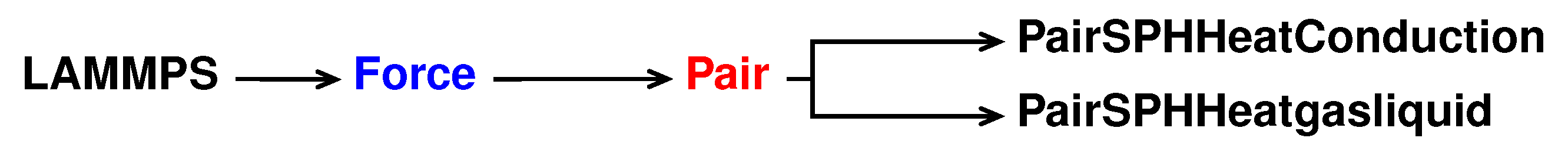
The reference pair style is sph/heatconduction. It is declared and initialised in the pair_sph_heatconduction.cpp pair_sph_heatconduction.cpp files in the directory /src/USER-SPH. All the files regarding sph/heatgasliquid must be saved in the /src/USER-SPH directory and its hierarchy is shown in Figure 5.

5.1. Validation

The sph/heatgasliquid pair style has validated by Albano and Alexiadis [26] to study the role of the heat diffusion in for a gas filled Rayleigh collapse in water.

5.2. pair_sph_heatgasliquid.cpp

All the functions will be the same as in the reference sph/heatconduction. However, in our new sph/heatgasliquid, we need to substitute the “PairSPHHeatConduction” text in “PairSPHHeatgasliquid”, as can be seen in Listings 52 and 53.

For the sph/heatgasliquid we need to pass a total of nine arguments from the input file, while they were only seven for sph/heatconduction. For this reason we need to modify destructor, compute, allocate, settings and coeff. Following the order of function initialisation, see Listing 53, the destructor is modified by removing the heat diffusion coefficient, line 6 in Listing 54.

To compute Equation (6) we need to declare more variables in compute compared to the reference pair style, see line 4 in Listing 57.

Another important modification is to add the phase check inside compute. The phase check has to be implemented for both the i-th particle and the j-th particle inside the loop over neighbours, for (ii = 0; ii < inum; ii++) in the reference pair style. The phase check for the i-th particle starts after the assignment of imass, line 3 of Listing 58.

Similarly, for the j-th the phase check start at line 3 of Listing 59.

The last change in compute is to implement the change in internal energy as shown in Equation (9).

With the introduction of new arguments in the pair style we need to make a new dynamic memory allocation by modifying allocate.

The nine arguments used in the pair style are passed by the user in the input file. For this reason, we also have to modify coeff.

5.3. pair_sph_heatgasliquid.h

In the header of the new pair style we need to substitute the “PairSPHHeatConduction” text in “PairSPHHeatgasliquid” and declare new protected members in the class.

5.4. Invoking Sph/Heatgasliquid Pair Style

Now the new pair style is completed. To run LAMMPS with the new style we need to compile it and then invoke it by writing the command lines shown in Listing 68 in the input file.

6. Full Stationary Fix Style

In LAMMPS a fix style is any operation that is applied to the system, usually to a group of particles, during time stepping or minimisation used to alter some property of the sytem [41]. There are hundreds of fixes defined in LAMMPS and new ones can be added. Usually fixes are used for time integration, force constraints, boundary conditions and diagnostics.

In the user-sph package in LAMMPS there is the so called meso/stationary fix used to set boundary condition. With meso/stationary is possible to fix position and velocity for a group of particles, walls as example, but internal energy and density will be updated. In some cases, it is useful to have a fully stationary conditions that maintains constant also the energy and the density. For this new fix, called meso/fullstationary, we take as a reference the meso/stationary fix declared and initialised in fix_meso_stationary.h and fix_meso_stationary.cpp files in the directory /src/USER-SPH. All the files regarding meso/fullstationary must be saved in the /src/USER-SPH directory and its hierarchy is shown in Figure 6.

6.1. Validation

The meso/fullstationary has been used in the validation of the new viscosity class to set the boundary condition of a constant asymmetric heated walls, see Section 7.2.

6.2. fix_meso_fullstationary.cpp

All the functions will be the same as in the reference meso/stationary. However, in our new fullstationary, we need to substitute the “FixMesoStationary” text in “FixMesoFullStationary”, as can be seen in Listings 69 and 70.

For the meso/fullstationary we need to modify two function: initial_integrate, see Listing 72 line 16 and 17, and final_integrate, see Listing 74 line 14 and 15.

6.3. fix_mes_fullstationary.h

In the header of the new fix we need to substitute the “FixMesoStationary” text in “FixMesoFullStationary”.

6.4. Invoking Meso/Fullstationary Fix

Now the new fix is completed. To run LAMMPS with the new style we need to compile it and then invoke it by writing the command lines shown in Listing 77 in the input file.

7. Viscosity Class

Viscosity in the SPH method has been addressed with different solutions [46]. Shock waves, for example, have been a challenge to model due to the arise of numerical oscillations around the shocked region. Monaghan solved this problem with the introduction of the so-called Monaghan artificial viscosity [48]. Artificial viscosity is still used nowadays for energy dissipation and to prevent unphysical penetration for particles approaching each other [25,49]. The SPH package of LAMMPS uses the following artificial viscosity expression [6], within the sph/idealgas and sph/taitwater pair style.

$${\mathsf{\Pi }}_{ij}=-\alpha h\frac{c_i+c_j}{{\rho }_i+{\rho }_j}\frac{{\mathbf{v}}_{ij}·{\mathbf{r}}_{ij}}{r_{ij}^2+ϵh^2},$$

(12)

where $\alpha$ is the dimensionless dissipation factor, $c_i$ and $c_j$ are the speed of sound of particle i and j. The dissipation factor, $\alpha$, can be linked with the real viscosity in term of [6]

$$\alpha =8\frac{\mu }{ch\rho },$$

(13)

where c is the speed of sound, $\rho$ the density, $\mu$ the dynamic viscosity and h the smoothing length.

The artificial viscosity approach performs well at a high Reynolds number but better solutions are available for laminar flow: Morris et al. [50] approximated and implemented the viscosity momentum term for SPH. The same solution can be found in the sph/taitwater/morris pair style with the expression [6].

$$\sum _j\frac{m_i{m}_j({\mu }_i+{\mu }_j){\mathbf{v}}_{ij}}{{\rho }_i{\rho }_j}\left(\frac{1}{r_{ij}}\frac{\partial W_{ij}}{\partial r_i}\right),$$

(14)

where $\mu$ is the real dynamic viscosity.

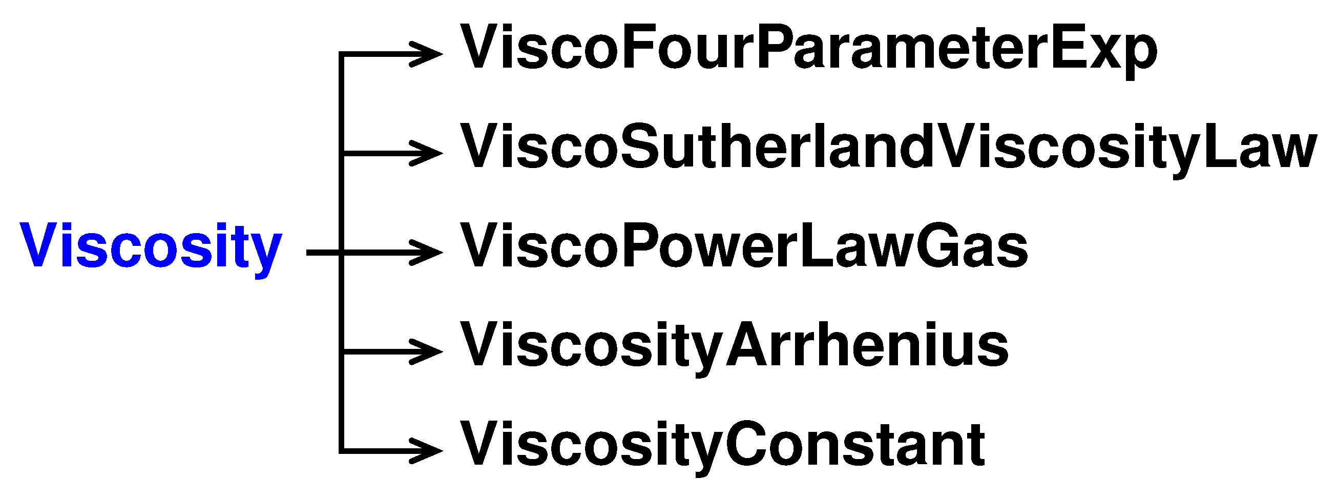
In LAMMPS both the dissipation factor and the dynamic viscosity are treated as a constant between a pair of particles when they interact within the smoothing length. In this section we want to make the viscosity a per atom property instead of a pair property only existing within a pair style. Moreover, five temperature dependent viscosity models are added. For this example, no reference file is used; a new class, Viscosity, is implemented in LAMMPS from scratch and its hierarchy is shown in Figure 7.

7.1. Temperature Dependant Viscosity

In literature multiples empirical models that correlate viscosity with temperature are available [51,52,53]. In the new viscosity class five different viscosity models have been implemented:

1.

Andrade’s equation [54]

$$\mu =Aexp\left(\frac{B}{T}+CT+D{T}^2\right),$$

(15)

where $\mu$ is the viscosity in [Kg m⁻¹ s⁻¹], T is the static temperature in Kelvin, A, B, C and D are fluid-dependent dimensional coefficients available in literature.

2.

Arrhenius viscosity by Raman [55,56]

$$\mu =C_{1}exp\left(C_2/T\right),$$

(16)

where $\mu$ is the dynamic viscosity in [Kg m⁻¹ s⁻¹], T is the temperature in Kelvin, $C_1$ and $C_2$ are fluid-dependent dimensional coefficients available in literature.

3.

Sutherland’s viscosity [57,58] for gas phase

Sutherland’s law can be expressed as:

$$\mu =\frac{C_1{T}^{3/2}}{T+C_2},$$

(17)

where $\mu$ is the viscosity in [Kg m⁻¹ s⁻¹], T is the static temperature in Kelvin, $C_1$ and $C_2$ are dimensional coefficients.

4.

Power-Law viscosity law [57] for gas phase

A power-law viscosity law with two coefficients has the form:

$$\mu =B{T}^n,$$

(18)

where $\mu$ is the viscosity in [Kg m⁻¹ s⁻¹], T is the static temperature in Kelvin, and B is a dimensional coefficient.

5.

Constant viscosity

With constant viscosity both dissipation factor and dynamic viscosity will be constant during the simulation.

When the artificial viscosity is used the dissipation factor of Equation (12) is defined as the arithmetic mean of the dissipation factors of i-th particle and j-th particle.

$${\alpha }_{ij}=-\frac{4}{h}\left(\frac{{\mu }_i}{c_i{\rho }_i}+\frac{{\mu }_j}{c_j{\rho }_j}\right),$$

(19)

where ${\alpha }_{ij}$ is the dissipation factor of the particles pair i and j.

7.2. Validation

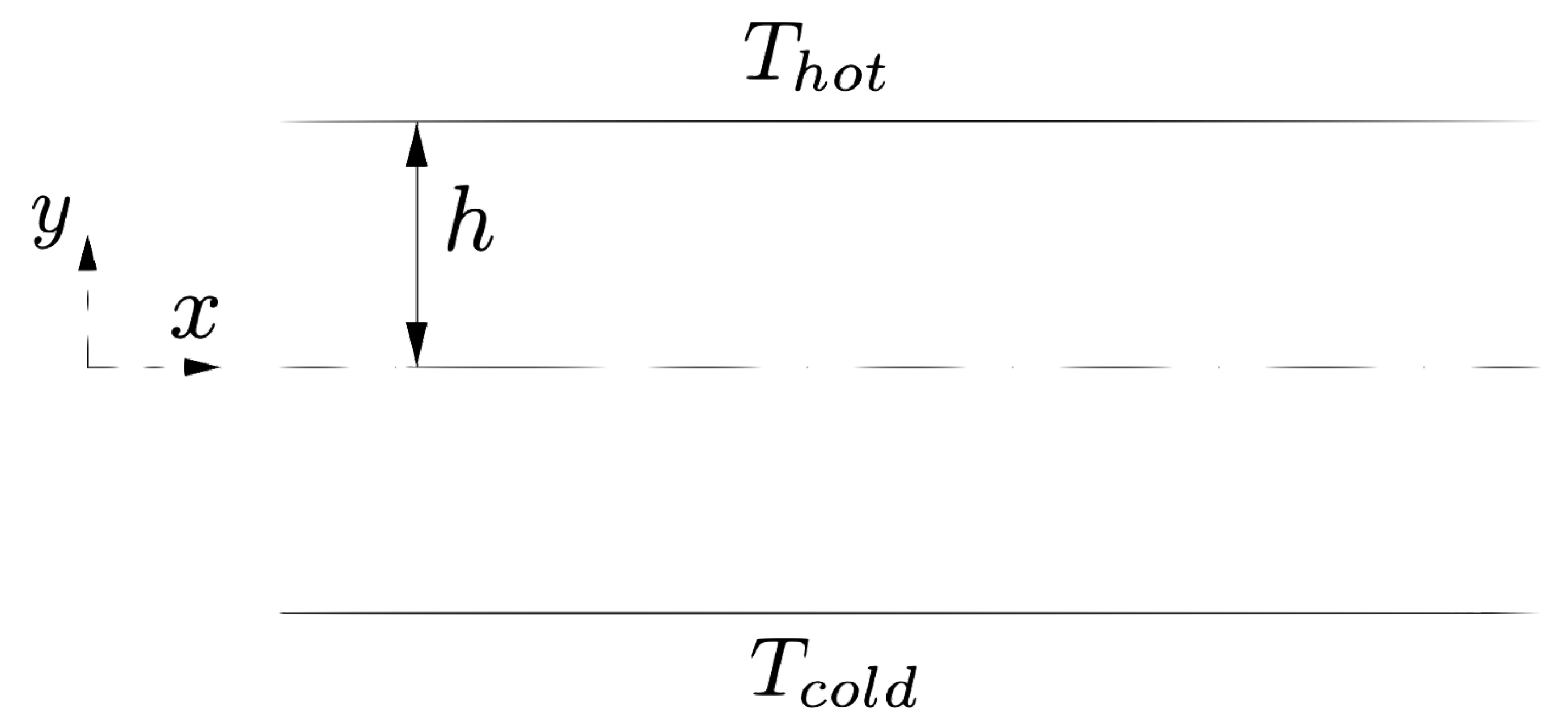
In order to validate the new Viscosity class, we will study the effect of asymmetrically heating walls in a channel flow, and more specifically the effect on the velocity field of the fluid. The data obtained with our model will be compared with the analytical solution obtained by Sameen and Govindarajan [59].

The water flows between two walls in the x-direction with periodic conditions. The walls are set at different temperatures $T_{cold}$ and $T_{hot}$, see Figure 8. Both water and walls are modelled as fluid following the tait EOS. The physical properties of the walls are set constant throughout the simulation using the full stationary conditions described in Section 6.

To match the condition used by Sameen and Govindarajan we set the cold wall temperature to $T_{cold}=295$ K and the temperature dependence of the dynamic viscosity described by the Arrhenius model, Equation (16), with $C_1=0.000183$ [Ns m⁻²] and $C_2=1879.9$ K [59]. To describe the asymmetric heating Sameen and Govindarajan introduced the parameter m, defined as:

$$m=\frac{{\mu }_{cold}}{{\mu }_{ref}}$$

(20)

where ${\mu }_{ref}={\mu }_{hot}$ is the viscosity at the hot wall in the case of asymmetric heating and ${\mu }_{cold}$ is the viscosity at the cold wall. By combining (16) and (20), with the given $T_{cold}$, is possible to express the temperature difference of the walls $\Delta T$ as function of m.

Figure 9 shows the viscosity trend for different values of m and the corresponding $\Delta T$. Sometimes, in particle methods, instantaneous data can be noisy (scattered) as can be seen from the blue circles of both Figure 9 and Figure 10.

In all the cases considered, the model is in good agreement with the work of Sameen and Govindarajan.

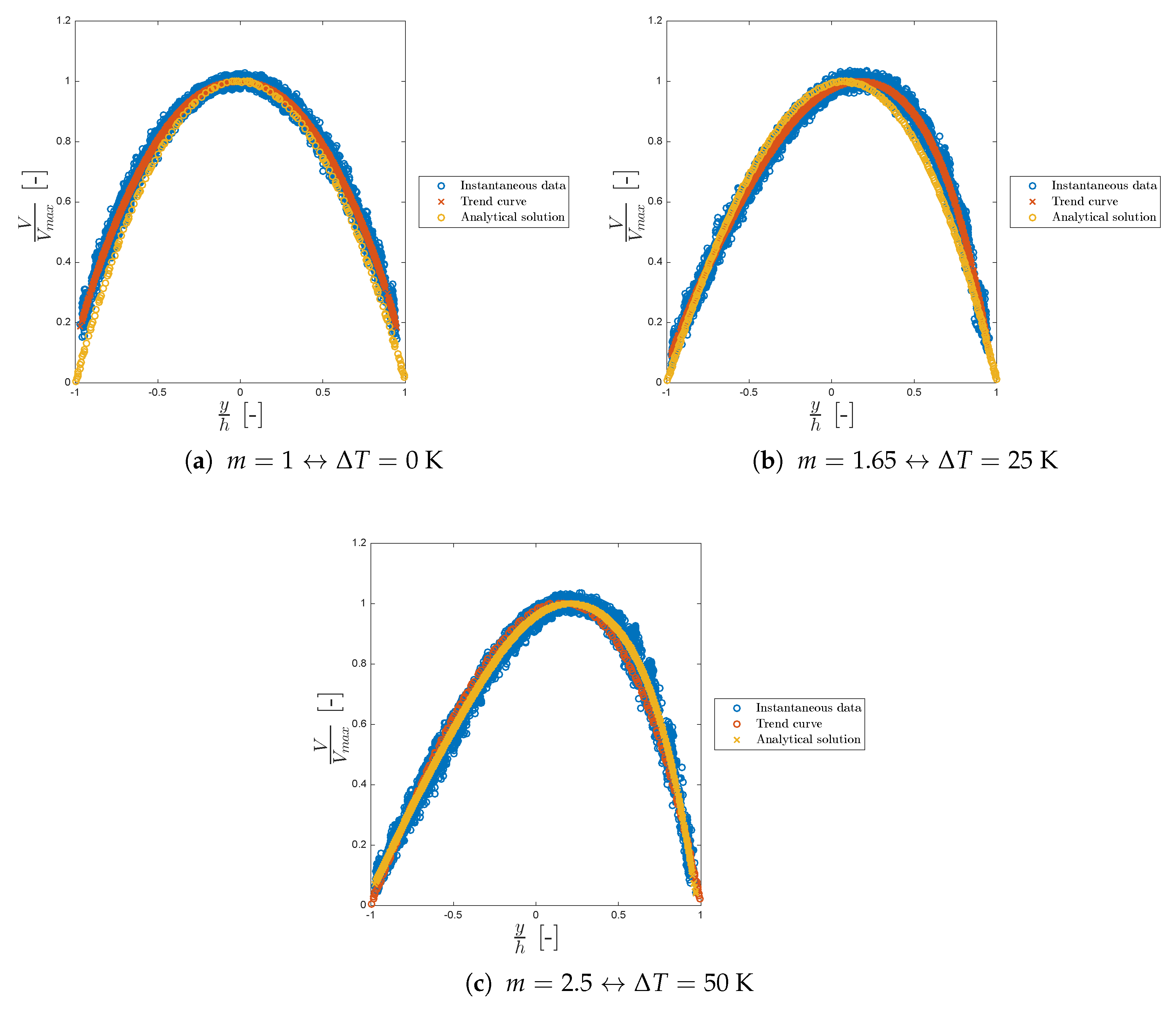
Figure 10 shows the dimensionless velocity trend for different values of m.

Again, the model is in good agreement with the analytical solution of Sameen and Govindarajan always laying within the velocity scattered points. In both our model and in the analytical solution the maximum of the velocity shifts to the right as m increases. We can conclude that our model is in good agreement with the literature, showing the typical viscosity and velocity profiles for asymmetric heating confirming the correct functionality of the new viscosity class.

7.3. New Abstract Class: Viscosity

To implement the new viscosity model a new abstract class has been created, called Viscosity. The class has no attribute, and one virtual method: compute_visc, that is used to compute the viscosity using one of the Equations (15)–(18). As usual, the Viscosity class is divided in two files, see Listings 78 and 79. As it is an abstract class, it cannot be instantiated. It is used as a base, a mold, to implement the viscosity models. All implemented viscosity classes, such as the ones implementing the Arrhenius viscosity or the Sutherland viscosity, will inherit from this class.

This type of base class is called an interface, though as the code is written in C++, there is no actual difference in the implementation. The difference is only in concepts.

This structure allows for a very simple procedure to add a new viscosity type to LAMMPS, as one doesn’t have to go through all of the code everytime a new viscosity type is implemented. All that is required is to implement a new viscosity class inheriting from the Viscosity abstract class and modify the add_viscosity function. The details of the changes required for those two actions are detailed later in this section.

Another structure one might think of to implement the viscosity abstract base class would be a template. Indeed, templates are more efficient than inherited classes as inherited classes create additional virtual calls when calling the class’s methods. However, the choice of which viscosity should be called is made at runtime, and not at compile time, which means the abstract base class would be a better fit. When runtime polymorphism is needed, the structure preferred is an abstract base class.

The abstract class is not the most efficient implementation, but it allows for simplicity of use, which is important considering most of LAMMPS users are not programmers. In this work, we have chosen to sacrifice a bit of efficiency to gain ease of use.

7.4. Implementing a New Viscosity Class

In this section the steps to implement one of Equations (15)–(18) are shown, using the four parameter exponential viscosity as an example.

A new class is created that inherits from the Viscosity abstract class. The new class have as much attributes as the viscosity type has parameters. In this example that means four, as shown in the header in Listing 80.

The constructor therefore should take as arguments the four parameters of the Andrade’s equation and initialise the class’s attributes with those values. The last step is to implement the compute_visc method so it returns the value of the viscosity at the given temperature. The implementation of both those functions is shown in Listing 81.

Similar steps have to be taken to implement the classes corresponding to the other viscosity models, see the Supplementary material.

7.5. Processing the Viscosity in the Atom Class

In the header of the Atom class we need to include the new viscosity class and declare a new set of public members.

We add two new attributes in the USER-SPH section of the Atom attribute lists: viscosity, a pointer to a Viscosity object and viscosities, a pointer to an array containing the values of dynamic viscosities for all atoms at the current time step.

We want to be able to choose which type of viscosity is being used in the simulation from the input file, using a new command called viscosity. Let’s discuss the implementation of this feature. First we need to define the viscosity command. This is done by modifying the execute_command method of the Input class. We then define a new function called add_viscosity, whose declaration is shown in Listing 86 and definition in Listing 87. This function will have to be modified each time one wants to create a new viscosity class. In add_viscosity, the element arg[0] is the string representing the type of viscosity. For each viscosity class, the method performs the following procedure:

• It checks which type of viscosity is asked to be created using the function strcmp on arg[0] (for Andrade’s viscosity it corresponds to line 3 of Listing 87)
• It checks if the number of arguments is coherent with the number of parameter of the viscosity type (line 4–5)
• It scans the coefficients of that viscosity type (line 6–10)
• It creates the appropriate viscosity and initializes the Viscosity attribute (line 11).

This process should be followed for any new implementation.

All headers of the new viscosity types implemented in the add_viscosity function need to be included in the Atom class, see Listing 88.

The viscosity attribute is initialised to NULL in the constructor, see Listing 89.

In the destructor of the Atom class, we add a line to delete the viscosity attribute, see Listing 90.

The extract function is modified to process the viscosity attribute, see Listing 91.

7.6. Using compute_Visc in SPH Pair Styles: Tait Water Implementation

The dynamic viscosity is used to compute the artificial viscosity force, that is used in the compute function of the following SPH pair style: sph/idealgas, sph/lj, sph/taitwater and sph/taitwater/morris. In this section the steps to implement compute_visc in sph/taitwater are shown, the others required a similar procedure.

The first function to modify is the destructor, as we don’t have to allocate the viscosity parameter anymore.

For the same reason as the destructor we need to modify allocate.

Inside the compute function of the sph/taitwater pair style we need to declare a new set of variables. Where e is the energy and $cv$ the heat capacity, now needed to calculate the temperature and thus the viscosity.

The next modification is inside the loop over the j-th atom when the force induced by the artificial viscosity is calculated inside the pair’s compute function.

The dynamic viscosities ${\mu }_i$ and ${\mu }_j$ are calculated for each atoms, using the formula implemented in the compute_visc method. The temperature for the i-th atom is obtained using $T_i=e_i/c{v}_i$. It is important to note that using such expression for the energy balance prevents the reference state of the internal energy to be set at 0.

The constant viscosity matrix element is replaced by the formula defined in Equation (19), see Listings 97 and 98.

Viscosity is now a per atom property, this means that we don’t have to pass its value then the pair style is invoked. For this reason we need to delete the viscosity related lines inside coeff.

The last modification is in init_one. Again, we delete lines related to the former viscosity attribute.

7.7. Running the New Software with Mpirun

At this stage, the software is designed to only run in serial. Changes need to be made to make it run with Message Passing Interface (MPI). This will allow the software to run in parallel: some computations being independent from each other, they can be performed at the same time. Instead of using one processor for a long time, we will use multiple processors for a shorter period. The simulation will therefore take more computing resources but will take a lot shorter to compute. The original SPH module can already be run with MPI however as we have modified the code that is no longer true. We need to make additional changes to the software. All those changes are located in the Atom Vec Meso class of the SPH module.

In LAMMPS, the different MPI processes have to communicate with each other as the computations they perform are not completely independent from each other. They need data from other processes in order to perform their own calculations. They communicate with each other using a buffer that will contain all the necessary data. The buffer is simply an array that we will fill with the data. The different methods for packing and unpacking this buffer are defined in the Atom Vec Meso class. We need to add a new data to transmit: the calculated viscosity.

The first thing to do is to increase the size of the buffers in their initialisation so they can accept the viscosity value, an example is shown in Listings 103 and 104.

Then, we added the relevant elements of the attribute viscosities to the buffer in all the methods handling buffers, an example is shown in Listings 105 and 106.

After making those changes for all the methods in the class, the software can be run using mpirun.

7.8. Invoking, Selecting and Computing a Viscosity Object

To compute the new viscosity a new argument was added to the compute command: viscosities. This allows the user to use the compute command to output the dynamic viscosity to the dump file. This can be done by the following command:

The implementation of this feature is simple, as it is very similar to other compute argument implementation. All that needs to be done is to modify another compute’s implementation, such as compute_meso_rho_atom so it processes the variable viscosities instead of rho.

The viscosity used in the simulation can be invoked in the input file, using the following command:

The type of viscosity can be chosen from the following list:

• FourParameterExp: the four parameter exponential viscosity law.
• SutherlandViscosityLaw: the Sutherland viscosity law.
• PowerLawGas: the power viscosity law for gases.
• Arrhenius: the Arrhenius viscosity law.
• Constant: a constant viscosity.

For example, to invoke the four parameter exponential viscosity, we can write in the input file:

As stated earlier, this list can easily be extended by the user by modifying the add_viscosity function defined earlier.

8. Conclusions

Particle methods are very versatile and can be applied in a variety of applications, ranging from modelling of molecules to the simulation of galaxies. Their power is even amplified when they are coupled together within a discrete multiphysics framework. This versatility matches well with LAMMPS, which is a particle simulator, whose open-source code can be extended with new functionalities. However, modifying LAMMPS can be challenging for researchers with little coding experience and the available support material on how to modify LAMMPS is either too basic or too advanced for the average researcher. Moreover, most of the available material focuses on MD; while the aim of this paper is to support researchers that use other particle methods such as SPH or DEM.

In this work, we present several examples, explained step-by-step and with increasing level of complexity. We begin with simple cases and concluding with more complex ones: Section 3 shows the implementation of the Kelvin–Voigt bond style used to model encapsulate particles with a soft outer shell and validated validated by simulating spherical homogeneous linear elastic and viscoelastic particles [45]; Section 7 show how to implement a new per-atom temperature dependant viscosity property and is validated finding the same viscosity and velocity trend shown by Sameen and Govindarajan [59] in their analytical solution for a channel flow in a asymmetrical heating walls.

The work perfectly fits in the “Discrete Multiphysics: Modelling Complex Systems with Particle Methods” special issue by sharing some in dept know-how and “trick and trades” developed by our group in years of use of LAMMPS. In fact, the aim is to support, in several ways, researchers that use computational particle methods. Often researchers tend to write their own code. The advantage of this approach is that the code is well understood by the researcher and, therefore, easily extendible. However, this sometimes implies reinventing the wheel and countless hours of debugging. Familiarity with a code like LAMMPS, which has an active community of practice and is periodically enriched with new features would be beneficial to this type of researchers allowing them to save considerable time. In the long term, there is another advantage. Modules written for in-house code are hardly sharable. At the moment, the largest portion of the LAMMPS community is dedicated to MD. While this article was under review, for instance, a new book dedicated to modifying LAMMPS came out [60]. However, it focuses only on MD and it does not mention other discrete methods like SPH or DEM. Instead, the aim of this paper is to make LAMMPS more accessible for the Discrete Multiphysics community facilitating sharing reusable code among practitioners in this field.