Experimental Methods for Measuring the Breakup Frequency in Turbulent Emulsification: A Critical Review

Abstract

The growing interest in using population balance modeling to describe emulsification processes has spurred an interest in experimentally measuring the breakup frequency. This contribution classifies, compares, and critically reviews the different methods that have been suggested for measuring the breakup frequency, applicable to emulsification devices. Two major approaches can be seen in previous studies. The first is ‘single drop breakup experiment’-based studies, which estimate the breakup frequency by observing the fate of individual drops. The second approach involves ‘emulsification experiment’-based studies, which combine measured drop-size distributions with assumptions to allow for estimations of the breakup frequency. This second approach can be further subdivided in three types: Parametric determination, inverse self-similarity-based methods, and direct back-calculation methods. Each of these methods are reviewed in terms of their implementation, reliability, and validity. Suggestions of methodological considerations for future studies are given for each class, together with more general suggestions for further investigations. The overall objective is to provide emulsification researchers with background information when choosing which method to use for measuring the breakup frequency and with support when setting up experiments and data evaluation procedures.

1. Introduction

Emulsification—the dispersion of two immiscible fluids, one in the other—is an important unit operation in many food, pharmaceutical, and general chemical engineering processes (e.g., in the production of homogenized dairy products, sauces, and dressings, as well as in the production of infusion fluids and creams for topical drug delivery). Two different types of emulsification processes can be distinguished [1,2]: The ‘low energy methods’, such as membrane emulsification and inverse phase inversion methods, and the ‘high energy methods’, such as rotor-stator emulsification and high-pressure homogenization. This latter class of processes is the most commonly found in industry today, mainly because it allows for continuous production on a large scale.

From a fluid dynamic perspective, many of the high energy emulsification techniques are similar. For example, both rotor-stator mixers and high-pressure homogenizers rely on forcing the pre-emulsion through a narrow gap at high velocities, giving rise to an intense turbulent jet [3,4,5]. Single drop breakup visualizations in both devices show that drop deformation and subsequent breakup take place in this turbulent jet created after the gap [6,7,8]. Experiments on other devices used for emulsification show, at least qualitatively, similar results, e.g., for turbulent dispersion following pipe constriction [9,10], for emulsification in turbulent jets [11,12], and for emulsification in a stirred turbulent batch tank [13,14].

This turbulent drop breakup is relatively well-understood in terms of how the resulting average drop diameter scales with operating conditions and underlying properties of the turbulence [1,15,16,17,18]. However, during the last few decades, there has been a growing interest in trying to understand the dynamics of the breakup process. More specifically, there has been an increasing interest in describing and ultimately predicting how the drop size distribution (DSD) changes dynamically when subjected to a turbulent flow field, especially in industrial emulsification devices [19]. The ultimate objective of these investigations is to predict how the emulsion characteristics vary with the mechanical design of the emulsification device, the physical properties of the fluids, and the operating conditions, thus allowing for both an increased fundamental understanding and a model-based design workflow for optimizing the design and operation.

The population balance equation (PBE)—a mass balance describing the redistribution of drop volume between size classes due to, for example, breakup [20,21]—is the modeling framework predominantly used for predicting the evolution of the DSD in turbulent emulsification. Several studies attempting to predict the evolution of the DSD due to turbulent emulsification have been published [22,23,24,25].

However, the PBE framework must be combined with mathematical models (‘kernels’) describing fragmentation (and coalescence, if present), in order to give any predictions. For a purely fragmenting system, two kernels are needed: The breakup frequency (defined as the number of drops breaking per unit time) and the fragment size distribution (defined as the number of fragments formed of a certain volume from breaking a drop with a given volume). A large number of breakup frequency models have been suggested, and are reviewed elsewhere [26,27,28]. Moreover, new suggestions are continuously being proposed [29]. However, there is of yet no wide consensus on which breakup frequency model is most suitable, not even for the most idealized case of homogenous and isotropic turbulence. Since the turbulence inside an emulsification device is typically severely non-ideal [30], it is not possible to choose which fragmentation kernels to use in a PBE from theory alone. This confusion in terms of how to model the breakup frequency is a clear limitation in all attempts to use PBEs for turbulent emulsification, regardless of whether the objective is to predict, optimize, or analyze.

Due to the interest in PBE modeling and the conflicting theoretical suggestions, methods for experimentally estimating the breakup frequency have become increasingly important. A relatively large number of studies have been presented since the late 1970s, describing different methods for measuring the breakup frequency. These studies all have a similar objective. However, they differ substantially in how they measure the breakup frequency. Suggestions include elaborate high-speed visualization studies [13]; intricate inverse mathematical operations [31]; attempts to fit experimental data to semi-empirical models [32]; and methods using assumptions to simplify the PBE, allowing direct back-calculation of the breakup frequency [33].

Each of these previous studies typically suggests a new method, applies it to a turbulent emulsification device, and draws conclusions about the studied system. Although the studies typically agree in terms of general trends (i.e., on the breakup frequency increasing with the drop diameter and dissipation rate of turbulent kinetic energy), there are many remarkable differences between the different studies; for example, breakup frequencies for turbulent emulsification devices have been reported to span over 11 decades (from ~10 to ~10¹² s⁻¹) [3,34]. This large span could be due to differences between the systems (e.g., the dissipation rate of turbulent kinetic energy can differ substantially between devices and modes of operation). However, another possibility is that there are differences in terms of the validity and reliability of the different techniques suggested for measuring the breakup frequency.

To the best of the authors knowledge, no critical reviews or comparisons of the different methods have been published. This presents the emulsification researcher with several difficulties: How should published breakup frequencies be interpreted? Can all experimentally reported breakup frequencies by used in a PBE modeling context? Additionally, which technique is most suitable for measuring the breakup frequency in a given situation?

The objective of this contribution is to classify and critically review the previously suggested methods for experimentally measuring the breakup frequency, both in order to discuss the advantages and disadvantages of different methods and to provide a background for the growing number of research projects planning to setup new experimental investigations. The intention has been to include, not only the most recent papers, but also older methods (i.e., stretching back to the late 1970s), in order to give a more comprehensive view of the field and to see whether there might be useful underutilized approaches in older studies.

To limit the review, the focus is on methods employed to measure the breakup frequency. It should be noted that this is not the only kernel of interest. Modeling fragmentation also requires knowledge about the fragment size distribution. Moreover, many industrially relevant emulsification processes will include some coalescence (a parallel review on measuring the coalescence rate during emulsification is available elsewhere [35]).

Another limitation is that this review takes a methodological rather than phenomenological perspective; the focus is on comparing the suggested methods and discussing their validity and reliability, rather than on discussing how the breakup frequency has been reported to depend on different parameters. The motivation behind this choice is that it is difficult to draw any conclusions on how the breakup frequency varies with operating conditions before the validity and reliability of the methods are better understood.

The rest of this review is organized as follows: Section 2 gives a brief overview on the concept of the breakup frequency in terms of the PBE framework; Section 3 provides a classification of the previously suggested experimental methods for measuring the breakup frequency; Section 4, Section 5, Section 6 and Section 7 review the four main classes of methods; Section 8 provides a general discussion of experimental details for the most common classes of methods; and finally, Section 9 concludes the review, compares the suggested methods, and gives recommendations for further investigations.

2. Breakup Frequency

2.1. Definition

The breakup frequency is defined as the fraction of particles of a certain state that break per unit time [20] (p. 50) (terms such as the ‘breakup rate’, ‘fragmentation rate’, or ‘fragmentation frequency’ are often used synonymously in the literature). A more quantitative definition can be obtained through the PBE, which describes the evolution of the DSD over time and space. If n(v,x,t)dv is the number density of drops in position x at time t with the drop volume in the interval [v, v + dv], then the PBE in its general form is [20].

$$\frac{\partial n(v,x,t)}{\partial t}+\nabla \left(u(x,t)\cdot n(v,x,t)\right)=B(v,x,t)-D(v,x,t).$$

(1)

Note that Equation (1) is a typical transport equation for the number of drops in the volume interval. In Equation (1), u(x,t) is the velocity of a drop positioned at (x, t) (assumed here to be independent of the drop diameter, for simplicity). B(v,x,t) and D(v,x,t) denote source terms for the transport—the birth and death terms, respectively.

Coalescence is often present to a considerable extent in applied emulsification processes [35,36]. However, experiments for determining the breakup frequency are typically conducted under conditions of pure breakup, since coalescence can be suppressed by operating at a low disperse phase volume fraction and/or by using an excess of fast emulsifiers [37,38,39,40]. When there is no coalescence present (i.e., for emulsification with fragmentation only), the source terms can be simplified to

$$B(v,x,t)-D(v,x,t)=-g(v,x,t)n(v,t)+{\displaystyle \underset{v}{\overset{\infty }{\int }}f(v|v^{\prime },x,t)g(v^{\prime },x,t)n(v^{\prime },x,t)d{v}^{\prime }},$$

(2)

where g denotes the breakup frequency and f denotes the fragment size distribution. The first term on the right-hand side of Equation (2) (the ‘death term’) describes the reduction in the number of drops of volume v as a consequence of these drops breaking with a frequency g. The second term on the right-hand side of Equation (2) (the ‘birth term’) describes the increase in the number of drops of volume v due to larger drops breaking and forming fragments of this size.

Defining the breakup frequency through the PBE (i.e., defining it as the function g, which means that the PBE describes the change in the particle density) is reasonable from an applied perspective, since breakup frequencies are modeled or measured to serve as inputs for PBEs. However, this is not the only suggestion that can be found in the literature. Coulaloglou and Tavlarides [41], in proposing their seminal breakup model, stated that the breakup frequency is equal to the breakup probability multiplied by the inverse of the breakup time. Although probably intended as a modeling assumption, this has been used in several subsequent studies and is sometimes seen as an alternative definition of the breakup frequency [13] (see the further discussion in Section 4.2). However, this review will follow the traditional approach and define the breakup frequency from the PBE.

A more detailed discussion of PBE modeling is available elsewhere [20,21].

2.2. Local, Regional, and Global Breakup Frequency

Before turning to methods attempting to determine the breakup frequency experimentally, a distinction must be made between local, regional, and global breakup frequencies. This distinction is important, both when defining the breakup frequency and when comparing different approaches for measuring it.

The PBE in Equations (1) and (2) is in what will be referred to as ‘the general form’, describing how the DSD of the emulsion evolves with the time (t) spent in a non-ideal emulsifying device and how it differs through the device geometry (x). The general form (Equations (1) and (2)) is what is used when coupling the PBE to a computational fluid dynamics (CFD) model in an attempt to predict how the device geometry and operation–via its effect on the turbulent flow–give rise to breakup [25]. This represents the most detailed form of a predictive model.

The general form allows for a breakup frequency that varies in both space and time. However, the flow in a turbulent emulsification device is often statistically stationary [3,5] (at least after a short startup-time), and thus, the time-dependence is usually excluded. Therefore, the breakup frequency needed in the general form of the PBE is a local frequency, describing how breakup varies with the drop volume and position, g(v, x) (see Figure 1).

Global breakup frequencies, on the other hand, are often used when modeling batch emulsification devices (e.g., rotor-stator mixers operated in batch mode or stirred tanks [41]). The global breakup frequency is defined as the function g*(v) that describes the evolution of the number density averaged over the device volume, V:

$$n^{*}(v,t)=\frac{1}{V}{\displaystyle \underset{x}{\int }n(v,x,t)dx},$$

(3)

in terms of a PBE in what will be referred to as the ‘standard form’:

$$\frac{\partial n^{*}(v,t)}{\partial t}=-g^{*}(v)n^{*}(v,t)+{\displaystyle \underset{v}{\overset{\infty }{\int }}{f}^{*}(v|v^{\prime })\cdot g^{*}(v^{\prime })\cdot n^{*}(v^{\prime },t)d{v}^{\prime }}.$$

(4)

This standard form (with a global breakup frequency and a global fragment size distribution, neither of which depend on space or time) is the form for which numerical solution methods have often been formulated [42,43]. Moreover, it is the form used in most applied studies employing PBEs to model emulsification.

Ramkrishna [20] has shown (by taking the volume average of Equations (1) and (2)) that the general form reduces to the standard form for a batch process, but only under some assumptions:

• A sufficiently low volume fraction of the disperse phase, hence, fragmentation is the only source term for the PBE;
• A statistically stationary flow, hence, the fragmentation kernels do not depend on time;
• The batch tank is ideally well-mixed, hence, all points in space have the same DSD.

Under these assumptions, the global and local breakup kernels are related by the following [20]:

$$g^{*}(v)=\frac{1}{V}{\displaystyle \underset{}{\overset{}{\int }}g}(v,x)dx,$$

(5a)

$$f^{*}(v|v^{\prime })=\frac{1}{V\cdot g^{*}(v)}{\displaystyle \underset{}{\overset{}{\int }}g}(v^{\prime },x)f(v|v^{\prime },x)dx.$$

(5b)

Equations (5a) and (5b) is obtained by combining Equations (1)–(4) under the listed assumptions.

In summary, for a well-mixed emulsification device, where breakup does not depend on time and where no coalescence is present, the global breakup frequency is simply the volume average of the local breakup rate. However, note that the ‘ideally mixed’-assumption is essential. For a non-ideally mixed tank, the global breakup frequency is [20]

$$g^{*}(v,t)=\frac{1}{V\cdot n^{*}(v,t)}{\displaystyle \underset{}{\overset{}{\int }}g}(v,x)n(v,x,t)dx,$$

(6)

which is not even necessarily independent of time (even if the local breakup frequency is independent of time).

The third type is a regional breakup frequency, describing the fragmentation in a region or smaller sub-volume of the domain (see Figure 1). A regional breakup frequency is typically used when modeling emulsification devices operating in a continuous mode, such as high-pressure homogenizers [22,23,24], or when modeling the passage through a small region where the flow is approximately one-dimensional [11]. The regional breakup frequency is defined as the function g°(v) that describes the evolution DSD through a small region of the device using the PBE in the standard form:

$$\frac{\partial n(v,t)}{\partial t}=-g^{\circ }(v)n(v,t)+{\displaystyle \underset{v}{\overset{\infty }{\int }}{f}^{\circ }(v|v^{\prime })\cdot g^{\circ }(v^{\prime })\cdot n(v^{\prime },t)d{v}^{\prime }}.$$

(7)

In Equation (7), t is the time from entering the region of interest and n°(v,t)dv is the number density at time t.

To see how this regional breakup frequency corresponds to the local breakup frequency in the general form of the PBE, consider the case of an emulsification device which can be described as a continuous (steady-state) plug flow reactor. Assume that the flow is statistically stationary; that the DSD moves through the device with a constant velocity u; that the flow is one-dimensional; and that the breakup kernels do not vary with the position, x, in the reactor. The first term on the left-hand side of Equation (1) then vanishes, and the velocity can be moved outside of the spatial derivative in the second term of the left-hand side in Equation (1). Moreover, since the flow is one-dimensional, Equations (1) and (2) are simplified to

$$u\frac{\partial n(v,x)}{\partial x}=-g(v,x)n(v,x)+{\displaystyle \underset{v}{\overset{\infty }{\int }}f(v|v^{\prime },x)\cdot g(v^{\prime })\cdot n(v^{\prime },x)d{v}^{\prime }}.$$

(8)

In a plug-flow reactor, the distance from the entrance, x, has a direct correspondence to the time from entering, t = x/u. With this substitution, Equation (8) reduces to the standard form (Equation (7)) provided that

$$g^{\circ }(v)=g(v,x),$$

(9a)

$$f^{\circ }(v|v^{\prime })=f(v|v^{\prime },x).$$

(9b)

In summary, the regional breakup frequency is equal to the local breakup frequency if the flow in the region is purely one-dimensional and if the breakup frequency does not vary within the region.

From the discussion above, it is clear that although the local, regional, and global breakup frequencies are related, they are not identical. Moreover, explicit relationships between them are only available for idealized cases. This becomes important when comparing methods used to measure breakup frequencies; no methods have yet been suggested for measuring local breakup frequencies. Most methods are for global breakup frequencies and some are for regional breakup frequencies.

2.3. The Cumulative Formulation of the PBE

The PBE discussed thus far has been that for the evolution of the number density, n. However, many studies prefer reporting and discussing DSDs in terms of the cumulative distribution, F, defined by

$$F(v,x,t)=\frac{1}{{\mu }_1}{\displaystyle \underset{v}{\overset{\infty }{\int }}v\cdot n(v,x,t)dv},$$

(10)

where μ₁ is the first (volumetric) moment of the DSD (i.e., the volume fraction of the disperse phase).

Since one of the standard methods for measuring the breakup frequency starts from a PBE formulated in terms of the cumulative DSD (see Section 6), a short summary of the cumulative representation is needed before proceeding.

By combining Equation (4) with Equation (10), the global PBE expressed in terms of the cumulative distribution becomes [20]

$$\frac{\partial F}{\partial t}={\displaystyle \underset{x}{\overset{\infty }{\int }}{g}^{*}(v^{\prime })\cdot G(v|v^{\prime })\cdot dF(v^{\prime },t)}.$$

(11)

In Equation (11), G(v|v’,t) is the cumulative representation of the fragment size distribution, defined as

$$G(v|v^{\prime })=\frac{1}{v^{\prime }}{\displaystyle \underset{x=0}{\overset{v}{\int }}x\cdot f^{*}(x|v^{\prime })dx},$$

(12)

and describing the volume fraction of broken fragments (created from breaking a drop with volume v’) that have a volume smaller than or equal to v.

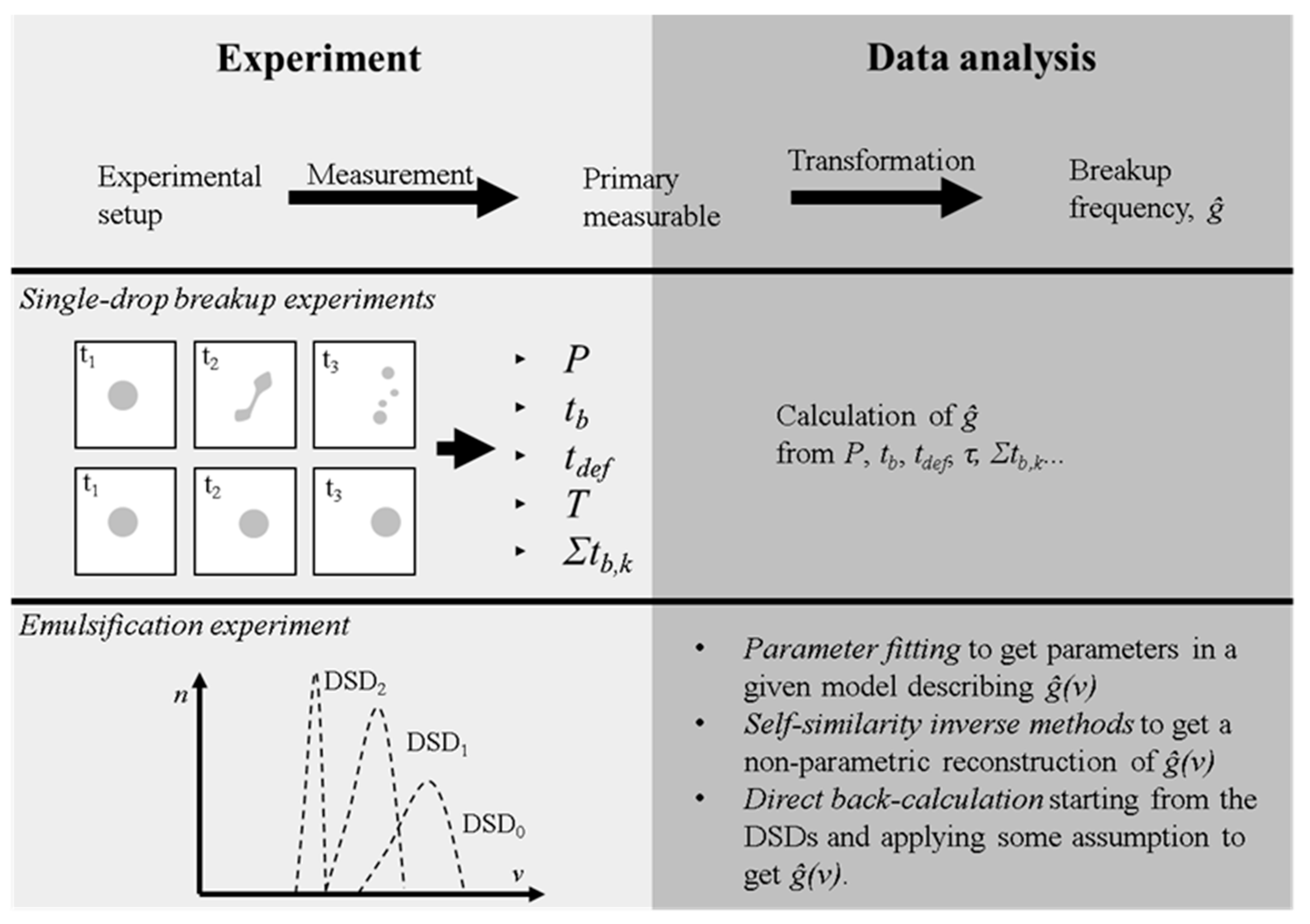
3. Classification of Methods

No methods have been presented for directly measuring the breakup frequency. Instead, all of the suggested techniques can be seen as consisting of two steps. First an experimental step, where an experimental setup is used to measure a ‘primary measurable’. Then, secondly, a data analysis step, where the primary measurable is used to estimate the breakup frequency. The upper pane of Figure 2 provides an illustration of the two steps involved in measuring the breakup frequency.

Two main types of studies estimating the breakup frequency can be seen in the literature, differing in terms of which approach they use in the experimental step. The first type uses specially constructed flow setups allowing for the injection of single drops, and then directly observes the fate of each drop as it passes through the turbulent zone. Typically, this is achieved by high-speed imaging in flow cells with optical access. Several properties of the breakup process can be directly observed from such a setup; for example, the probability of breakup for drops of different diameters and the average breakup time. These studies typically use their primary measurables to estimate the breakup frequency in a fairly direct way (see the illustration in Figure 2). The directness in calculating the fragmentation frequency is often seen as the method’s main advantage. This approach has been used for measuring both global and regional breakup frequencies, and will be referred to as ‘single drop breakup studies’ in this review. This class of methods is discussed further in Section 4.

The other type of technique uses an altogether different approach, starting from a standard emulsification experiment. The typical emulsification experiment consists of preparing a pre-emulsion, feeding it to the turbulent emulsification device of interest, and sampling the resulting DSD. These approaches typically require that the DSD is sampled several times during the emulsification process, e.g., by repeatedly passing the emulsion through a high-pressure homogenizer or inline rotor-stator mixer and sampling after each passage [33,44], or sampling the emulsion at several time-points when processing it in a stirred batch system [31,41]. The obtained sets of DSDs are then used to estimate the breakup frequency using transformation (see the lower pane in Figure 2). All investigations based on emulsification experiments will result in global estimates of the breakup frequency, as a consequence of using DSDs (which are inherently global) as the experimental input.

Three main types of breakup frequency determination methods using emulsification data can be seen in the literature, differing in terms of which transformation they apply in the data analysis phase. The first (and oldest) approach involves specifying the breakup frequency as a semi-empirical model with fitting constants, solving the forward PBE-problem formulated in the standard form (Equation (4)), and using non-linear regression to determine the fitting parameters of g*(v). This approach will be referred to as ‘parametric determination’ and is discussed in Section 5.

The second approach suggested for estimating the breakup frequency from emulsification data is the use of non-parametric inverse PBE methods—mathematically rigorous techniques that only require the fragmentation process to be ‘self-similar’. This approach will be referred to as using ‘inverse self-similarity based methods’ and is discussed in detail in Section 6.

The third and last approach consists of introducing additional assumptions for the fragmentation process, allowing the breakup frequencies to be obtained more directly from the DSD data. This approach will be referred to as ‘direct back-calculation’ and is discussed in more detail in Section 7.

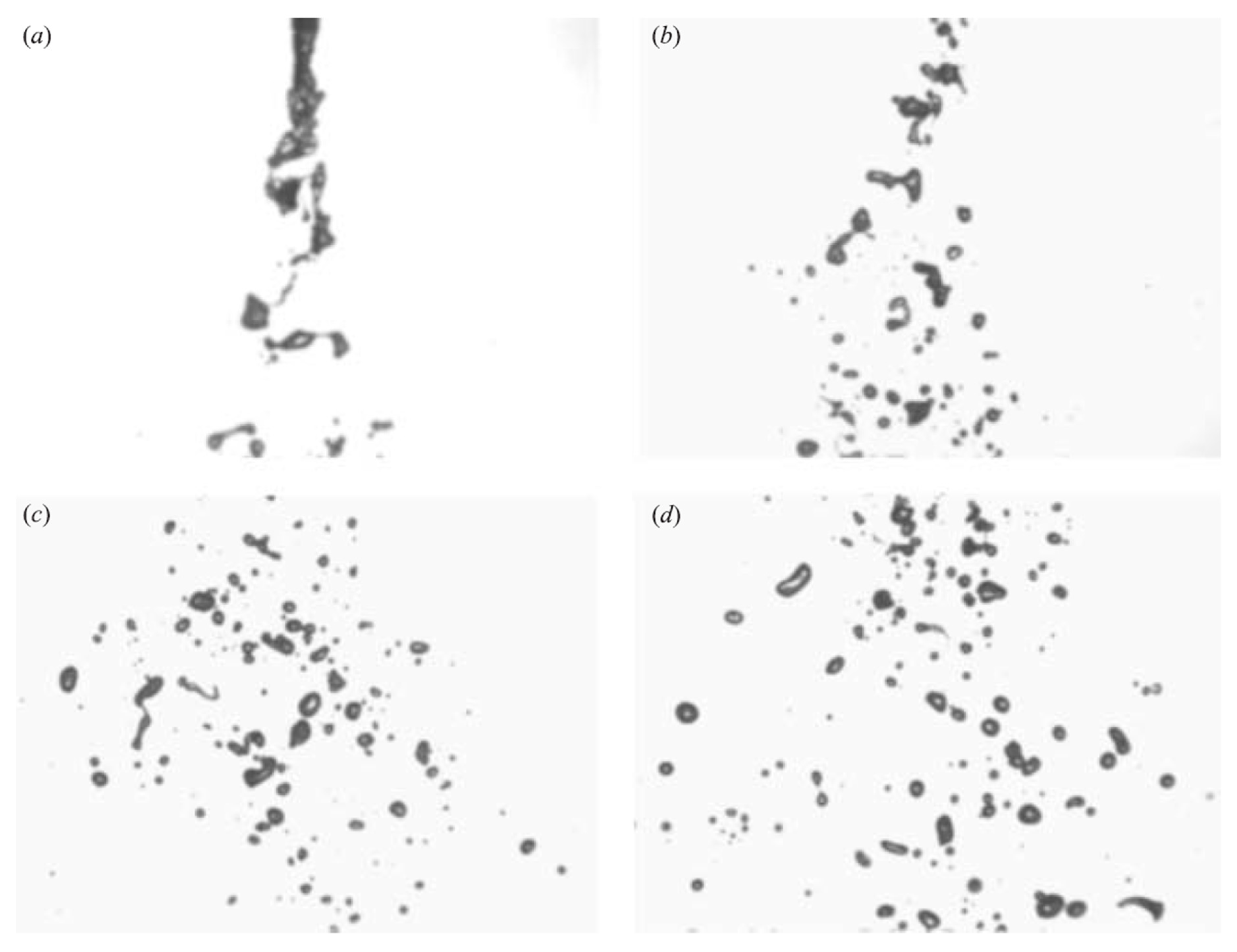
4. Single Drop Breakup Experiments

4.1. The Typical Experimental Setup

A schematic view of the typical single drop breakup experiment can be seen in Figure 3: A drop is formed (e.g., using a capillary injection needle) and is introduced into a specially designed turbulent flow geometry allowing for optical access. A high-speed camera is set up to take a series of images of the drop in rapid succession, as schematically illustrated in Figure 3A–C. If the optical conditions are appropriately set (see the discussion in Section 4.4), a series of sharp images are obtained. When combining these types of images (see Figure 3D for a schematic view and Figure 4 for an example from an actual study), this allows for the direct determination of several quantities describing the breakup, such as

• The number of drops fragmented before exiting the zone;
• The percentage of drops fragmented upon passing the zone;
• The number of daughter drops formed per breakup;
• The size distributions of the daughter drops.

Despite the difficulties in designing, setting up, and analyzing the data from such experiments, a growing number of single drop breakup visualizations have been published for various turbulent flows. However, it should be noted that only a smaller subset of these high-quality single drop breakup visualization studies have attempted to estimate the breakup frequency. These studies are summarized in

Table 1. Summary of the single drop breakup experiments that have attempted to measure the breakup frequency.

Ref.	Application	Flow	Re (103)	D0 [µm]	N0 [-]	N1 [-]	tdef?	tb?	P?	Nbr. frag. ?	Frag PDF?	Trans-Formation
[47]	Stirred tank	Flow near the impeller	5	1000–4000	543	?		YES		YES		A
[48]	Rotating disc contractor		?	2000–5000	?	?			YES			B
[49]	Pulsed sieve-plate column		?	?	?	?			YES			B
[14]	Stirred tank	Wake of impeller blade	20–40	500–3500	~4 500	~3 000		YES	YES			C
[50,51]	Static mixer	Near uniform intensity	7	1000	300	?		YES	YES	YES	YES	C
[13]	Stirred tank	Flow near the impeller	21–29	2500–3400	457	?		YES	YES	YES	YES	C
[6,29]	Rotor-stator mixer	Jet from a stator slot	20	70–550	285	56	YES		YES	YES		C’
[12]	Nozzle jet	Jet	6–26	2000–5000	?	1089				YES	YES	D

Re: Reynolds number; D₀: injected (initial) drop diameter; N₀: total number of drops injected; N₁: total number of drop breakup events monitored; t_def?: does the study measure the deformation rate?; t_b?: does the study measure a breakup time?; P?: does the study measure the breakup probability?; Nbr. frag?: does the study measure the number of fragments formed?; Frag. PDF?: does the study measure the fragment size distribution?; Transformation: method used to estimate the breakup frequency from the primary measurements (see Section 4.2); ?: dData not available in the original study.

(a discussion of the single drop breakup visualization studies not measuring the breakup frequency is beyond the scope of this review, and can be found elsewhere [6,45,46]). Section 4.2 discusses the principally different approaches these studies have used to calculate the breakup frequency from the variables directly observed. Section 4.3 briefly summarizes the setups of the individual studies and Section 4.4 discusses experimental considerations.

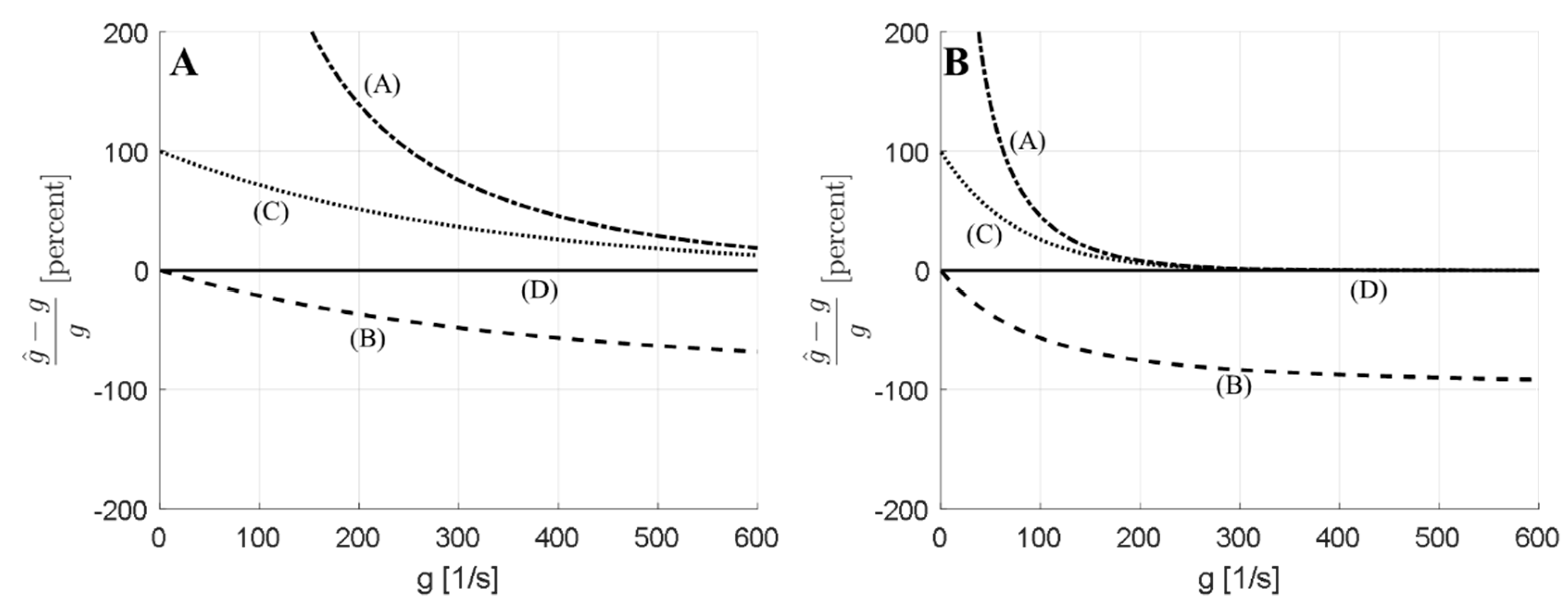
4.2. Methods for Estimating the Breakup Frequency

As noted by Vejražka et al. [12], the breakup frequency is not (as opposed to the breakup probability or breakup time) directly observable in a single drop breakup experiment. Some transformation of the primary measurables is always needed. By comparing the studies presented in Table 1, five principally different methods of how to use the primary measurements to calculate the breakup frequency can be identified (marked by A-D in the last column of Table 1).

The first suggestion was made by Hančil and Rod [47], who estimated the breakup frequency as the inverse of the (average) breakup time (t_b):

$$g_A=\frac{1}{t_b}.$$

(13)

The authors [47] did not provide a motivation for why Equation (13) should be a valid estimate of the breakup frequency. However, Equation (13) could be understood in terms of a suggestion by Ramkrishna [20] (p. 51), by describing the breakup frequency as the reciprocal of an average ‘survival time’.

Another suggestion was made by Gourdon and Casamatta [49], who estimated the breakup frequency by combining the breakup probability (P) and hold-up time (τ) (i.e., the average time a drop has spent in the turbulent zone):

$$g_B=P\cdot \frac{1}{\tau }.$$

(14)

The same method was used in a later study [48].

The third suggestion is to estimate the breakup frequency as the breakup probability multiplied by the inverse of the average breakup time:

$$g_C=P\cdot \frac{1}{t_b}.$$

(15)

This description of the breakup frequency was first introduced by Coulaloglou and Tavlarides [41] in modeling the breakup frequency. However, it has also been extensively employed in experimental studies for estimating the breakup frequency from empirical data [13,14,46,50,51], making it the most commonly used method.

As discussed by Solsvik et al. [46], the term ‘breakup time’ has not always been clear in previous studies, since breakup is often a multi-step process where deformation, fragment formation, and droplet relaxation can occur several times, as a fragment formed in one breakup event is fragmented again before exiting the investigated turbulent zone. Therefore, one can define the breakup time as the time at which the first droplet detaches from the mother drop, or as the time until the mother drop has been broken up into the final number of fragments. This introduces some additional variations into the suggestions of how to estimate the breakup frequency from experimental data, since different studies use different definitions of t_b when evaluating Equation (15).

Another slight modification to Equation (15) was used by Karimi and Andersson [29], who argued that since drop deformation is the critical step giving rise to fragmentation, the deformation time should be used in the denominator instead of the breakup time:

$$g_{C^{\prime }}=P\cdot \frac{1}{t_{def}}.$$

(16)

The final suggestion of how to estimate the breakup frequency from single drop breakup data was suggested by Vejražka et al. [12], who calculated the breakup frequency as the total number of observed breakup events divided by the total time spent in the turbulent zone (until breaking or exiting) of all observed drops:

$$g_D=\frac{\mathrm{Number}\mathrm{of}\mathrm{breaking}\mathrm{drop}}{\mathrm{Total}\mathrm{time}\mathrm{spent}\mathrm{in}\mathrm{zone}\mathrm{of}\mathrm{all}\mathrm{drops}}=\frac{N_0-N_1}{\tau \cdot N_1+{\displaystyle \sum t_{b,k}}},$$

(17)

where N₀ is the number of injected drops, N₁ is the number of surviving drops, and Σt_b,k denotes the sum of all individual breakup times.

Table 1 summarizes the different studies that have attempted to measure the breakup frequency from single drop breakup experiments, showing which of the methods (A–D) each study used. Two things can be noted from this comparison. First, with the exception of method A, all methods require that statistics are obtained not only for breaking drops, but also for non-breaking drops (e.g., by depending on the relative number of breaking drops). Therefore, a large number of drops need to be tracked for each experimental conditions, which makes this type of investigation time consuming.

Secondly, as can be seen by comparing the different methods (Equations (13)–(17)), there are several different suggestions of how to calculate the breakup frequency from drop breakup visualization data. Also note that the expressions are not in agreement which each other—subjecting the same single drop breakup dataset to each of the five methods would give rise to systematically different estimations of the breakup frequency (for example, Equations (14) and (15) differ when all drops do not break exactly at the exit, and Equations (13) and (14) differ as soon as drops entering the turbulent zone survive without breaking).

The conflicting estimates imply that some of them are invalid, at least if one does not see each study as estimating a principally different ‘frequency’ (which, as discussed in Section 2.1, is an unfruitful approach, since the overall objective in all of these studies has been to obtain a breakup frequency that can be used to make predictions using the PBE). Ref. [12] is the only study providing proof that their transformation (method D, Equation (17)) results in a breakup frequency that complies with the PBE. However, a recent contribution [52] subjected all four models to a series of comparisons of analytical solutions to the PBE, as well as numerical simulations of the PBE. These investigations show that methods A, B, and C are invalid estimates of the breakup frequency; the breakup frequency estimated from these equations would not be able to reproduce the shift in the DSD seen in the experiments when incorporated in the PBE [52]. However, each of the methods (A, B, and C) provide an estimate that tends towards the true value if the breakup frequency is either very high (A and C) or very low (B) [52]. Figure 5 shows the relative systematic error that is obtained when using each of the methods (A, B, C, and D) to estimate the breakup frequency from a single drop breakup experiment, assuming that the hold-up time is either 5 or 20 ms and constant throughout the turbulent zone, using the methodology described in Ref. [52]. As can be seen in Figure 5, the systematic errors are substantial if an inappropriate method is used in the data analysis stage, even when the experimental setup is optimal and the primary measurements (breakup probability and breakup time) are determined with a high reliability and validity.

Note that this finding—that many of the methods previously used to calculate the breakup frequency from single drop breakup experiments give rise to systematic errors—makes it difficult to compare results from different studies. However, from a methodological perspective, it is still interesting to discuss under what conditions experiments have been performed (Section 4.3), in order to discuss directions for future investigations and guidelines for experimental setups (Section 4.4).

4.3. Individual Studies—Experimental Setup

This section summarizes, briefly, the experimental conditions used in the individual studies employing the single drop breakup visualization approach to measure drop breakup.

Hançil and Rod [47] conducted one of the first single drop breakup visualization experiments by studying the fragmentation of oil drops (~1–4 mm) in the turbulent flow created close to an impeller in a stirred tank. Although the (global) breakup frequency was also measured, the main focus was on discussing the number of fragments formed per breakup and the distribution of fragment sizes.

Gourdon and Casammata [49] investigated the fragmentation of oil drops in a pulsed-sieve plate column. The main objective was to characterize the mass transfer, but the (global) breakup frequency was also measured. This study did not use a high-speed camera setup for determining if a drop breaks or not (as is typically the case for methods in this class). Instead, Gourdon and Casammata [49] equipped their flow setup with a photoelectric cell, making it possible for them to detect and measure the size of each injected drop.

Schmidt et al. [48] mainly studied mass transfer in a disc rotating extractor, but also measured the (global) breakup frequency for oil drops (2–5 mm). The study used the same photoelectric cell setup as in ref. [49].

Andersson and Andersson [50] reported one of the first studies specifically designed to measure the (global) breakup frequency in an emulsification device, and also compared the obtained breakup frequency to a new breakup frequency model [51]. The experiments were conducted on a ‘novel reactor’ [53], designed to give a near-constant turbulent intensity, and used high-speed photography to study the drops. Detailed investigations of the drop deformation and number of fragments formed were reported. The breakup frequency estimations were presented in a theoretical follow-up paper [51]. The methodology applied for estimating the breakup frequency from the experiments was not described in great detail.

Maaß and Kraume [14] studied the breakup of oil drops in the wake of an impeller blade, in an experimental model of a stirred tank equipped with a Rushton turbine. Detailed data was reported in terms of breakup probability and breakup time probability distributions. These results were also used to estimate the (global) breakup frequency.

Solsvik and Jakobsen [13] also studied breakup in a stirred tank, but using air bubbles instead of emulsion drops. However, this study also reported detailed data on the breakup probability and breakup time, discussed the probability of multiple fragment formation, and estimated the (global) breakup frequency.

Ashar et al. [6] conducted single drop breakup visualization on a turbulent jet created in the stator slot of a rotor-stator mixer, and performed a comprehensive investigation of the fragments and deformation time-scales. The breakup frequencies were calculated and reported in a follow-up study [29].

Vejražka et al. [12] measured the fragmentation of oil drops in an asymmetrical jet, combining investigations of the fluid flow and turbulence with single drop breakup visualizations. This was also the first single drop breakup study attempting to measure regional breakup rates, by dividing the turbulent zone of interest into ‘windows’, each narrow enough to show a near constant dissipation rate of turbulent kinetic energy, and then applying their measurement technique on each window separately.

4.4. Experimental Considerations

The clear majority of single drop breakup experiments use high-speed photography to visualize breakup (although exceptions exist [48,49]). Two conditions need to be fulfilled in order to obtain reliable and valid estimates of breakup frequencies from a single drop breakup visualization experiment. First, the transformation used to calculate the breakup frequency needs to be valid (see the discussion in Section 4.2). Secondly, the breakup visualizations must be designed in such a way as to allow for an accurate determination of the primary measurables, such as the breakup probability and breakup time.

Setting up the right optical conditions for a high-quality drop breakup visualization study is challenging [54]. However, the optical setup is typically not described in great detail in the published papers (see

Table 2. Setup and optical considerations presented in previously reported single drop breakup visualization studies. For each of the studies, the specified experimental conditions, the steps taken to ensure a sufficient contrast in visualization images, and the high-speed camera settings are shown, together with four calculated properties added as suggestions of relevant guidelines for future investigations (see Section 4.4 for a discussion).

Ref.	Studied Conditions			Contrast		Camera			Calculated Properties
	U [m/s]	tb [ms]	D0 [µm]	Contrast-Enhancer	Lighting	Shutter Time tsh [µs]	FPS	Δx [µm/pixel]	Pixels Per Drop.diam (D0/Δx) [-]	Movement Per Shutter Time in % of a D0 (tsh·U)/D0 [-]	Movement Per Shutter Time in Pixels (tsh·U)/Δx [-]	Images Per Breakup (FPS·tb) [-]
[47]	0.4	>3000	1000–4000	None	?	?	?	?	?	?	?	?
[14]	1–3	~12–34	500–3500	‘Black dye’	?	?	?	?	?	?	?	?
[50,51]	7 *	~3–11	1000	None	Front light + reflector behind	10–100	4000	18	60	7–70%	4–40	10–40
[13]	2	15–25	2500–3400	None	Halogen lights + light diffuser	?	1000	10 **	100	?	?	40–90
[6,29]	4	~1.5–3.0	70–550	None	Halogen light 5 × 50 W	5	2800–3000	25	3–20	3–30%	0.8	4–9
[12]	0.3	?	2000–5000	None	?	170–250	2000	92.5	20–50	1–3%	0.6–0.8	?

(*) Estimated from scaling with the volumetric flow using data from another paper on the same reactor [53]. (**) Estimated assuming that the reported smallest drop (which is given in the paper) is 10 pixels in diameter. (?) Data not available in the original study.

for a summary). This section summarizes some of the methodological discussions presented in previous studies, focusing on challenges and solutions for providing accurate breakup visualizations, in order to give guidelines for future investigations.

The challenge in setting up a single drop breakup visualization study is the need to obtain sharp and well-resolved images of the deforming and breaking drop. This is of special importance since a clear majority of the single drop breakup visualizations use image analysis software to automatically calculate breakup probabilities and breakup times for the large number of drops required to obtain statistically converged results. Despite the possibilities to employ enhancement algorithms, such as edge detection or background subtraction, high-quality primary data is essential. Based on the studies in Table 2, four factors can be identified as critical for obtaining high-quality visualizations:

• Sufficient resolution of the drops to accurately measure the size of fragments;
• Sufficiently large depth of field (DOF) to make sure the drop does not become blurry;
• Sufficiently high contrast between the drop and continuous phase;
• Sufficiently fast camera.

Each factor is treated in a separate subsection below. Since there have been no systematic investigations (theoretical or experimental) of what would be sufficient conditions for obtaining an acceptable image quality, the focus here will be on reporting what conditions have been used in previously published studies. However, since all of these have reported sharp images, one could also see these as indications of conditions that are expected to give an acceptable quality in future investigations.

4.4.1. Image Resolution

The drops investigated are typically small (~1 mm), and the fragments are even smaller. Moreover, the images recorded by a digital high-speed camera have a limited resolution given by the sensor density on the CCD chip. This will set the limit in terms of the size fragments that can be observed in a visualization experiment and is often adjusted by equipping the high-speed camera with magnifying lenses (e.g., extension tubes and macro lenses). However, as discussed below, increasing the magnification also has other negative side effects on the image quality and a suitable compromise must be made. Table 2 summarizes and compares the pixel resolution (number of pixels divided by the initial diameter of the drop, see the illustration in Figure 6), showing that previous studies have found it useful to have a resolution of roughly between 10 and 100 pixels per mother drop diameter (here, it could be noted that the pixel resolution of the smallest fragment is probably a better basis for comparing the resolution. However, the studies in Table 2 do not report the smallest fragment size, and thus, such a comparison is not possible at this point).

4.4.2. Depth of Field (DOF)

The depth of field (DOF) is defined as the width of the layer (in the direction orthogonal to the image field) which is in sharp focus (see Figure 6A). A major challenge when attempting to focus on a drop subjected to a turbulent flow is that there will always be some out-of-plane movement (due to the stochastic nature of a turbulent flow). This becomes problematic if the DOF is narrow, since the drop will move in and out of focus. A rough approximation of the depth of field is given by the Berek formula [7]:

$$DOF=\frac{\lambda }{2A_N^2}+\frac{R_P}{M\cdot A_N^{}},$$

(18)

where λ is the wavelength of the light, A_N is the numerical aperture, M is the image magnification, and R_P is the resolving power of the lens. Consequently, the high magnification typically required for capturing small fragments gives rise to a lower DOF, thus increasing the risk of a drop which is initially in focus moving out of focus before it breaks or exits the turbulent zone under investigation.

Equation (18) also illustrates that the DOF strongly depends on the numerical aperture; reducing the amount of light entering the sensor will increase the DOF. Therefore, the solution used in single drop breakup visualization studies is to keep the aperture as small as possible and make sure to employ high-intensity lamps to provide enough light, often in the form of halogen lights (see Table 2).

4.4.3. Contrast

Another substantial challenge is obtaining a sufficiently high optical contrast between the drop and the continuous phase. This is generally more difficult to achieve when working with drops than bubbles, due to the relatively small difference in the refractive index between oil and water. Some studies have added dyes (e.g., Sudan black) to the oil phase, in order to increase the optical contrast [45], and another option is to add fluorescent molecules to the oil, e.g., Nile red [7], which also has the advantage of only fluorescing in the oil phase.

One concern relating to using dyes (fluorescent or not) is that these might influence the interfacial tension of the system, which is expected to have an effect on the fragmentation rate [26]; there is a risk that a drop with added dye breaks differently than a drop without dye, since it might then have a different Weber and Capillary number. Studies using dyes typically measure the effect on interfacial tension to discuss the extent of this effect [14]. This should be considered good practice for future investigations.

Another factor that has been used to increase the disperse to continuous phase contrast is the positioning of the light sources, and using reflectors and diffusors. However, the published studies rarely give details on how the setups were made (see Figure 1 in ref. [50] for an exception), making it difficult to discuss best-practice here.

4.4.4. Camera Speed

Two factors should be discussed in terms of the camera speed. First, the shutter time (also known as the exposure time) of the camera needs to be sufficiently short to give a sharp drop. If the shutter time is too long, the drop will have moved several pixels during the exposure, resulting in an apparent elongation of the drop (see the schematic illustration in Figure 6B). Some indication of what shutter time is needed can be obtained by comparing meaningful scaling with the published studies. If t_sh denotes the shutter time and U denotes the drop velocity, each point in the drop has moved a distance (t_sh·U) during the exposure. This distance should be short in comparison to the pixel resolution, Δx, and in relation to the drop diameter, D₀, in order for the drop not to appear artificially elongated. Table 2 compares the studies in terms of these dimensionless numbers. Since many of these studies conducted experiments under a range of conditions (e.g., different fluid velocities) and reported shutter times as a span (rather than as a value for each experimental condition), it is difficult to give an exact value for these dimensionless numbers. However, assuming that conditions were set so as to reach the lower limit of the interval, shutter times resulting in a drop motion of a few percentages compared to the mother drop diameter or, alternatively put, a shutter time giving a drop motion of no more than 4 pixels, seems to be what has provided acceptable results in previous investigations.

The second factor related to the camera speed is the framerate of the camera (FPS), which must also be sufficiently high. The framerate determines how many images can be captured during the breakup process, and should be as high as possible to obtain breakup times with a high resolution (remember that t_b is a factor in most of the equations used to estimate the breakup frequency from experiments). From the summary in Table 2, between 4 and 90 images per breakup haven been used in previously published investigations.

5. Parametric Determination

5.1. The General Approach

Using the PBE to predict the DSD resulting from turbulent breakup is uncomplicated once the breakup frequency (and fragment size distributions) is known—a variety of numerical solution schemes are available [20,42,43]. However, the inverse process of estimating the kernels from the DSD is an ill-posed problem unless a special assumption or transformation is introduced [20]. All of the emulsification data-based approaches (see Figure 2) are different attempts of ‘regularization’, i.e., attempts to add information to the problem in order to make the inverse problem solvable.

The parametric determination method is, arguably, the easiest to implement. This approach starts from the fact that many of the oldest breakup frequency models were formulated based on the scaling relationship, which included one or several parameters that needed to be determined experimentally [41]. The parametric determination methods employed for measuring breakup frequencies run forward simulations (calculating the resulting DSD from the initial DSD and a set of breakup frequency parameters), compare the measured to predicted DSDs, and repeat this until finding the set of parameters that best reproduces the experimental DSD. This can be done manually (more common in earlier studies [41]) or automatically using a non-linear regression algorithm (more common in the last few decades [24,55]).

Since standard methods are available—both for solving the discretized PBE and for non-linear regression—this method is relatively easy to implement. Moreover, the computational time required for fitting the constants is negligible on a standard laptop. This has made the parameter fitting methodology popular. Specific examples of the technique are given in Section 5.2, and a critical discussion can be found in Section 5.3.

5.2. Individual Studies

Since the number of studies using this approach is exceedingly large (and the methodology for obtaining the breakup frequency is similar between the studies), only a few typical and influential examples are given below.

Coulaloglou and Tavlarides [41] measured the evolution of the DSD of an emulsion processed in a tank fitted with a turbine impeller (190–300 rpm). A two-parameter breakup frequency model and a fragment size distribution (with two additional parameters) were fitted to the experimental data. The experiments included disperse phase volume fractions in the range of 5–15%. However, only the lowest volume fraction data was used for determining the four fitting parameters. This breakup model was then combined with an experimentally verified (obtained from an independent experiment) coalescence model and the model predictions were compared to the experimental data for higher volume fractions, showing good agreement between modeled and measured evolution in the average drop diameter.

Konno et al. [56] suggested a new breakup frequency model with two fitting parameters (together with a parameter-free fragment size distribution and a coalescence model with two fitting parameters). The evolution of the DSD with time, in a batch tank fitted with baffles and an impeller (60–450 rpm), was measured and the four fitting parameters were determined by comparing modeled to measured DSDs (presumably, manually, and based on the entire dataset).

Tsouris and Tavlarides [55] suggested a new breakup frequency model, with only one fitting parameter (together with a parameter-free fragment size distribution and a coalescence frequency model with one fitting parameter). Emulsification experiments were run on a baffled batch tank equipped with a Rushton impeller (270–330 rpm) and a disperse phase volume fraction of 10–30%. The two fitting parameters were determined using least square analysis (presumably using the whole experimental dataset).

Raikar et al. [23] used parametric determination to analyze emulsification in a laboratory-scale high-pressure homogenizer run at different pressures (25–125 MPa), volume fractions of oil (5 or 10%), and emulsifier concentrations. In the base case, a semi-empirical breakup frequency model with four parameters was suggested (and used together with a fragment size distribution model with one parameter and a coalescence model with two parameters). The four breakup frequency parameters were determined using a constrained least square optimization algorithm, from the experiments run at the lowest volume fraction (assumed to be free of coalescence). In order to improve the fit between the modeled and measured DSDs, the authors investigated several model developments. The largest improvement was obtained when including the fitting constant in the fragment size distribution in the procedure, thus increasing the number of fitting constants (for the case with only fragmentation present) to five.

Aziz and Taweel [32] investigated emulsification in a reactor/contractor with different screen sizes (mesh size of 0.8–1 mm) and measured the DSD as a function of time. Breakup and coalescence was assumed to progress according to Coulaloglou and Tavlarides’ [41] model and the four fitting parameters were determined by least square analysis based on the data measured at one of the screen sizes. The other two screen sizes were used to test the model, and a comparison of the modeled and measured average drop size for these two additional screen sizes showed a good agreement.

Riberio et al. [57] investigated emulsification in a batch tank equipped with baffles and a Rushton turbine (~100 rpm). The experimentally measured data was fitted to both Coulaloglou and Tavlarides’ [41] breakup/coalescence models (in total, four fitting constants), as well as to other suggestions of coalescence frequency models, using a non-linear optimization algorithm based on least square minimization. Riberio et al. [57] also pointed out that the estimated values of the fitting parameters depend on whether number-based or volume-based DSDs are used in the minimization routine, and suggested a method with weights based on the class volume to obtain a suitable compromise.

5.3. Critique

Several objections have been raised against parametric determination. One clear disadvantage of the approach is that one needs to assume that the general shape of the breakup frequency is already known, except for a few parameters. This is a rather severe assumption in light of the discussion in the theoretical modeling literature, where there is a large number of highly dissimilar breakup frequency models [26,27,28]. The standard argument against this critique—in defense of parametric determination—is that obtaining a good fit between measured and modeled DSDs would suggest that the model is actually a valid representation of the fragmentation process. As can be seen in Section 5.2, many studies find that it is possible to obtain a small model residual.

However, a close fit between a fitted and measured DSD could also, at least theoretically, be the effect of overfitting. It is well-known that a small sum of square residuals can always be obtained in regression analysis if using a large enough number of fitting constants, even if the underlying model is not physically relevant [58,59]. This is of special importance in parametric determination of the breakup frequency since the number of fitting parameters is typically large (2–5) and close to the number of parameters with which one could obtain a good fit to almost any shape using a black-box model [60].

The standard response to the overfitting critique is to divide the experimental data in two, forming a ‘training set’ used to fit the model parameters, and a ‘hold-out set’ (sometimes referred to as a ‘test set’ or ‘sample set’) used to test the model [58]. As seen in the list of previous investigations presented above (Section 5.2), some studies have used this approach [23,41] to argue that their good fit between modeled and measured data is not due to overfitting.

Another challenge, often overlooked, when using parameter fitting techniques to measure the breakup frequency, is that the fragment size distribution (including the number of fragments formed per breakup) must also be known and explicitly specified. This is a severe complication since there are as many varying fragment size distribution models as there are breakup frequency models [26]. Again, one could argue that a small residual would suggest that the right f* (or at least an approximation of the true one) has been specified. However, there is nothing guaranteeing that the breakup frequency and fragment size distribution used in one of these studies represent the only model able to give a small residual. Additionally, if there are several different combinations of parameter values or several different functions g* and f* able to approximate the DSD evolution, how could one be sure that what has been obtained in a parametric determination is a physical breakup frequency, and not merely a black-box fitting?

Comparisons have showed that different authors studying similar systems get rather different best-fit parameters, even when fitting the same semi-empirical models (e.g., see the comparison in ref. [61]). This is problematic. It the semi-empirical models used when conducting parametric determination of the breakup frequency were actually good descriptions of the fragmentation physics, one would expect the parameter values to be universal. Moreover, the observation that the parameters depend on which form of the DSD is used in the optimization process [57] also suggests similar problems with this approach.

In summary, the parametric determination methods have been used extensively, which is understandable since they are relatively easy to use and are often able to show a close fit to measured DSDs. However, the technique also suffers from several shortcomings, especially in terms of the risk of overfitting and the severe assumptions imposed on the shape of the breakup frequency and fragment size distributions.

6. Self-Similarity-Based Inverse Methods

6.1. General Approach

As noted in Section 5.1, the inverse problem—calculating the breakup frequency, g*, from the known evolution of the DSD—is generally an ill posed problem. However, starting in the late 1970s, Prof. Ramkrishna and co-workers suggested a method allowing for a non-parametric reconstruction of the breakup frequency (and the cumulative fragment size distribution), provided with what appears to be a fairly mild assumption; that the fragmentation process is characterized by ‘self-similarity’.

6.2. Self-Similarity

By definition, a self-similar fragmentation process gives rise to a DSD that is invariant, i.e., allowing all of the DSDs (obtained after different numbers of device passages or processing times) to be described by a single curve after an appropriate transformation of variables. This transformation is from the two physical variables–drop volume, v, and time, t—to a self-similarity variable X. More specifically, a fragmentation process is self-similar if it is invariant under the transformation [20],

$$X=\frac{g(v)}{g(v_0)}t,$$

(19)

where g(v₀) is the breakup frequency for a nominal drop volume v₀. Figure 7A,B illustrates the concept of self-similarity by showing the cumulative DSDs arising from two different combinations of (global) breakup frequency functions and fragment size distributions (based on solving the forward PBE, Equation (4), for the different kernels). One of the examples in Figure 7A is characterized by self-similarity (the cumulative DSDs collapse), whereas the other (Figure 7B) is not (the curves do not collapse).

It has been shown [62] that self-similarity is equivalent to a relationship existing between the breakup frequency and the cumulative breakup function, G(v|v’) [62], so that,

$$G(v|v^{\prime })=\gamma \left(\frac{g(v)}{g(v^{\prime })}\right),$$

(20)

for the function γ(u), with u = g(v)/g(v’).

If the kernels (g* and f*) would be known with certainty, it would be easy to test whether the fragmentation process was self-similar (by using Equation (20)). However, the kernels are generally unknown and it is not trivial to see from Equation (19) or Equation (20) if self-similarity is a severe or mild assumption. Moreover, there is of yet no general consensus as to if this is a property generally characterizing turbulent emulsification.

6.3. The Three Steps Employed for Calculating the Breakup Frequency

Reconstructing the fragmentation frequency with self-similarity-based inverse methods involves three steps [20,63,64]:

• Testing if the fragmentation process is self-similar;
• Calculating the shape of the scaled breakup frequency through a direct integration of experimental data;
• Determining the scaling and cumulative fragment size distribution through a non-linear regression on the self-similar PBE solution expanded in terms of basis functions.

Starting with (1), testing when a fragmentation process displays self-similarity is not trivial given the measured DSDs. The procedure suggested by Sathyagal et al. [63] starts from the empirically measured cumulative DSD. First, the cumulative DSDs are plotted at different times (see Figure 8). Then, an iso-F-value is chosen, F_iso,k, and the limiting drop volume at which F has reached this value at different times is collected in a vector v_k. The corresponding times are collected in a vector t_k. Figure 8 shows how the first two elements of the vectors v_k and t_k are formed. This is then repeated for another iso-F value (e.g., F_iso,1 = 0.2, F_iso,2 = 0.6 and F_iso,3 = 0.8, …).

Narsimhan et al. [62] showed that self-similarity will imply that when plotting ln(v_k) versus ln(t_k), this will result in parallel lines, or equivalently, that the arch lengths of the x = ln(v_k) versus ln(t_k) curves will collapse on a single curve. Sathyagal et al. [63] tested for similarity by visually inspecting if these arc-length curves collapsed or not, and this has emerged as best-practice. Figure 7C,D illustrates the procedure by showing arc-length curves, s(x), for the two theoretical cases discussed in Section 6.1. As can be seen in Figure 7, the first case (Figure 7C) (representing self-similar fragmentation) shows collapsing arc-length curves, whereas the second case (Figure 7D) (which is not self-similar) does not collapse.

The second step (2) in using the inverse self-similarity method to measure the breakup frequency is a straight-forward integration of the curve determined by the (v_k, t_k) pairs:

$$\frac{\widehat{g}(v)}{g(v_0)}=\exp \left[-{\displaystyle \underset{\ln v_0}{\overset{\ln v}{\int }}{\left(\frac{\partial \ln t}{\partial \ln t}\right)}_{F}d\ln v}\right].$$

(21)

Equation (21) gives the breakup frequency (discretized with the resolution given by the resolution in the DSD) except for a scaling constant, g(v₀), describing the breakup frequency at the reference volume v₀ (see Equation (19)).

The third step (3) determines this constant and at the same time provides a non-parametric reconstruction of the cumulative fragment size distribution, G (see Equation (12)). This last step is slightly more complicated, and there are two different influential suggestions for conducting it [63,64]. Both methods start from realizing that under the self-similarity transformation (Equation (19)), the cumulative DSD, F(v,t), transforms to f(X). It can be shown that the PBE (Equation (4)) in terms of these transformed variables takes the following form [63]:

$$X\cdot f^{\prime }(X)={\displaystyle \underset{u=0}{\overset{1}{\int }}\frac{X^2}{u^3}{f}^{\prime }\left(\frac{X}{u}\right)\cdot g(v_0)\cdot \gamma (u)du}.$$

(22)

In brief, step (3) consists of determining g(v₀)·γ(u) by solving a discretized version of Equation (22). The left hand side of Equation (22) (which is known since X·f(X) is simply a transformation of the measured DSDs), is expanded in terms of gamma distributions and the expansion coefficients are determined directly from the experimental data. For the last step, the two methods differ. The original method [63] expanded g(v₀)·γ(u) using three modified Jacobi polynomials with proportionality constants, a₁, a₂, and a₃. This translates Equation (22) into a nonlinear regression problem which can be solved for the constants a₁, a₂, and a₃. Once a has been determined, γ(u), and g(v₀) can be calculated, since γ(u) = 1 by definition (see Equation (20)). Combined with Equation (21), this gives a complete non-parametric estimation of the discretized breakup frequency, where the only assumption is that the fragmentation process is self-similar. A more comprehensive description of the method can be found elsewhere [20,63,65]. An alternative method was suggested by Kostoglou and Karabelas [64] after pointing out several shortcomings of the original method. This modified method expands g(v₀)·γ(u) in gamma functions, allowing the proportionality constants to be determined from non-linear regressions using the moments of the self-similar distribution. A more comprehensive description of the method can be found elsewhere [64,66].

6.4. Individual Studies

Narsimhan et al. [62] applied an early version of the approach to estimate the global breakup frequency when dispersing low volume fractions (0.1%) of drops (50–400 µm) of organic solvents in water using a stirred tank. The fragmentation was concluded (by looking at how well the DSDs collapse on one curve when treated with the self-similarity transformation) to show self-similar behavior.

Sathyagal et al. [63] primarily developed and standardized the procedure (see Section 6.3), but also reported data from an experiment of dispersing an organic solvent in a batch tank at a stirring rate of 500 rpm. However, the emphasis was more on showing the feasibility of the method than on characterizing the device, and consequently, no experimentally estimated breakup rates were given.

Sathyagal et al. [31] provided a more comprehensive follow-up study applying the method to drops (10–500 µm) of four different organic solvents with disperse phase viscosities ranging from 20 to 200 mPa s and running the impeller at different stirring rates (350–500 rpm). The results show (global) breakup frequencies that are monotonically increasing in drop diameter, impeller speed, and disperse phase viscosity. Self-similarity is found across all conditions.

O’Rourke and MacLoughlin [66] estimated the (global) breakup frequency for silicone oils (disperse phase viscosity 20–500 mPa s) in a stirred tank equipped with a Rushton turbine running at different impeller speeds. Drop diameters were in the range of 10–400 µm. A total of 63 emulsification experiments were carried out and self-similarity was observed in 38 of them (at least after excluding several emulsification times from each experiment). The authors note [66] that cases where the drops are large (for example, due to having a low dissipation rate of turbulent kinetic energy or a high disperse phase viscosity) are less likely to display self-similarity. The resulting breakup frequencies compared well to a power-law expression based on a turbulent Weber number.

6.5. Critique

The first requirement of a method claiming to determine the fragmentation frequency experimentally is a high validity. Both versions of the method [63,64]) show that their inverse self-similarity methods are valid in the sense that they are able to reproduce a set breakup frequency when fed with theoretical data from a self-similar set of kernels that are noise-free.

As mentioned above, there is no consensus on to what extent the self-similarity assumption is actually fulfilled in emulsification devices. Individual studies (Section 6.4) often find that most setups are accurately described by self-similarity. However, the range of experimental conditions is still rather small and is limited to a stirred tank. Moreover, the most comprehensive experimental investigation [66] reported that approximately 40% of their experimental conditions did not display self-similarity, and that almost none of them did so when including all of the experimentally measured DSDs.

The second concern is to what extent the method is also reliable, i.e., how sensitive the method is to small imperfections in the measured DSD data. Raikar et al. [65] subjected the original inverse self-similarity method [63] to an extensive numerical investigation by feeding the algorithm with synthetic data from four cases (from a self-similar fragmentation process), each corresponding to more realistic cases, as would be seen in an experiment: A noisy DSD, a skewed DSD, a DSD with artefacts due to dust particles, and a binned DSD. Although Raikar et al. [65] (p. 7434) remained optimistic regarding the usefulness of the approach, the authors concluded that the approach gives rise to ‘significant errors for most of the cases considered’ when allowing for non-ideal data. The research group continued publishing a number of studies on the modeling and determination of breakup frequencies. However, each of these studies used parametric determination (Section 5) instead of inverse self-similarity analysis [23,24], suggesting that the researchers were discouraged from continued investigations with this method by their in-depth investigation of its reliability.

No comprehensive investigation of the reliability of the other most widely known methods for measuring the breakup frequency using inverse self-similarity analysis [64] has yet been presented. However, O’Rourke and MacLoughlin [66] reported this version of the method to be relativity insensitive to measurement uncertainty, at least when only using two gamma functions in expanding the fragment size distribution.

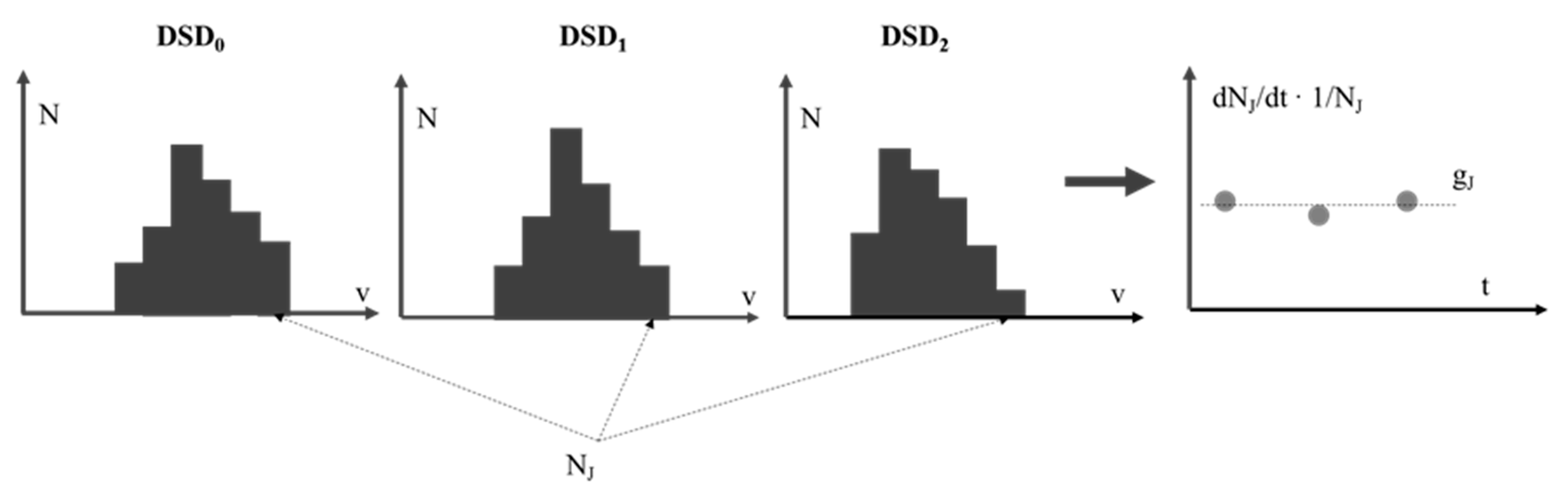
7. Direct Back-Calculation

7.1. General Approach

This class contains methods that do not use the specific inverse algorithms discussed in Section 6, but propose other attempts to calculate the breakup frequency more directly using simplifying assumptions. Consequently, the methods in this class are more diverse. Another difference is that the inverse self-similarity-based methods form a framework that has been growing organically. Each new self-similarity study has referred to and explicitly discussed itself in terms of improvements with respect to previous versions, whereas the back-calculation methods have developed more independently. Each study typically suggests a new method without reference to previous ones. Therefore, the details of how each of the techniques are used to estimate the breakup frequency, as well as a critical discussion of the method, will be discussed directly for each individual study.

7.2. Individual Studies

Niknafs et al. [67] studied turbulent emulsification in a stirred tank, and measured an average drop size as a function of the processing time, D(t), by assuming that the DSD remains monodisperse throughout the entire process and that the fragmentation frequency does not depend on the size. The authors then estimated the breakup frequency directly from the PBE:

$$\widehat{g}=-\frac{1}{N}\frac{dN}{dt},$$

(23)

where dN/dt was obtained from the rate of decrease of the average drop diameter. The assumptions used in this method are severe (turbulent emulsification does not give rise to a monodisperse DSD and the breakup frequency does depend on the drop volume); however, the authors [67] only needed crude scaling of the breakup rate.

Hounslow and Ni [68] investigated emulsification in an oscillatory reactor and suggested a slightly more elaborate version of a similar approach to measure the breakup frequency. By assuming that each fragmentation event gives rise to a constant number of equally sized fragments and that the breakup frequency has a power-law dependence on the drop volume,

$$g^{*}(v)=g_0\cdot v^p,$$

(24)

with p = 0 or 1, the authors [68] derived mathematical expressions for the evolution of the total number of drops with time:

$$N(t)=\{\begin{array}{cc}{N}_0\exp (-g_{0}t),& p=0\\ (m-1)g_0{\varphi }_{D}t-N_0,& p=1\end{array},$$

(25)

allowing for the direct calculation of g₀, and hence g*(v), given Equation (24), from studying the evolution of the total number of drops. In order to determine which of the two cases (p = 0 or p = 1) best describes the fragmentation, Hounslow and Ni [68] used the fact that the two expressions in Equation (25) give different suggestions for the existence of a steady state DSD. The same approach has been used in subsequent studies to measure breakup frequencies in a high-pressure homogenizer [44] and a rotor-stator mixer [34]. Again, this is a method introducing severe assumptions on the breakup frequency dependence; none of the typically used breakup frequency models assume a zero or first order dependence on the drop volume [26]. However, it is arguably somewhat more physical than the previous method and is still straight-forward to apply to an emulsification experiment to obtain an indication of how the level scales with operating conditions.

Martínez-Bazán et al. [69] studied the breakup of air bubbles in a turbulent jet and used a less elaborate back-calculation method, not requiring any assumption on the form of g*(v). The discretized version of the PBE predicts that the number of drops of the largest size class, J, evolves according to

$$\frac{d{N}_J}{dt}=-g_J{N}_J.$$

(26)

Therefore, the fragmentation rate of the largest drops can be determined directly from the evolution of the number of drops with time (which is given directly by the type of DSD data obtained in the typical emulsification experiment, see Figure 9):

$$g_J=-\frac{1}{N_J}\frac{d{N}_J}{dt}.$$

(27)

Martínez-Bazán et al. [69] evaluated the expression in Equation (27) by first fitting an exponential function to the empirically measured N_J(t) and then differentiating this expression analytically to determine g_J. The disadvantage with this method is that it is experimentally demanding; each experiment only gives the breakup frequency of one bubble size (i.e., the frequency for the largest size class). In principle, the breakup frequency as a function of the bubble volume could be obtained by performing the experiment with different initial DSDs. However, it can be experimentally difficult to produce DSDs with a range of increasing maximum bubble sizes. The same methodology was used in another study by the same research group [11] for analyzing drop breakup in the same setting.

It should be noted that these studies [11,69] did not use a standard emulsification experiment, but injected a swarm of bubbles or drops in a model with optical access, and measured the evolution of the number of drops as a function of the distance travelled in the turbulent jet. This also allowed them to determine a regional breakup rate, by performing the analysis described above on a collection of measurement windows, each characterized by a near constant dissipation rate of turbulent kinetic energy. However, the general procedure is applicable to lower level data (e.g., when conducting an emulsification experiment). Also note that this procedure will, compared to the other abovementioned approaches [67,68] in this class, give rise to an estimate of the breakup frequency that does not require any special assumptions to be made about the fragment size distribution.

Vankova et al. [33] suggested another back-calculation method, which can be seen as a further generalization, not requiring as many experiments, but still determining the whole g*(v)-dependence. The investigators repeatedly passed an emulsion through an orifice device (similar to a high-pressure homogenizer, but with a constant gap size), sampled it, and measured the evolution of the DSD, in order to estimate the breakup frequency using a more elaborate back-calculation method. As noted above, the breakup frequency of the largest size class can be calculated directly from the evolution of the number of drops in the largest size class (without making any assumptions, see Equations (26) and (27)). However, once the fragmentation rate of the largest size class is known, the evolution of the number of drops in the second class can also be explicitly described [33]:

$$\frac{d{N}_{J-1}}{dt}=-g_{J-1}\cdot N_{J-1}\cdot (1-r{}_{J-1,J-1})+g_J\cdot N_J(0)\cdot r{}_{J-1,J}\cdot \exp (-g_J\cdot (1-r{}_{J,J})\cdot t),$$

(28)

where r_i,j represents redistribution factors, describing the contribution to class i following a fragmentation event in class j. The redistribution factors can be determined from the fragment size distribution, f* [42]. Therefore, if the redistribution factors would be known (which is equivalent to f* being known), the breakup rate in the second largest class can also be calculated directly from the DSD evolution, by solving Equation (28) for g_J−1. Vankova et al. [33] showed that this reasoning can be extended, starting from the largest size-class and working oneself down to smaller sizes, allowing for back-calculation of the entire fragment size distribution from an emulsification experiment. In principle, the breakup rate is obtained empirically across the entire range of drop sizes found in the initial DSD.

The back-calculation itself requires no assumptions. However, the critical part of this procedure is the specification of the fragment size distribution (used for calculating r_i,j in Equation (28)). The research group suggesting the method used a semi-empirical fragment distribution to close the model [70]. This f*(v|v’) combines the DSD seen at an exceedingly long processing time with an empirically determined fitting constant. This gave the authors a close fit between the modeled and measured DSDs. However, it is not clear to what extent this would work in a more general setting. The authors do not claim to have determined a fragment size distribution that is general for turbulent emulsification.

8. Experimental Considerations for Emulsification Experiment-Based Methods

As was illustrated in Figure 2, what the parametric determination methods (Section 5), the inverse self-similarity-based methods (Section 6), and the back-calculation methods (Section 7) have in common is that they only require data on how the DSD evolves with time to allow for the calculation of breakup frequencies. As mentioned in Section 3, emulsification experiments are substantially less complicated and less time consuming to setup and carry out than the single drop breakup experiments required for the methods discussed in Section 4. However, since these methods rely solely on the DSD, correctly measuring drop sizes becomes critical for the valid and reliable determination of breakup frequencies with these methods.

A large number of techniques have been suggested for measuring the sizes of emulsion drops, including light microscopy [71], endoscopic techniques [72], UV-spectroscopy [73], diffuse reflectance spectroscopy [74] laser diffraction-based techniques [75], coulter counters [76], low-resolution NMR [77,78], nano-particle tracking [79], and flow field fractionation [80,81]. A comprehensive comparison or review of the different methods is available elsewhere [1,82,83] and is beyond the scope of this contribution.

A summary and comparison of the methods used in the emulsification data-based studies discussed in this review can be seen in

Table 3. Comparison of the studies determining the breakup frequency from an emulsification experiment.

Reference	System under Investigation	D [µm]	DSD Determination	Method for Determining g*
[41]	Impeller turbine batch tank	100–600	Photo-micrographic probe	Param.det. (K = 4)
[55]	Rushton impeller turbine batch tank	100–600	Laser capillary technique	Param.det. (K = 2)
[56]	Impeller turbine batch tank	100–900	Photo-micrographic probe	Param.det. (K = 4)
[23]	High-pressure homogenizer	0.1–100	Laser diffraction analysis	Param.det. (K = 4–5)
[32]	Reactor /contractor	10–1000	Photo-micrographic probe	Param.det. (K = 4)
[57]	Impeller turbine batch tank	100–1000	Photo-micrographic probe	Param.det. (K = 4)
[62]	Impeller turbine batch tank	50–400	Electronic size analysis (Coulter counter)	Inverse SS
[31]	Impeller turbine batch tank	10–500	Microscopic analysis	Inverse SS
[66]	Impeller turbine batch tank	10–400	Microscopic analysis	Inverse SS
[67]	Impeller turbine batch tank	20–200	Light reflectance	Back-calc.
[68]	Oscillatory reactor	5–50	Microscopic analysis	Back-calc.
[44]	High-pressure homogenizer	0.2–100	Laser diffraction analysis	Back-calc.
[34]	Rotor-stator mixer	0.2–100	Laser diffraction analysis	Back-calc.
[11]	Turbulent jet	1000–2000	High-speed camera	Back-calc.
[33]	Jet homogenizer	1–50	Microscope	Back-calc.

D: range of drop diameters measured. Method for determining g*: parametric determination (Param. det.), inversed self-similarity methods (inverse SS), and direct back-calculation methods (Back-calc.). K: number of fitting constants in a parametric determination study.

. From the emulsion DSD determination literature [83], it is known that great care is required to ensure that a valid and reliable DSD is obtained. For example, in order to obtain a valid DSD with the standard type of laser diffraction equipment available in many emulsification research institutes, great care must be taken in setting optical properties. It has been argued that as many as 90 percent of the DSDs reported in scientific papers using this type of technique suffer from systematic errors due to an inappropriate selection of optical parameters [84]. Any systematic error in the DSD would translate into a systematic misrepresentation of the breakup frequency, regardless of which of the emulsification-based methods was used.

This concern is also reflected in previously published studies (Table 3), where the majority of contributions use more direct methods to measure DSDs, such as microscopy or photographic probes. However, it should be noted that these approaches also imply that the emulsification experiments become substantially more time demanding. Moreover, these direct microscopy-based techniques will only be available for fairly large drops (~0.5 µm and larger diameters), and industrially relevant emulsification devices often give rise to DSDs with drop diameters far below the limit of optical microscopy (i.e., drops with diameters down to 100 nm are not uncommon).

In summary, correctly and reliably determining the DSD is a challenge and there is a risk of a bottleneck developing when using emulsification experiment-based approaches to measure the breakup frequency.

9. Discussion, Comparisons, and Summary

9.1. Comparing the Single Drop Breakup and Emulsification Approach

A first point of comparison is between the two principally different approaches used to measure the breakup frequency (see Figure 2): The single drop breakup experiment-based approach (Section 4) and the emulsification experiment-based approaches (Section 5, Section 6 and Section 7). It has already been noted that the emulsification experiments are considerably less costly to setup compared to single drop breakup experiments (they require no special design of flow cells, high-speed camera, or in-house development of image analysis software as the single drop visualization studies often employ). Emulsification experiment-based methods can also be used directly in any industrial emulsification process (including pilot or production-scale processes). Moreover, they only require standardized methods for measuring DSD, which are often readily available at a research institute or an R&D department working with emulsification. However, they also generally rely on more elaborate data evaluation methods, in order to obtain the breakup frequencies. Another disadvantage of the emulsification-based methods is that their validity requires a number of assumptions about the breakup process to be fulfilled (e.g., that the fragment frequency is known, that the breakup is self-similar, or that the resulting DSD is monodisperse).

Single drop breakup visualizations have the advantage of studying the breakup process more directly, leaving less room for severe misrepresentations of the drop sizes. Moreover, they do not necessarily require any extra assumptions about the breakup process—instead of requiring that the fragment size distribution is known, the experiment often makes it possible to more or less directly observe it from the same experimental setup.

However, as seen in Section 4.2, even a single drop breakup study with an excellent experimental quality in terms of primary observables (perfectly resolved breakup, sharp images, large number of tracked drops, fast camera, etc.), can give invalid estimates of the breakup frequency if an invalid method is used in the data analysis step. Most of the published studies use methods to calculate the breakup frequency that have not been proven to give valid estimates. However, as long as appropriate methods are used (see Section 9.2), the single drop breakup experiment-based approach, arguably, remains the most valid method for experimentally determining the breakup frequency.

9.2. Comparisons of Single Drop Breakup Techniques

From a methodological perspective, the most relevant question is how to setup and measure the breakup frequency from single drop breakup experiments in future investigations. From the discussions in Section 4, the following four factors can be identified as the most vital (in order):

• Valid identification of breakup from the single drop experiment. Without a well-resolved drop, clearly distinguishable from its background, and a sufficient number of frames captured during the breakup, the quality of the primary measurables will be poor, and hence, the quality of the estimated breakup frequency will also be poor. Section 4.4 gives some suggestions on guidelines of how to achieve the conditions allowing for valid identifications of breakup events;
• Valid estimates of the breakup frequency. Since the ultimate objective of all breakup frequency determination is a PBE analysis, the method used when translating the primary measurables, such as the breakup probability, breakup time-scales, etc., into the breakup frequency must be valid in terms of the PBE. Of the 4–5 different suggestions (see Table 1) used in previous studies, several are invalid in this sense [52]; only one (method D, Equation (17)) has been shown to be valid [12,52]. This should be the preferred method for evaluating single drop breakup experiments until more comprehensive investigations of the validity of the other methods have been presented;
• Reliable estimates of the breakup frequency. There will always be some degree of measurement uncertainty in the primary measurables, even in directly observable quantities such as the breakup probability. It is reasonable to assume that some methods are more sensitive to measurement uncertainty than others. Systematic investigations comparing how reliably the breakup frequency can be calculated from different single drop breakup setups are not yet available, but would be a valuable addition to the field. The general uncertainty measurement methodology [85] could provide a framework for these investigations;
• Quick to converge. When comparing methods that are both valid and reliable in measuring the breakup frequency from a single drop breakup experiment, one should also consider their convergence behavior, i.e., how many breakup events must be observed in order for them to give valid and reliable estimates of the breakup frequency.

9.3. Comparison of Emulsification-Based Techniques

Although it can be argued that single drop breakup experiment-based methods are preferable in many situations (see Section 9.1), the emulsification experiment-based techniques provide an interesting complementary approach. Three classes of methods for measuring the breakup frequency using emulsification experiments have been discussed: Parametric determination (Section 5), inverse self-similarity-based methods (Section 6), and back-calculation methods (Section 7). From the discussion above, parametric determination is the most problematic class of methods, due the risk of overfitting, the inconsistency between different investigations, and the severe assumptions imposed on the shape of the breakup frequency.

The inverse self-similarity methods seem more interesting for further investigations. The assumption imposed (i.e., self-similarity) is arguably less severe. More specifically, no assumption needs to be made on the fragment size distribution to obtain the rate, and a purely experimentally calculated breakup frequency is obtained. However, it should be pointed out that the most extensive experimental investigation [66] only found self-similarity in roughly 60% of the emulsification experiments, and only after excluding some time-points. Moreover, there are reports of a low reliability when applying the inverse self-similarity methods to non-ideal data [65]. It is difficult to say which of the two inverse self-similarity implementations [63,64] is the most promising. The one comparison that has been published points towards the modified version [64] being slightly less sensitive to measurement uncertainties [66].

Of the back-calculation methods, the most simplistic methods [67,68] use rather severe assumptions about the fragmentation process. The direct back-calculation of the fragmentation frequency from the largest size class [69] is theoretically more compelling [52], since it requires no assumption about the fragment size distribution. However, it is experimentally time-consuming and possibly difficult to carry out in practice if the drop volume dependence is of interest (since each drop volume of interest requires manufacturing a pre-emulsion where the largest drops are an exact size, and then conducting one emulsification experiment for each pre-emulsion).

The complete back-calculation method [12] also seems promising. It can be applied as soon as the DSD evolution is known and will result in a valid estimate of the discretized breakup frequency (without making any assumption about its shape). However, the method does require that the fragment size distribution is either known or follows the semi empirical model proposed in a previous study [70].

It is interesting to note that none of these three methods, identified as the most promising from a theoretical perspective [33,63,69], have been extensively applied in an applied emulsification setting; none of them have been used to, for example, study the breakup frequency experimentally as the first step of a prediction study or for investigating the efficiency of emulsifiers, taking two examples of typical research questions in the field. It is difficult to know why this is. All of these studies are widely cited, indicating that they are well-known in the research community. In particular, the study suggesting the complete back-calculation method for measuring the breakup frequency [33] is often cited in applied emulsification literature. One possible explanation for why these theoretically promising methods are not used is their complexity in the data analysis stage (see Figure 2), making them difficult to implement properly, especially in an applied setting.

9.4. Suggestions for Further Investigations

From the review above, three more specific suggestions for further investigations can be identified:

• Between-method comparisons. Most studies on the experimental determination of the breakup frequency suggest a new method, apply it to turbulent flow under a few different conditions (stirrer speed, drop diameter, drop viscosity, etc.), and report the results. However, as seen in this review, each new method suggested to measure the breakup frequency makes different assumptions about the breakup process, and many of these assumptions are difficult to test. A deeper understanding on the validity of the method, as well as a better understanding of the fragmentation process itself, could be obtained by comparing several methods to the same experimental setup. To the best of the author’s knowledge, there is of yet only a few comparisons of methods; one comparison of parametric determination and single drop breakup visualizations [14] and one comparison of two types of inverse self-similarity methods [66]. Of special interest would be studies comparing single drop breakup visualizations with one of the most promising emulsification data-based methods [33,63,69] for the same setup, or studies comparing the three emulsification data-based methods;
• Single drop breakup experiments. Single drop breakup investigations are often seen as the ‘golden standard’ when determining the breakup frequency. This may have partly resulted from the misconception that it is possible to obtain a direct observation of the breakup frequency. Whereas this is not the case (as seen in Section 4.2, some transformation is needed, and not all of the transformations used are valid), single drop breakup experiment methods remain promising, since the estimations are still more direct than the alternative techniques. Moreover, provided that the right method is used to transform the primary observations (method D, Equation (17)), they can provide a valid estimation of the breakup frequency. Further investigations along these lines are expected to continue contributing to the field;
• Standard implementation. Two of the three most promising techniques for measuring the breakup frequency from emulsification data [33,63] are difficult to implement. The mathematical and numerical complexities are likely to have contributed to the fact that other, theoretically less valid methods, have often been used instead, especially in the applied emulsification research community. Consequently, the community would greatly benefit from standard implementations of these methods, available in a format that is easy to use in applied emulsification research.

9.5. Summary

The growing interest in using PBEs to predict the outcome of and better understand turbulent emulsification processes, has led to an increased interest in experimental methods for measuring the breakup frequency. The empirical methods are of special importance since there is a substantial disagreement in the theoretical literature as to how the breakup frequency in turbulent flows should be modeled. Therefore, it is not possible, at this stage, to a priori establish which breakup frequency model would be the most appropriate one to use when modeling an applied emulsification device.

A large number of methods have been suggested for measuring the breakup frequency. These can be divided in two broad classes based on the type of experiment they start from. The single drop breakup experiment-based methods follow the breakup of individual drops and use the observed breakup probability and breakup time to estimate the breakup frequency. The emulsification experiment-based studies use some form of regularization/assumption to calculate the breakup frequency from the evolution of the DSD. The emulsification experiments are further subdivided into three sub-classes: Parametric determination, inverse self-similarity methods, and back-calculation methods.

From a theoretical perspective, some methods are more promising than others. For single drop breakup experiment-based investigations, the transformation proposed by Vejražka and co-workers [12] is the only one that has been proven to provide a valid estimate of the breakup frequency. For the emulsification experiment-based studies, three methods are identified as more promising than the others [33,63,69].

A substantial shortcoming in the available literature on the experimental determination of breakup frequencies is the lack of comparative studies, e.g., comparing the reliability of different methods when applied under the same settings, or investigations on the validity of methods comparing the estimated breakup frequencies of different orthogonal methods. Further investigations along these lines would be needed before any definite conclusions could be made on which methods are the most suitable to apply more extensively to characterize turbulent breakup in emulsification devices.

References

1. McClements, D.J. Food Emulsions: Principles, Practices, and Techniques, 3rd ed.; CRC Press: Boca Raton, FL, USA, 2016. [Google Scholar]
2. Rayner, M.; Dejmek, P. Engineering Aspects of Food Emulsification and Homogenization; CRC Press: Boca Raton, FL, USA, 2015. [Google Scholar]
3. Håkansson, A.; Fuchs, L.; Innings, F.; Revstedt, J.; Trägårdh, C.; Bergenståhl, B. High resolution experimental measurement of turbulent flow field in a high pressure homogenizer model its implication on turbulent drop fragmentation. Chem. Eng. Sci. 2011, 66, 1790–1801. [Google Scholar] [CrossRef]
4. Kelemen, K.; Crowther, F.E.; Cierpka, C.; Hecht, L.L.; Kähler, C.J.; Schuchmann, H.P. Investigations on the characterization of laminar and transitional flow conditions after high pressure homogenization orifices. Microfluid Nanofluid 2015, 18, 599–612. [Google Scholar] [CrossRef]
5. Mortensen, H.H.; Calabrese, R.V.; Innings, F.; Rosendahl, L. Characteristics of a batch rotor-stator mixer performance elucidated by shaft torque and angle resolved PIV measurements. Can. J. Chem. Eng. 2011, 89, 1076–1095. [Google Scholar] [CrossRef]
6. Ashar, M.; Arlov, D.; Carlsson, F.; Innings, F.; Andersson, R. Single droplet breakup in a rotor-stator mixer. Chem. Eng. Sci. 2018, 181, 186–198. [Google Scholar] [CrossRef]
7. Innings, F.; Trägårdh, C. Visualization of the drop deformation and break-up process in a high-pressure homogenizer. Chem. Eng. Technol. 2005, 28, 882–891. [Google Scholar] [CrossRef]
8. Kelemen, K.; Gepperth, S.; Koch, R.; Bauer, H.-J.; Schuchmann, H.P. On the visualization of droplet deformation and breakup during high-pressure homogenization. Microfluid. Nanofluid. 2015, 19, 1139–1158. [Google Scholar] [CrossRef]
9. Galinat, S.; Masbernat, O.; Guiraud, P.; Dalmazzone, C.; Noïk, C. Drop break-up in turbulent pipe flow downstream of a restriction. Chem. Eng. Sci. 2005, 60, 6511–6528. [Google Scholar] [CrossRef]
10. Galinat, S.; Garrido Torres, L.; Masbernat, O. Breakup of a drop in a liquid-liquid pipe flow through an orifice. AIChE J. 2007, 53, 56–68. [Google Scholar] [CrossRef]
11. Eastwood, C.D.; Armi, L.; Lasheras, J.C. The breakup of immiscible fluids in turbulent flows. J. Fluid Mech. 2004, 502, 309. [Google Scholar] [CrossRef] [Green Version]
12. Vejražka, J.; Zedníková, M.; Stranovský, P. Experiments on breakup of bubbles in a turbulent flow. AIChE J. 2018, 64, 740–757. [Google Scholar] [CrossRef]
13. Solsvik, J.; Jakobsen, H.A. Single drop breakup experiments in stirred liquid-liquid tank. Chem. Eng. Sci. 2015, 131, 219–234. [Google Scholar] [CrossRef]
14. Maaß, S.; Kraume, M. Determination of breakage rates using single drop experiments. Chem. Eng. Sci. 2012, 70, 146–164. [Google Scholar] [CrossRef]
15. Boxall, J.A.; Koh, C.A.; Sloan, E.D.; Sum, A.K.; Wu, D.T. Droplet size scaling of water-in-oil emulsions under turbulent flow. Langmuir 2012, 28, 104–110. [Google Scholar] [CrossRef]
16. Vankova, N.; Tcholakova, S.; Denkov, N.D.; Ivanov, I.; Vulchev, V.D.; Danner, T. Emulsification in turbulent flow 1. Mean and maximum drop diameters in inertial and viscous regimes. J. Colloid Interface Sci. 2007, 312, 363–380. [Google Scholar] [CrossRef] [PubMed]
17. Håkansson, A. Emulsion formation by homogenization: Current understanding and future perspectives. Annu. Rev. Food Sci. Technol. 2019, 10, 239–258. [Google Scholar] [CrossRef] [PubMed]
18. Rayner, M. Scales and forces in emulsification. In Engineering Aspects of Food Emulsification and Homogenization; Rayner, M., Dejmek, P., Eds.; CRC Press: Boca Raton, FL, USA, 2015; pp. 3–32. [Google Scholar]
19. Janssen, J.; Hoogland, H. Modelling strategies for emulsification in industrial practice. Can. J. Chem. Eng. 2014, 92, 198–202. [Google Scholar] [CrossRef]
20. Ramkrishna, D. Population Balances–Theory and Applications to Particulate Systems in Engineering; Academic Press: San Diego, CA, USA, 2000. [Google Scholar]
21. Ramkrishna, D.; Singh, M.R. Population balance modeling: Current status and future prospects. Annu. Rev. Chem. Biomol. Eng. 2014, 5, 123–146. [Google Scholar] [CrossRef] [Green Version]
22. Håkansson, A.; Trägårdh, C.; Bergenståhl, B. Dynamic simulation of emulsion formation in a high pressure homogenizer. Chem. Eng. Sci. 2009, 64, 2915–2925. [Google Scholar] [CrossRef]
23. Raikar, N.B.; Bhatia, S.R.; Malone, M.F.; McClements, D.J.; Henson, M.A. Predicting the effect of the homogenization pressure on emulsion drop-size distributions. Ind. Eng. Chem. Res. 2011, 50, 6089–6100. [Google Scholar] [CrossRef]
24. Maindarkar, S.N.; Hoogland, H.; Hansen, M.A. Predicting the combined effects of oil and surfactant concentrations on the drop size distributions of homogenized emulsions. Colloids Surf. A Physicochem. Eng. Asp. 2015, 467, 18–30. [Google Scholar] [CrossRef]
25. Silva, L.F.L.R.; Damian, R.B.; Lage, P.L.C. Implementation and analysis of numerical solution of the population balance equation in CFD packages. Comput. Chem. Eng. 2008, 32, 2933–2945. [Google Scholar] [CrossRef]
26. Liao, Y.; Lucas, D. A literature review of theoretical models for drop and bubble breakup in turbulent dispersions. Chem. Eng. Sci. 2009, 64, 3389–3406. [Google Scholar] [CrossRef]
27. Lasheras, J.C.; Eastwood, C.; Martínez-Bazán, C.; Montañés, J.L. A review of statistical models for the break-up of an immiscible fluid immersed into a fully developed turbulent flow. Int. J. Multiph. Flow 2002, 28, 247–278. [Google Scholar] [CrossRef] [Green Version]
28. Sajjadi, B.; Raman, A.A.A.; Shah, R.S.S.R.E.; Ibrahim, S. Review on applicable breakup/coalescence models in turbulent liquid-liquid flows. Rev. Chem. Eng. 2013, 29, 131–158. [Google Scholar] [CrossRef]
29. Karimi, M.; Andersson, R. Dual mechanism model for fluid particle breakup in the entire turbulent spectrum. AIChE J. 2019, 65, e16600. [Google Scholar] [CrossRef] [Green Version]
30. Håkansson, A. An experimental investigation of the probability distribution of turbulent fragmenting stresses in a high-pressure homogenizer. Chem. Eng. Sci. 2018, 177, 139–150. [Google Scholar] [CrossRef]
31. Sathyagal, A.N.; Ramkrishna, D. Droplet breakage in stirred dispersions. Breakage functions from experimental drop-size distributions. Chem. Eng. Sci. 1996, 51, 1377–1391. [Google Scholar] [CrossRef]
32. Azizi, F.; Al Taweel, A.M. Turbulently flowing liquid-liquid dispersions. Part I: Drop breakage and coalescence. Chem. Eng. Sci. 2011, 166, 715–725. [Google Scholar] [CrossRef]
33. Vankova, N.; Tcholakova, S.; Denkov, N.D.; Vulchev, V.D.; Danner, T. Emulsification in turbulent flow 2. Breakage rate constants. J. Colloid Interface Sci. 2007, 313, 612–629. [Google Scholar] [CrossRef]
34. Håkansson, A.; Askaner, M.; Innings, F. Extent and mechanism of coalescence in rotor-stator mixer food emulsion emulsification. J. Food Eng. 2016, 175, 127–135. [Google Scholar] [CrossRef]
35. Håkansson, A. Experimental methods for measuring coalescence during emulsification—A critical review. J. Food Eng. 2016, 178, 47–59. [Google Scholar] [CrossRef]
36. Jafari, S.M.; Assadpoor, E.; He, Y.; Bhandari, B. Re-coalescence of emulsion droplets during high-energy emulsification. Food Hydrocoll. 2008, 22, 1191–1202. [Google Scholar] [CrossRef]
37. Henry, J.V.L.; Fryer, P.J.; Frith, W.J.; Norton, I.T. Emulsification mechanism and storage instabilities of hydrocarbon in-water sub-micron emulsions stabilized with Tweens (20 and 80), Brij 96v and sucrose monoesters. J. Colloid Interface Sci. 2009, 338, 201–206. [Google Scholar] [CrossRef] [PubMed]
38. Lobo, L.; Svereika, A.; Nair, M. Coalescence during emulsification: 1. Method development. J. Colloid Interface Sci. 2002, 253, 409–418. [Google Scholar] [CrossRef] [PubMed]
39. Mohan, S.; Narsimhan, G. Coalescence of protein-stabilized emulsions in a high-pressure homogenizer. J. Colloid Interface Sci. 1997, 192, 1–15. [Google Scholar] [CrossRef]
40. Taisne, L.; Walstra, P.; Cabane, B. Transfer of oil between emulsion droplets. J. Colloid Interface Sci. 1996, 184, 378–390. [Google Scholar] [CrossRef]
41. Coulaloglou, C.A.; Tavlarides, L.L. Description of interaction processes in agitated liquid-liquid dispersions. Chem. Eng. Sci. 1977, 32, 1289–1297. [Google Scholar] [CrossRef]
42. Kumar, S.; Ramkrishna, D. On the solution of population balance equations by discretization—I. A fixed pivot technique. Chem. Eng. Sci. 1996, 51, 1311–1332. [Google Scholar] [CrossRef]
43. Kumar, J.; Warnecke, G.; Peglow, M.; Heinrich, S. Comparison of numerical methods for solving populations balance equations incorporating aggregation and breakage. Powder Technol. 2009, 189, 218–229. [Google Scholar] [CrossRef]
44. Håkansson, A.; Hounslow, M.J. Simultaneous determination of fragmentation and coalescence rates during pilot-scale high-pressure homogenization. J. Food Eng. 2013, 116, 7–13. [Google Scholar] [CrossRef]
45. Bisten, A.; Schuchmann, H.P. Optical measuring methods for the investigation of high-pressure homogenisation. Processes 2016, 4, 41. [Google Scholar] [CrossRef] [Green Version]
46. Solsvik, J.; Maaß, S.; Jakobsen, H.A. Definition of the single drop breakup event. Ind. Eng. Chem. Res. 2016, 55, 2872–2882. [Google Scholar] [CrossRef]
47. Hančil, V.; Rod, V. Break-up of a drop in a stirred tank. Chem. Eng. Process. 1988, 23, 189–193. [Google Scholar] [CrossRef]
48. Schmidt, S.A.; Simon, M.; Attarakih, M.M.; Lagar, L.; Bart, H.-J. Droplet population balance modelling—hydrodynamics and mass transfer. Chem. Eng. Sci. 2006, 61, 246–256. [Google Scholar] [CrossRef]
49. Gourdon, C.; Casamatta, G. Influence of mass transfer direction on the operation of a pulsed sieve-plate pilot column. Chem. Eng. Sci. 1991, 46, 2799–2808. [Google Scholar] [CrossRef]
50. Andersson, R.; Andersson, B. Modeling the breakup of fluid particles in turbulent flows. AIChE J. 2006, 52, 2031–2038. [Google Scholar] [CrossRef]
51. Andersson, R.; Andersson, B. On the breakup of fluid particles in turbulent flows. AIChE J. 2006, 52, 2020–2030. [Google Scholar] [CrossRef]
52. Håkansson, A. On the validity of different methods to estimate breakup frequency from single drop experiments. Chem. Eng. Sci. 2020, 227, 115908. [Google Scholar] [CrossRef]
53. Bouaifi, M.; Mortensen, M.; Andersson, R.; Orciuch, W.; Andersson, B.; Chopard, F.; Norén, T. Experimental and numerical investigations of a jet mixing in a multifunctional channel reactor. Passive and Reactive Systems. Chem. Eng. Res. Des. 2004, 82, 274–283. [Google Scholar] [CrossRef]
54. Thoroddsen, S.T.; Etoh, T.G.; Takehara, K. High-speed imaging of drops and bubbles. Ann. Rev. Fluid Mech. 2008, 40, 257–285. [Google Scholar] [CrossRef]
55. Tsouris, C.; Tavlarides, L.L. Breakage and coalescence models for drops in turbulent dispersions. AIChE J. 1994, 40, 395–406. [Google Scholar] [CrossRef]
56. Konno, M.; Aoki, M.; Saito, S. Scale effect on breakup process in liquid-liquid agitated tanks. J. Chem. Eng. Jpn. 1983, 16, 312–319. [Google Scholar] [CrossRef] [Green Version]
57. Ribeiro, M.M.; Regueiras, P.F.; Guimaraes, M.M.L.; Madureira, C.M.N.; Cruz-Pinto, J.J.C. Optimization of breakage and coalescence model parameters in a steady-state batch agitated dispersion. Ind. Eng. Chem. Res. 2011, 50, 2182–2191. [Google Scholar] [CrossRef]
58. Lever, J.; Krzywinski, M.; Altman, N. Model selection and overfitting. Nat. Methods 2016, 13, 703–704. [Google Scholar] [CrossRef]
59. Hawkins, D.M. The Problem of Overfitting. J. Chem. Inf. Model. 2004, 44, 1–12. [Google Scholar]
60. Mayer, J.; Khairy, K.; Howard, J. Drawing an elephant with four complex parameters. Am. J. Phys. 2010, 78, 648–649. [Google Scholar] [CrossRef]
61. Sovová, H. Breakage and coalescence of drops in a batch stirred vessel–II. Comparison of model and experiments. Chem. Eng. Sci. 1981, 36, 1567–1573. [Google Scholar] [CrossRef]
62. Narsimhan, G.; Ramkrishna, D.; Gupta, J.P. Analysis of drop size distributions in lean liquid-liquid dispersions. AIChE J. 1980, 26, 991–999. [Google Scholar] [CrossRef]
63. Sathyagal, A.N.; Ramkrishna, D.; Narsimhan, G. Solution of inverse problems in population balances—II. Particle break-up. Comput. Chem. Eng. 1995, 19, 437–451. [Google Scholar] [CrossRef]
64. Kostoglou, M.; Karabelas, A.J. A contribution towards predicting the evolution of droplet size distribution in flowing dilute liquid/liquid dispersions. Chem. Eng. Sci. 2001, 56, 4283–4292. [Google Scholar] [CrossRef]
65. Raikar, N.B.; Bhatia, S.R.; Malone, M.F.; Henson, M.A. Self-similar inverse population balance modeling for turbulently prepared batch emulsions: Sensitivity to measurement errors. Chem. Eng. Sci. 2006, 61, 7421–7435. [Google Scholar] [CrossRef]
66. O’Rourke, A.M.; MacLoughlin, P.F. A study of drop breakup in lean dispersions using the inverse-problem method. Chem. Eng. Sci. 2010, 65, 3681–3694. [Google Scholar] [CrossRef]
67. Niknafs, N.; Spyropopoulos, F.; Norton, I.T. Development of a new reflectance technique to investigate the mechanism of emulsification. J. Food Eng. 2011, 104, 603–611. [Google Scholar] [CrossRef]
68. Hounslow, M.J.; Ni, X. Population balance modelling of droplet coalescence and break-up in an oscillatory baffled reactor. Chem. Eng. Sci. 2004, 59, 819–828. [Google Scholar] [CrossRef]
69. Martínez-Bazán, C.; Montañés, J.L.; Lasheras, J.C. On the breakup of an air bubble injected into a fully developed turbulent flow. Part 1. Breakup frequency. J. Fluid Mech. 1999, 401, 157–182. [Google Scholar] [CrossRef] [Green Version]
70. Tcholakova, S.; Vanova, N.; Denkov, N.D.; Danner, T. Emulsification in turbulent flow: 3. Daughter drop-size distribution. J. Colloid Interface Sci. 2007, 310, 570–589. [Google Scholar] [CrossRef]
71. Jokela, P.; Flether, P.D.I.; Aveyard, R.; Lu, J.-R. The use of computerized microscopy image analysis to determine emulsion droplet size distributions. J. Colloid Interface Sci. 1990, 134, 417–426. [Google Scholar] [CrossRef]
72. Maaß, S.; Wollny, S.; Voigt, A.; Kraume, M. Experimental comparison of measurement techniques for drop size distributions in liquid/liquid dispersions. Exp. Fluids 2011, 50, 259–269. [Google Scholar] [CrossRef]
73. Walstra, P. Estimating globule-size distributions of oil-in-water emulsions by spectroturbidimetry. J. Colloid Interface Sci. 1968, 27, 493–500. [Google Scholar] [CrossRef]
74. Attermann Abildgaard, O.H.; Revall Frisvad, J.; Falster, V.; Parker, A.; Christensen, N.J.; Bjorholm Dal, A.; Larsen, R. Noninvasive particle sizing using camera-based diffuse reflectance spectroscopy. Appl. Opt. 2016, 44, 3840–3846. [Google Scholar] [CrossRef] [Green Version]
75. Ransmark, E.; Svensson, B.; Svedberg, I.; Göransson, A.; Skoglund, T. Measurement of homogenisation efficiency of milk by laser diffraction and centrifugation. Int. Dairy J. 2019, 96, 93–97. [Google Scholar] [CrossRef]
76. Lien, T.R.; Phillips, C.R. Determination of particle size distributions of oil-in-water emulsions by electronic counting. Environ. Sci. Technol. 1974, 8, 558–561. [Google Scholar] [CrossRef]
77. Denkova, P.S.; Tcholakova, S.; Denkov, N.D.; Danov, K.D.; Campbell, B.; Shawl, C.; Kim, D. Evaluation of the precision of drop-size determination in oil/water emulsions by low-resolution NMR spectroscopy. Langmuir 2004, 20, 11402–11413. [Google Scholar] [CrossRef] [PubMed]
78. Van der Tuuk Opedal, N.; Sorland, G.; Sjöblom, J. Methods for droplet size distribution determination of water-in-oil emulsions using low-field NMR. Diffus. Fundam. 2009, 9, 1–29. [Google Scholar]
79. Filipe, V.; Hawe, A.; Jiskoot, W. Critical evaluation of nanoparticle tracking analysis (NTA) by NanoSight for the measurement of nanoparticles and protein aggregates. Pharm. Res. 2010, 27, 796–810. [Google Scholar] [CrossRef] [Green Version]
80. Kenta, S.; Raikos, V.; Koliadima, A.; Karaiskakis, G. Sedimentation field-flow fractionation as a tool for the study of milk protein-stabilized model oil-in-water emulsions: Effect of protein concentration and homogenization pressure. J. Liq. Chromatogr. Relat. Technol. 2012, 36, 288–303. [Google Scholar] [CrossRef]
81. Nilsson, L. Separation and characterization of food macromolecules using field-flow fractionation: A review. Food Hydrocoll. 2013, 30, 1–11. [Google Scholar] [CrossRef]
82. Li, M.; Wilkinson, D.; Patchigolla, K. Comparison of particle size distributions measured using different techniques. Part. Sci. Technol. 2007, 23, 265–284. [Google Scholar] [CrossRef]
83. Abidin, M.I.I.Z.; Raman, A.A.A.; Nor, M.I.M. Review on measurement techniques for drop size distribution in a stirred vessel. Ind. Eng. Chem. Res. 2013, 52, 16085–16094. [Google Scholar] [CrossRef]
84. Keck, C.M.; Müller, R.H. Size analysis of submicron particles by laser diffractometry—90% of the published measurements are false. Int. J. Pharm. 2008, 355, 150–163. [Google Scholar] [CrossRef]
85. Evaluation of Measurement Data—Guide to the Expression of Uncertainty in Measurements. Joint Committee for Guides in Metrology. Available online: https://www.bipm.org/en/publications/guides/gum.html (accessed on 2 April 2020).
Figure 1. Illustration of the difference between local, regional, and global breakup frequencies in the practical case of a stirred tank.
Chemengineering 04 00052 g001
Figure 2. Schematic illustration of the two steps involved in measuring the breakup frequency (the experimental step and the data analysis step) and an illustration of the two principally different types of techniques employed to measure the breakup frequency: Single drop breakup experiment-based methods and emulsification experiment-based methods.
Chemengineering 04 00052 g002
Figure 3. Schematic illustration of a single drop breakup visualization experiment. (AC) Illustration of a sequence of high-speed images of a drop undergoing elongation and breakup. (D) Compilation of a large number of such images showing the breakup process.
Chemengineering 04 00052 g003
Figure 4. Example of a high-speed breakup visualization sequence (from ref. [11]), showing a disperse fluid jet injected into a stationary liquid at different downstream positions (ad). Reproduced with permission from [11]; Cambridge University Press, 2004.
Chemengineering 04 00052 g004
Figure 5. The systematic error obtained when estimating the breakup frequency with the different methods suggested in previous studies (A: Equation (13); B: Equation (14); C: Equation (15); D: Equation (17)), see [52] for methodology. (A): τ = 5 ms. (B) τ = 20 ms.
Chemengineering 04 00052 g005
Figure 6. (A) Illustrating the depth of field (DOF). (B) Illustrating how the images will become artificially elongated if the product of the shutter time (tsh) and drop velocity (U) is large in comparison to the drop diameter (D0) or in comparison to the image resolution (Δx).
Chemengineering 04 00052 g006
Figure 7. Self-similar fragmentation. The upper row (A,B) shows a series of cumulative drop size distributions (DSDs) as a function of the similarity variable, X (see Equation (19)), showing how one of the cases (A) is self-similar (collapses) and the other (B) is not. The second row (C,D) shows the arc-length, s(x), plots often used for investigating self-similarity. (A,C) g* = v2, f*(v|v’) = 2/v’. (B,D) g* according to Coulalogou and Tavlarides [41] and f* as in (A).
Chemengineering 04 00052 g007
Figure 8. Illustration of how vector pairs (vk, tk) are formed from the cumulative DSDs for inverse self-similarity analysis.
Chemengineering 04 00052 g008
Figure 9. Illustrating how the decrease in the largest size-class, NJ, can be used to back-calculate the fragmentation rate, gJ.
Chemengineering 04 00052 g009