Dynamically Operated Fischer–Tropsch Synthesis in PtL—Part 2: Coping with Real PV Profiles

Abstract

Climate change calls for a paradigm shift in the primary energy generation that comes with new challenges to store and transport energy. A decentralization of energy conversion can only be implemented with novel methods in process engineering. In the second part of our work, we took a deeper look into the load flexibility of microstructured Fischer–Tropsch synthesis reactors to elucidate possible limits of dynamic operation. Real data from a 10 kW photovoltaic system is used to calculate a dynamic H₂ feed flow, assuming that electrolysis is capable to react on power changes accordingly. The required CO flow for synthesis could either originate from a constantly operated biomass gasification or from a direct air capture that produces CO₂; the latter is assumed to be dynamically converted into synthesis gas with additional hydrogen. Thus two cases exist, the input is constantly changing in syngas ratio or flow rate. These input data were used to perform challenging experiments with the pilot scale setup. Both cases were compared. While it appeared that a fluctuating flow rate is tolerable for constant product composition, a coupled temperature-conversion relationship model was developed. It allows keeping the conversion and product distribution constant despite highly dynamic feed flow conditions.

1. Introduction

Anthropogenic greenhouse gas emissions must be reduced to limit global warming to less than 2 °C [1]. For this reason, the Climate Protection Plan 2050 was drawn up in Germany. In accordance with directives from the European Union (EU), the goal is to reduce greenhouse gas emissions by 80–95% by 2050 compared to 1990 [2]. Since CO₂ is one of the most emitted greenhouse gases [3], technologies that favor neutral or negative CO₂ emissions are becoming increasingly relevant. Renewable energy can be obtained from wind, solar power, or biomass. These sources offer the possibility to generate energy without affecting the fossil carbon cycle. It can be assumed that extensive implementation is tied to decentralized plants on a wide variety of free areas in order to produce energy where it is needed [4,5]. The share of biomass in the energy mix is considered to be limited, especially in Germany [6]. For this reason, wind and solar energy in particular need to be actively supported and will thus dominate the electricity market at a certain point in time. Due to seasonal effects as well as day and night cycles, a misalignment between energy generation and consumption exists. One of the biggest challenges is the storage of spatial and time-resolved excess energy and the compensation of energy gaps [7,8,9,10].

To store large amounts of energy over seasons or daytime, electrical energy must be converted into molecules with a high energy density that do not show losses even during long storage periods. In power-to-liquid (PtL) processes, hydrogen is produced by water electrolysis and converted with carbon oxides into liquid hydrocarbons. Those processes are suitable to produce such molecules, i.e., chemical energy carriers. The storage of hydrogen itself is expensive and involves a number of risks, which makes its conversion to liquid hydrocarbons interesting [11,12,13]. The Fischer–Tropsch synthesis (FTS) is one of several pathways to produce a synthetic crude fuel from synthesis gas, a mixture of H₂ and CO. Pre-treated synthetic crude from the FTS can replace petroleum products without significantly changing existing infrastructure [14]. Carbon monoxide can be obtained from many carbon sources. To ensure CO₂ neutrality, the carbon source should be CO₂ from direct air capture (DAC) or biomass since plants utilize CO₂ to grow. Together with H₂ from electrolysis, CO₂ from the atmosphere can be converted into synthesis gas by reverse water–gas shift reaction (RWGS). Biomass gasification directly leads to synthesis gas but often lacks in hydrogen; thus, H₂ by electrolysis can be added to the produced gas stream to increase the efficiency of the biomass-to-liquid (BtL) process route.

Until recently, FTS has only been used in large-scale plants where large quantities of synthesis gas are processed [15]. In order to justify decentralized conversion of renewable energy sources, the applied reactor technology must be significantly improved in order to obtain similar efficiency without large internal recycling at small- to medium-scale installations. Within microstructured reactors, small dimensions and a large internal surface area can significantly improve both mass and heat transfer in many processes [4,16,17]. In addition, processes can be further intensified through evaporation cooling. Those advantages allow increasing of the reactors’ space-time yield by a factor of 80 and enhancing the single pass conversion in FTS from 40% to above 60% [18]. That is a quantum leap for the generation of hydrocarbons and makes compact synthesis plants possible. To foster cost reduction in processes where hydrogen is required before the synthesis, expensive plant components such as a hydrogen buffer storage need to be minimized. This goal can be reached through dynamic process control, for instance [19]. Nevertheless, plant utilization needs to be maximized and the whole system must be assessed via an economic evaluation.

In the past, researchers always hoped to overcome the boundaries of steady-state synthesis reactions [20,21,22,23,24,25,26,27,28,29,30,31,32,33,34,35,36,37]. It is obvious that potential selectivity or conversion advantages from forced feed cycling or temperature swing or other types of unsteady-state operation must overcome additional cost and complexity brought into the system design [20,22,23]. In the context of PtL applications, the reduction of intermittent hydrogen storage is a clear reduction of capital costs enabled by dynamic operation [22,23,24,38]. Only a small number of publications investigated potential effects from dynamic operation on the FTS, mostly before the 1990s [20,37]. It was observed that iron-based catalysts produce more methane under forced feed cycling. When repeated for a cobalt-based catalyst, a “hydrocarbon formation overshoot” for the C1–C7 species, compared to steady-state, was observed [37]. It should be noted that such effects might be strictly linked to one specific catalyst compositions. In a review by Silveston from 1995, a generally increased catalyst activity or performance was described for multiple systems [20]. Other observations are worth mentioning, such as that steady-state kinetics are unable to predict benefits with regard to conversion or selectivity and that forced feed-cycling is so far the only practicable way to induce better process performance. Temperature cycles are not much investigated yet. Only the work of González and Eilers picked up that topic 20 years later [22,23,24]. PtX technologies became increasingly interesting for process engineers in the recent years. For the involved catalysts, mainly iron and cobalt-based, no improvement by dynamic operation in activity or selectivity could be found in these studies. However, no hint as to disadvantages from forced feed cycling have been reported to date. Thus, steady-state kinetics seem valid for unsteady-state operation. A final validation of a feasible dynamic operation in process combination with electrolysis is not possible, since no such systematic investigation is present up to now.

A deeper look into dynamic synthesis was performed for the methanation reaction [21,25,26,27,28,29,30,31,32,33,34,35,36]. The need for flexibility in the fast changing energy system was recognized and investigated. From simplified assumptions in his model, Güttel et al. concluded that oscillation brings no improvement in the reaction rate compared to steady-state [21]. Unsteady-state kinetics were likely unable to predict the experiments. Methanation reaction is probably simpler in terms of reaction kinetics, compared to the FTS. However, catalyst deactivation and a more severe and also moving hot spot is more difficult to describe in methanation, compared to Fischer–Tropsch synthesis [28,30,31]. Deactivation brings always uncertainty in kinetics descriptions and the description of methanation. Thus, multiple models were developed to simulate product properties and reactor performance in dynamic operation. Some of the investigations focus on thermal stability and synthesis improvement [28,31,32,33,34,35,36] while practical approaches often lack a sufficient feedback loop or monitoring options [34,35,36]. Mixed results are reported about the decline of reaction rate by oscillation experiments and only few advantages from oscillation are reported [30,36]. Almost no negative effect on catalyst lifetime is observed, while slightly better stability is found the shorter the cycles are [26,27,30]. Both the isothermal and adiabatic reactor approach have advantages and disadvantages, while the latter is reported to be better suited for load-flexible operation [36].

In microstructured fixed bed reactors, issues like hot-spot formation and associated deactivation do not apply ab initio, as shown in our previous work (Part 1) [38]. Hot spots are negligible and high per-pass conversion can be established without sintering effects. In addition, no advantage or disadvantage from oscillation experiments was found and description by steady-state kinetics seemed to be valid for unsteady-state experiments. As the time-scale was still in the minute-scale in Part 1, in this paper we will focus on a high-frequency oscillation following the power profile of an electrolysis by applying real photovoltaics data from a location in Baden–Württemberg to the setup. This analysis is performed under consideration of the two elaborated cases above, i.e., the variation of feed gas composition (assuming a constant biomass gasification with fluctuating hydrogen addition) and the variation of feed gas flow (assuming a CO₂-storage with dynamically operated RWGS). The paper will give insights in the reactor and setup response as well as possible limitations.

2. Materials and Methods

2.1. Experimental Setup and Process Analysis

The pilot scale setup for up to 7 L d⁻¹ of liquid and solid product from previous publications was used for this work [18,38]. The microstructured fixed bed reactor using cobalt as active catalyst component was used as described elsewhere [16]. The catalyst was not exchanged in between part 1 and part 2 of the study.

Analysis consisted of an online gas chromatograph (GC) to determine conversion levels and selectivity, as well as two offline GC for liquid and solid product analysis. Details on data processing are detailed elsewhere [18,39,40]. Additionally, a mass spectrometer (MS) was introduced in part 1 for online measurement of the gas phase with better time resolution [38]. After some modifications on the MS, the gas phase concentration could be quantified in this work, in contrast to part 1. Three thermocouples enabled temperature measurement of the reaction. The top (feed inlet) and bottom (product outlet) temperatures of the microstructured reactor were measured with thermocouples inserted in between the plates of the microstructured packed bed. The steam outlet temperature was measured in the fluid. Calibrated mass flow controllers (MFCs) dosed the respective feed gases. A quick sampling (QS) site was previously installed for concurrent gas and liquid sampling [38].

It is important to point out that parameter changes affect the reaction performance much faster than they can be measured due to a signal delay of about 17.5 min (for both liquid and gas composition), as discussed in the previous work of Part 1.

In this part of the study, it must therefore be assumed that gas composition changes inside the catalyst bed appear fast, as the species residence time from the MFCs to the reactor exit is less than two minutes. Setpoint changes of reactor temperature can also be assumed to take effect almost instantaneously since internal temperature control via cooling water pressure manipulation is very effective and monitoring is performed by measuring the wall temperature inside the microstructured foil stack. Evaporation cooling is thus found to save response time in contrast to heating and cooling without phase change. As a result, the conversion inside the catalyst bed is subject to very fast changes.

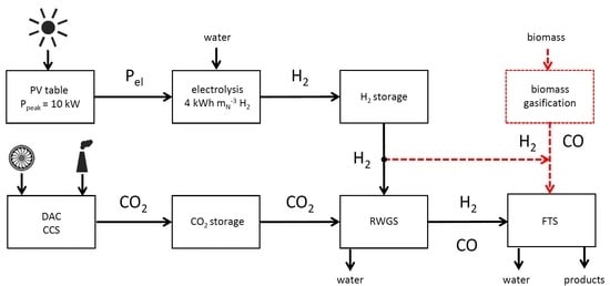
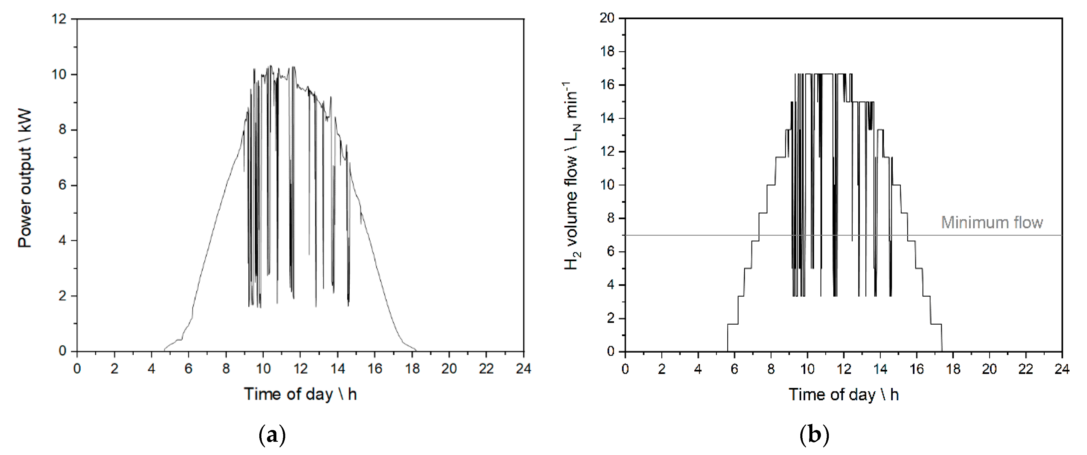
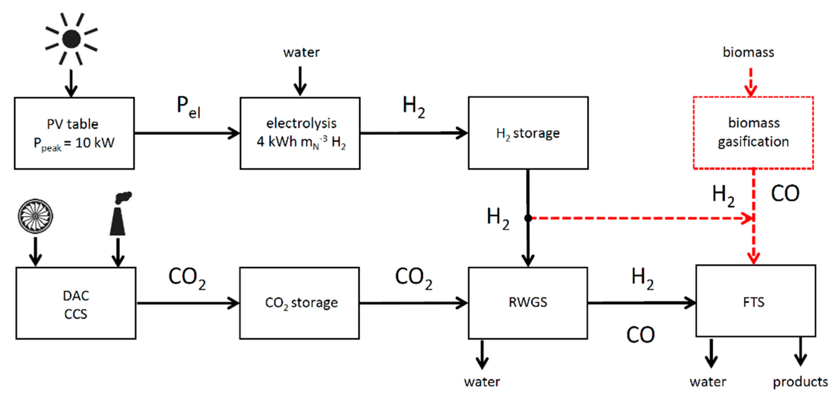
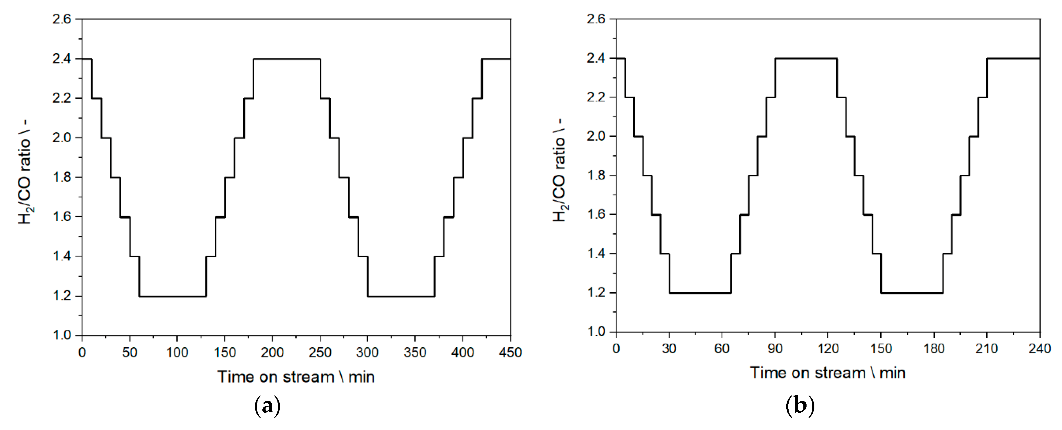
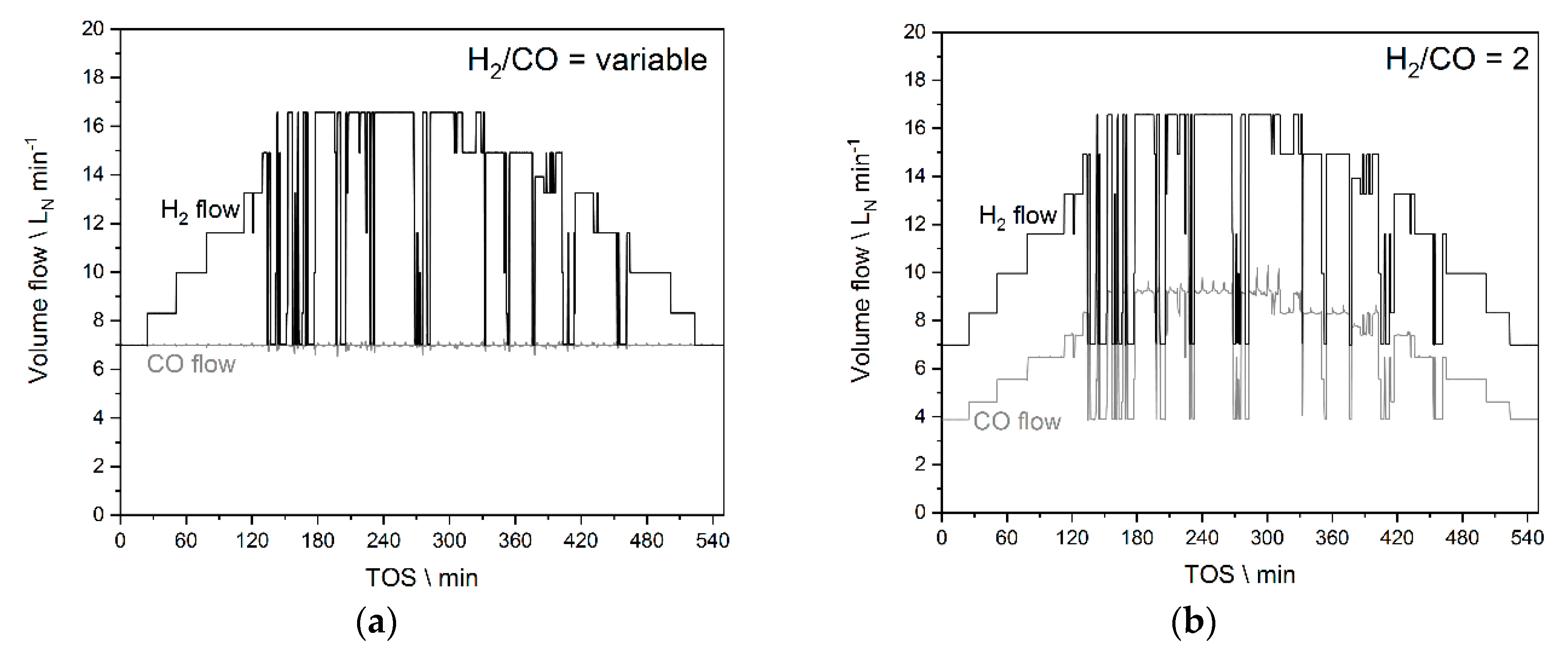
2.2. Real Photovoltaic Profiles and Discretization of the Feed

Since a realistic context of an actual PtL process is not yet fully clear, testing the capabilities of the FTS step is straightforward to identify possible limits of future process chains. Stress on the catalyst can be applied in many ways. In the context of dynamic FTS, quickly fluctuating feeds are a good way to test system behavior under extreme conditions.

KIT’s Battery Technical Center (BATEC) supplied different real-time profiles for a 10 kW photovoltaic (PV) table. This data was used to develop experimental campaigns. The PV table consists of polycrystalline solar modules. The tilt angle was adjusted to 30° facing south, which is considered optimal for the given location (N 49.1 E 8.4). This allowed reaching the theoretical peak power of 10 kW.

In this work, a daily profile for a sunny spring day in 2015 is used (see Figure 1a). It was confirmed by BATEC that this profile is a representative average for that period and location. A hydrogen flow of 4 kWh $m_{N,H_2}^{-3}$ was calculated from the assumption of a conversion efficiency of 75% (based on the heating value). This is a typical value for industrial state-of-the-art PEM electrolysis as reported for Siemens Silyzer 200 and 300 systems, for instance [41,42]. Usually, we operate the reactor in steady state between 60 and 160 g_cat h m⁻³ of syngas mixture (see Table 2). This equals between 5 and 17.6 L_N min⁻¹ of hydrogen. In order to achieve this, a downscaling factor of 2.5 was applied to fit the scale of H₂ production to the given reactor size and mass of catalyst. A discretization of the hydrogen volume flow was conducted to yield a maximum 10 steps during a ramp from the highest flow level to the lowest and vice versa. Furthermore, the time of a change between the different levels was expanded to minimum one minute so that new syngas flows could be established in the current test rig. A minimum flow of 7 L min⁻¹ H₂ needed to be guaranteed from experience in order to keep the specific pilot scale reactor running autothermal by emitting sufficient reaction enthalpy. This is crucial in order to compensate the losses to the environment and the cooling cycle. This is an experimental limitation in the current setup as a function of the reactor size and total mass of catalyst in the system. A scale-up factor of 60 would fortunately reduce this lower limit to less than 20% of the upper value, which allows a wider flexibility of the reaction. An additional 3 h of operation time per day (phases of dawn and twilight) would be feasible then without including a hydrogen storage.

The discretized input signal for the reaction is depicted in Figure 1b. After cutting the graph along the minimum flow, seven different experimental conditions remained.

2.3. Experimental Base Cases

In order to apply the hydrogen profile presented in Section 2.2, the two different scenarios were chosen to gather first insights into the process stability and product quality. Figure 2 shows the potential pathways for either PtL or BtL approaches including an FTS unit in a simplified scheme. For both cases, the abovementioned PV panel and electrolysis unit deliver the hydrogen needed for the FTS. The carbon source is either CO₂ or biomass.

For Case 1, the BtL pathway, a steady biomass gasification is assumed so that a constant flow of CO-rich synthesis gas is gathered with a syngas ratio below 2 [43]. If the fluctuating hydrogen flow from the electrolysis is added to the constant flow of synthesis gas, a varying H₂/CO ratio in the FTS reactor and changing residence time of the gas mixture are the consequences. Varying two system parameters at the same time promotes unpredictable effects on the performance of the synthesis.

In Case 2, the PtL process route, a CO₂ storage can be depleted on demand. It is assumed that a RWGS unit can be operated with fixed gas mixtures and changing total flows In-line with the response time of the electrolysis. In this scenario, a fixed H₂/CO ratio of 2 is fed to the FTS reactor. A dilution of the feed gas with CO₂ or formed methane of the RWGS output is not considered in the current approach. Water is thought to be condensed before entering the FTS.

2.4. Calculation of Conversion Levels during Quick Process Changes

The actual CO conversion could not be determined in real time since both GC and MS analysis suffer from product back mixing with at least 17.5 min of signal delay, see part 1 of the study [38]. In order to approximate conversion levels during quick changes, a linear regression model was developed, based on a database of 19 sets of process parameters that were tested experimentally. Parameter ranges are listed in

Table 1. Overview of process parameters for linear regression data in a pilot scale FTS unit

	Temperature °C	Syngas ratio -	τmod gcat h m−3
Min. value	235.5	1.49	65.17
Max. value	246	2.20	158.02

. Within these ranges, conversion estimations should be accurate.

The modified residence time (τ_mod), the syngas ratio and the temperature have a significant influence on CO conversion. Because of different gas densities between all gas feed species, the density-independent parameter τ_mod was chosen instead of the weight hourly space velocity (WHSV) and calculated via the relation τ_mod = γ_feed WHSV⁻¹ with γ_feed being the respective density of the feed gas mixture.

The correlation of CO conversion from the individual values can be described with a linear regression model. The fundamental approach is described in Equation (1). The regression coefficients β_k are linearly related.

$$X_{CO}={\beta }_0+{\beta }_1 x_1+{\beta }_2 x_2+\cdots +{\beta }_k x_k,$$

(1)

with X_CO being the CO conversion, ${\beta }_0$ the base regression coefficient, ${\beta }_k$ regression coefficients and $x_k$ regression variables. The regression coefficients weigh the expected change in X_CO with changes in regression variables. The variables for this model are combinations of the modified residence time, the H₂/CO ratio and the temperature. The model was fitted using a systematic approach based on Equation 1 executed in a standard spreadsheet calculator program. A linear approach according to Equation (2) was chosen [44].

$$X_{CO}={\beta }_0+{\beta }_1 X_{{\tau }_{mod}}+{\beta }_2 X_{\frac{H_2}{CO}}+{\beta }_3 X_{T_{Reactor}},$$

(2)

with X_i being the coefficients for the respective influence parameters mentioned above. T_Reactor is the average temperature determined from two thermocouples in the foil stack next. These are placed along the bed length in the outer wall of the catalyst bed. The individual parameters from Equation (2) can be determined using the least squares method. In matrix notation, the measured values can be specified as shown in Equation (3).

$$\overrightarrow{x}=\mathrm{H} · \overrightarrow{y},$$

(3)

with $\overrightarrow{x}$ being the results matrix, H the matrix notation of the target equation and $\overrightarrow{y}$ the estimator and the coefficient matrix. The variables are defined in Equation (4)

$$\overrightarrow{x}=\left(\begin{array}{c}{X}_{CO,1}\\ X_{CO,2}\\ ⋮\\ X_{CO,k}\end{array}\right)H=\left(\begin{array}{c}1\\ 1\\ ⋮\\ 1\end{array} \begin{array}{c}{X}_{{\tau }_{mod},1}\\ X_{{\tau }_{mod},2}\\ ⋮\\ X_{{\tau }_{mod},k}\end{array} \begin{array}{c}{X}_{\frac{H_2}{CO},1}\\ X_{\frac{H_2}{CO},2}\\ ⋮\\ X_{\frac{H_2}{CO},k}\end{array} \begin{array}{c}{X}_{T_{Reactor},1}\\ X_{T_{Reactor},2}\\ ⋮\\ X_{T_{Reactor,}k}\end{array}\right) \overrightarrow{y}=\left(\begin{array}{c}{\beta }_1\\ {\beta }_2\\ ⋮\\ {\beta }_k\end{array}\right),$$

(4)

For the estimator of the least squares method $\overrightarrow{y}$, the relation in Equation (5) can be used [45]

$$\overrightarrow{y}={\left({\mathrm{H}}^{\mathrm{T}}\mathrm{H}\right)}^{·1}{\mathrm{H}}^{\mathrm{T}}· \overrightarrow{x},$$

(5)

while matrix H must be of full rank for the inverse ${\left({\mathrm{H}}^{\mathrm{T}}\mathrm{H}\right)}^{-1}$ to exist. The residuals vector $\overrightarrow{e}$ can be determined from Equation (6)

$$\overrightarrow{e}=\overrightarrow{x}-\mathrm{H}· \overrightarrow{y}.$$

(6)

2.5. Step Change Experiments—Experimental Design

In order to test the system before PV profile experiments, step change experiments were conducted based on the seven remaining steps between minimum and maximum hydrogen flow, see Section 2.2. Reactor behavior was tested in accordance to Case 1 by manipulating the syngas ratio concurrently with the residence time of each step change. This was applied by giving a constant CO flow of 7 L_N min⁻¹, adding as much hydrogen as needed to reach certain H₂/CO ratios. The syngas ratio ranged consequently between 1.2 (very low) and 2.4 (over-stoichiometric) with 0.2-steps. The time between each step differed, starting with 10 min between each step (experiment A) to 5 min between each step (experiment B). A lower step time was unfavorable for the means of process observation since liquid sampling took 5 min. The initial syngas ratio was held overnight before each experiment. Two plateaus at minimum and maximum ratio were held for a prolonged time (60 min for experiment A, 30 min for experiment B) before ramping up or down again. Figure 3 shows the executed experiments.

2.6. Experiments Based on the PV Profile

For the PV profile experiments, the BtL and the PtL case was covered experimentally. Figure 4 shows the FTS feed input data with regard to H₂ and CO flow adapted from the real PV profile. Figure 4a represents Case 1 (experiment C) and Figure 4b Case 2; Case 1 was conducted with a larger range of the syngas ratio (1.0–2.4) compared to the step change experiments. Case 2 was first conducted without external temperature control (experiment D) and repeated. The linear regression model introduced in Section 2.4 was used to calculate the necessary temperature, which is required to keep the CO conversion throughout the experiment (experiment E). The aim was to convert 70% of CO despite the changing residence time inside the reactor. Therefore, temperature data from experiment D was analyzed and temperature corrections applied by hand if the conversion was below 70%.

3. Results and Discussion

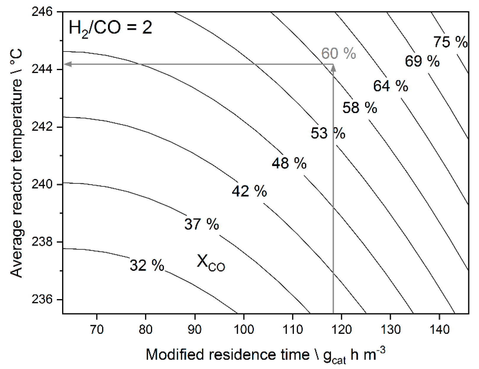
3.1. Linear Regression Model

Using the regression described in Section 2.4, the linear approach from Equation (2) was systematically adapted to 19 data points with low inert gas dilution (<5%) using the least squares method. For the fit, the data from

Table 2. Detailed overview of experimental data used for the linear regression model

Data	τmod gcat h m−3	H2/CO -	T °C	τnorm -	H2/COnorm -	Tnorm -	XCO %
1	93.91	1.98	245	0.3073	0.6855	0.9048	65.25
2	81.81	1.98	245	0.1779	0.6935	0.9048	55.72
3	72.74	2.11	244.5	0.0809	0.8757	0.8571	49.05
4	65.17	2.00	244.5	0.0000	0.7190	0.8571	41.58
5	65.27	2.00	235.5	0.0010	0.7214	0.0000	27.51
6	72.62	1.99	235.5	0.0797	0.7102	0.0000	27.61
7	81.74	1.99	235.5	0.1772	0.6993	0.0000	30.90
8	93.69	1.98	235.5	0.3050	0.6867	0.0000	36.06
9	158.02	1.94	235.5	0.9928	0.6295	0.0000	43.38
10	158.69	1.93	240	1.0000	0.6247	0.4286	57.79
11	141.32	1.49	244.5	0.8143	0.0000	0.8571	60.14
12	130.71	1.73	246	0.7008	0.3367	1.0000	62.14
13	121.26	1.96	244.5	0.5997	0.6593	0.8571	67.37
14	113.44	2.18	244.5	0.5161	0.9761	0.8571	71.34
15	94.22	2.19	241.5	0.3106	0.9875	0.5714	57.91
16	93.80	2.20	241	0.3061	0.9980	0.5238	42.37
17	94.69	2.20	240.5	0.3157	1.0000	0.4762	44.03
18	95.10	2.20	239	0.3200	0.9993	0.3333	43.29
19	107.33	1.96	238	0.4508	0.6658	0.2381	40.53

were used. Before the fit, the variables were normalized to a range between 0 and 1 using the min-max transformation according to Equation (7) [46]. This minimizes the influence of larger numbers on the regression.

$$x_{i,Norm}=\frac{x_i-x_{i,min}}{x_{i,max}-x_{i,min}}{x}_{i,Norm}ϵ\left[0,1\right],$$

(7)

with x_i being the respective value of the currently observed parameter, x_i,min being the lowest and x_i,max being the highest value of the parameter within the data set.

Equation (8) resulted from the linear regression for the measured data with a maximum deviation of 8.1%

$$X_{CO}=19.51+25.26 X_{{\tau }_{mod}}+13.20 X_{\frac{H_2}{CO}}+29.34 X_T.$$

(8)

Using Equation (8), the required reactor temperature was calculated depending on the feed conditions and the target CO conversion. The required reactor temperature to reach a certain CO conversion can be picked from a corresponding plot if τ_mod and the H₂/CO ratio are known. This tool was crucial for the planning of experiment E, where an increase in the conversion level based on the temperature should be achieved with quickly reducing residence times and vice versa. The contour plot based on Equation (8) is shown in Figure 5 for a fixed syngas ratio of 2 (Case 2). It was used to determine the conversion throughout experiment D and to calculate the needed temperature for 70% of CO conversion in experiment E.

The desired temperature was induced proactively by changing the water pressure used for evaporation cooling, see part 1 of our study [38].

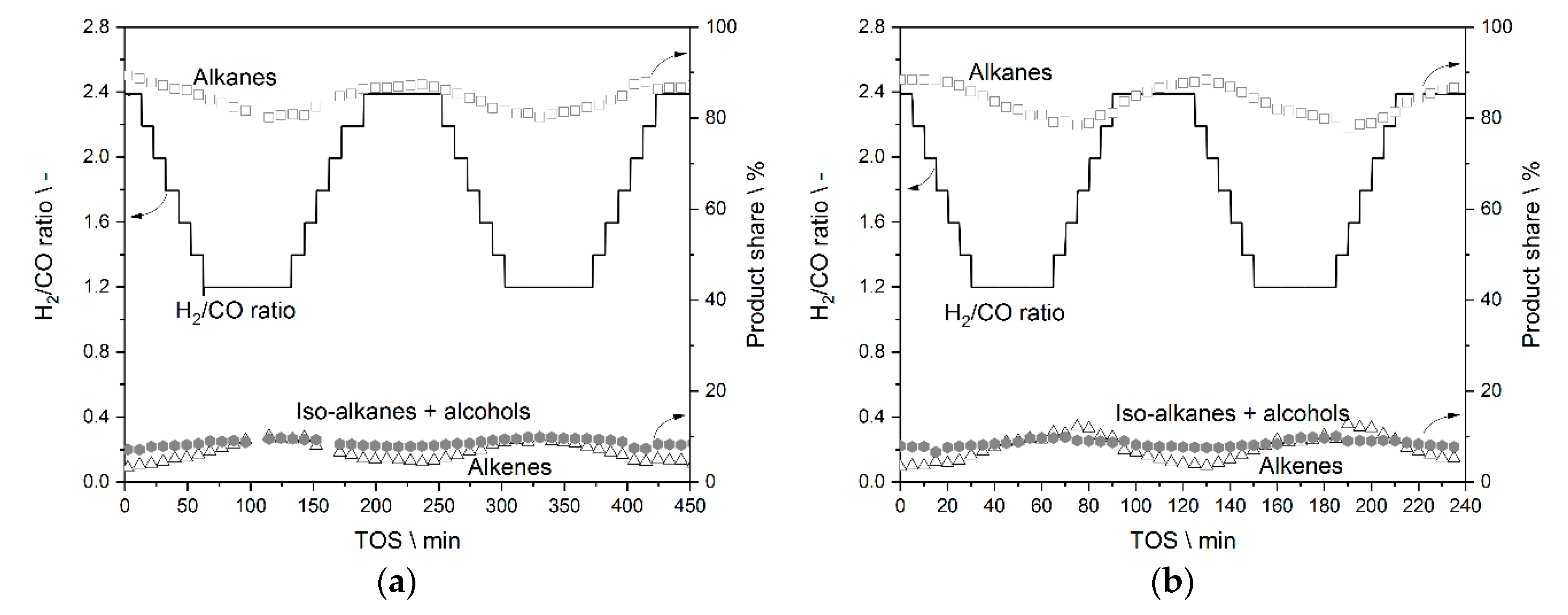
3.2. Step Change Experiments—Results

The outcome of the step change experiments is shown in Figure 6, Figure 7 and Figure 8. The average reactor temperature is shown in Figure 6a,b. The methane byproduct formation is depicted in Figure 7a,b and the composition of the liquid phase is represented by Figure 8a,b, for experiment A and B respectively. Temperature could be measured instantaneously at the reactor. Gas and liquid phase signals are delayed by a time shift of about 17.5 min compared to the moment when the gas concentration was changed, see part 1 of this work [38]. This shift is more apparent in the shorter time steps (Figure 7b and Figure 8b).

Figure 6a,b show the effect of different gas concentration change times on reaction temperature without external temperature control. The first plateau in experiment A led to a generally lower reactor temperature due to a longer time period at lower flow before the experiment. Thus, the slope of temperature increase in experiment B is consequently higher, leading to an increased maximum temperature after half of the experiment. Those effects could be countered by temperature manipulation, which was not conducted in these experiments.

A high syngas ratio strongly favors methane formation [47,48,49]. At higher temperatures, its formation is further increased, as Figure 7a,b show convincingly. The highest concentration gradient observed in both experiments was around Δc_CH4 = 10%_abs. Both experiments show quite similar concentration curves including similar delay of the methane signal. Some signal interruptions and relatively large signal noise are caused by the gas measurement via the Quick Sampling site which is frequently disconnected during liquid phase sampling, see part 1 of the study.

Figure 8a,b show the relative content of alkanes, alkenes and the sum of iso-alkanes and alcohols in the liquid phase. Saturation of molecules with hydrogen is dependent on the applied syngas ratio [50] and is visible as a shift between the alkanes’ and alkenes’ share in the experiments. The amounts of iso-alkanes and alcohols are quite constant despite significant changes of residence time and syngas ratio. The share is not influenced by temperature, as observed previously [38]. The progression of the curves is again similar for both time scales.

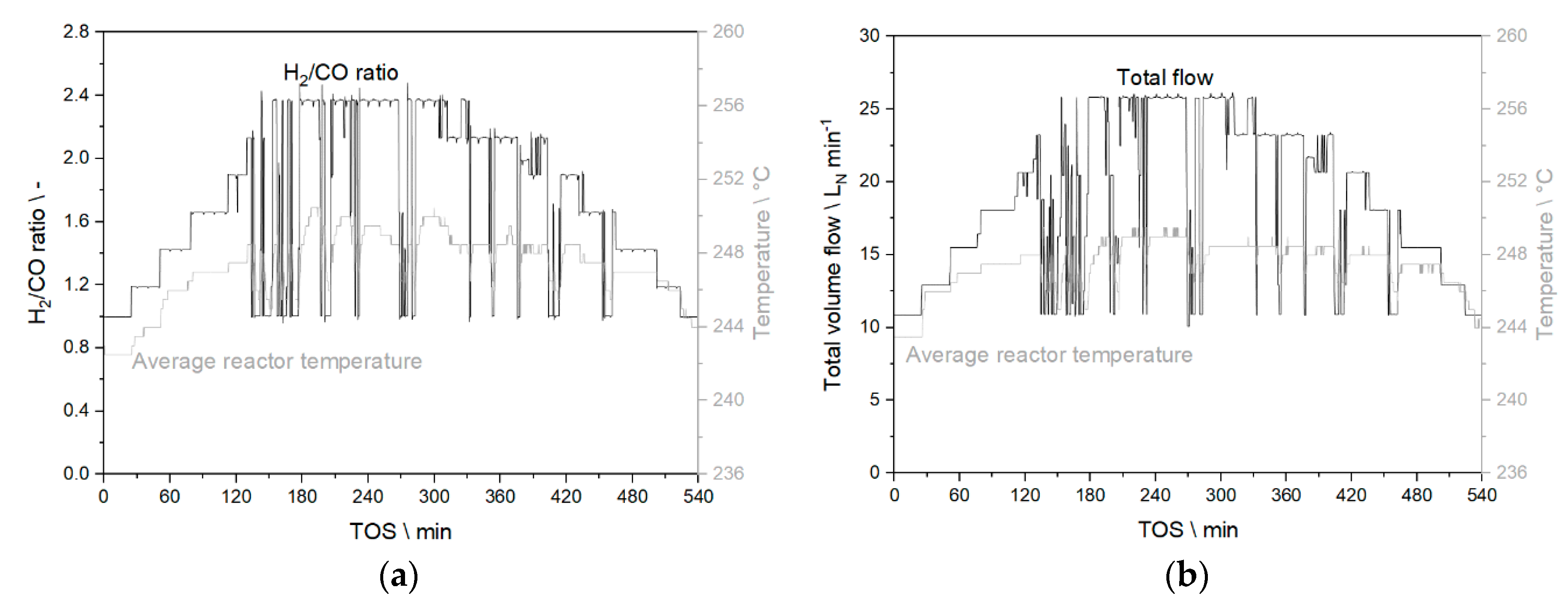
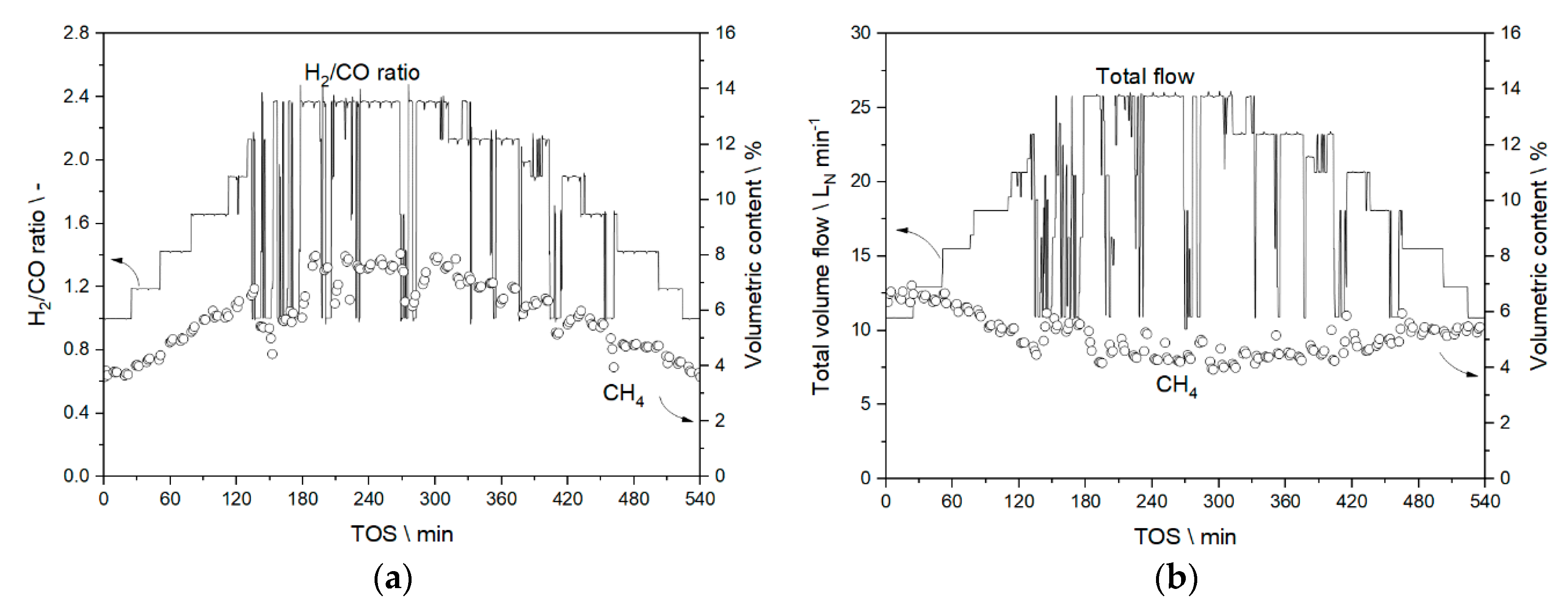
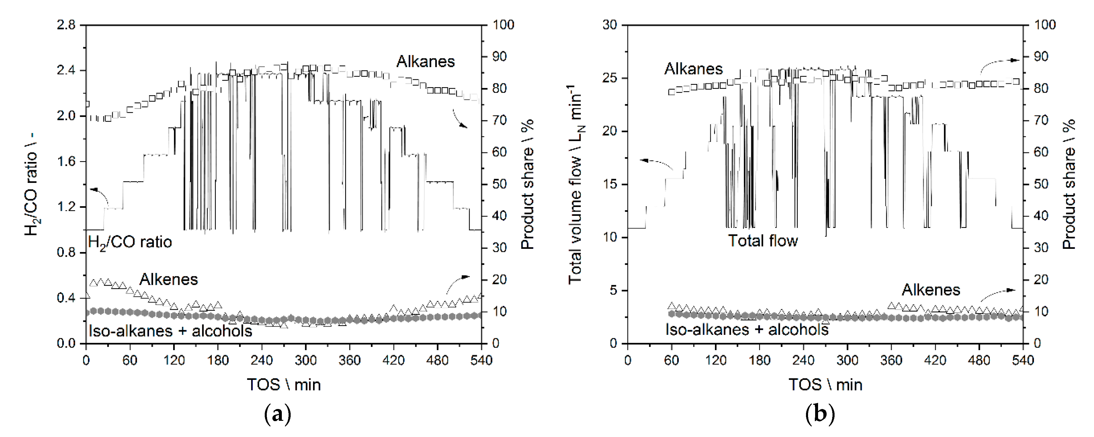
3.3. Experiments Based on the PV Profile—Results

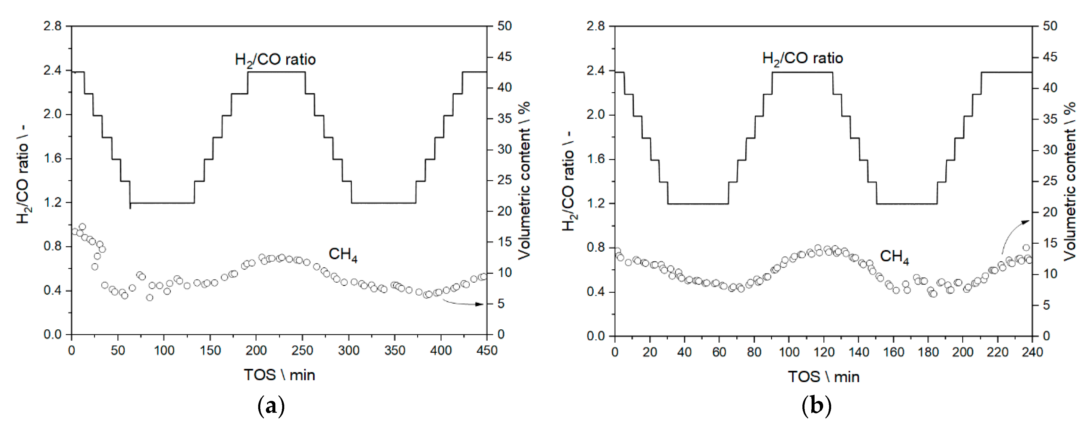
3.3.1. Results from Experiments without Temperature Manipulation

Experiment C is directly linked to the step change experiments as all are conducted with a constant CO flow. This, as explained earlier, simulates a BtL route without hydrogen buffer. Case 2 represents a PtL application without temperature manipulation (experiment D). Here, the existence of a CO₂ buffer storage is assumed as prerequisite for a dynamic operation of syngas production and utilization. Figure 9, Figure 10 and Figure 11 show the data on temperature, methane concentration, and liquid product composition in analogy to Figure 6, Figure 7 and Figure 8.

The reactor temperature in Figure 9a for experiment C shows similar behavior to the trend observed in experiments A and B. The average temperature inside the reactor increases with the available total gas flow and the hydrogen to CO ratio. The maximum average temperature change of the reactor in experiment C over the course of the experiment was ΔT_max = 8 °C, which is similar to the observed temperature change in step change experiments, see Section 3.2. The reactor is thus able to buffer fast changes in the 1 min regime while varying the residence time and syngas ratio; this is also valid with regard to a negligible T-gradient along the bed during the experiment. The reactor continued to run autothermally, and the cooling medium was never overheated. Neither did a thermal runaway happen.

Case 2, experiment D, is shown in Figure 9b. The maximum temperature of the reactor change is smaller, i.e., ΔT_max = 6 °C. This indicates that the influence of the residence time on the local temperature is much greater than that of the syngas ratio. The pronounced changes in volume flow can be counteracted by temperature manipulation, see next section. Regarding back-mixing of the products before the measurement unit and the general limitations in analysis time, no quantification of conversion could be performed at this point. This emphasizes the need of a prediction model like the one presented in Section 3.1.

Methane production in experiment C also followed the behavior observed in step change experiments. Figure 10a demonstrates that a higher available syngas ratio and the increasing reactor temperature resulted in an increased production rate for methane. The highest concentration gradient accounted for Δc_CH4,max = 4.5%_abs, which is only half the value from the step change experiments. Short changes seem to reduce the methane byproduct formation. Methane concentration was more constant in experiment D, as shown in Figure 10b. Δc_CH4,max is 3.5%_abs. Interestingly, the methane concentration is the inverse of the concentration in experiment C. At a lower total volume flow, the residence time of the feed gas increases and with it the conversion levels. With a higher conversion, the content of CH₄ in the product gas increases accordingly. Keeping a steady syngas ratio has positive effects on uniform methane production.

Figure 11a shows that the liquid composition is significantly influenced by the available syngas ratio in the catalyst bed, compare experiments A and B with C. The variation of the product shares of alkanes and alkenes is distinctly wider in experiment C compared to experiment D (Figure 11b) with constant syngas ratio. The iso-alkane and alcohol production seem mostly unaffected by the drastic changes applied. Even product properties are crucial for downstream operations such as distillation and hydrotreating. Keeping a constant syngas ratio is thus recommended. Therefore, the PtL case is advantageous compared to hydrogen-boosted BtL with regard to product upgrade.

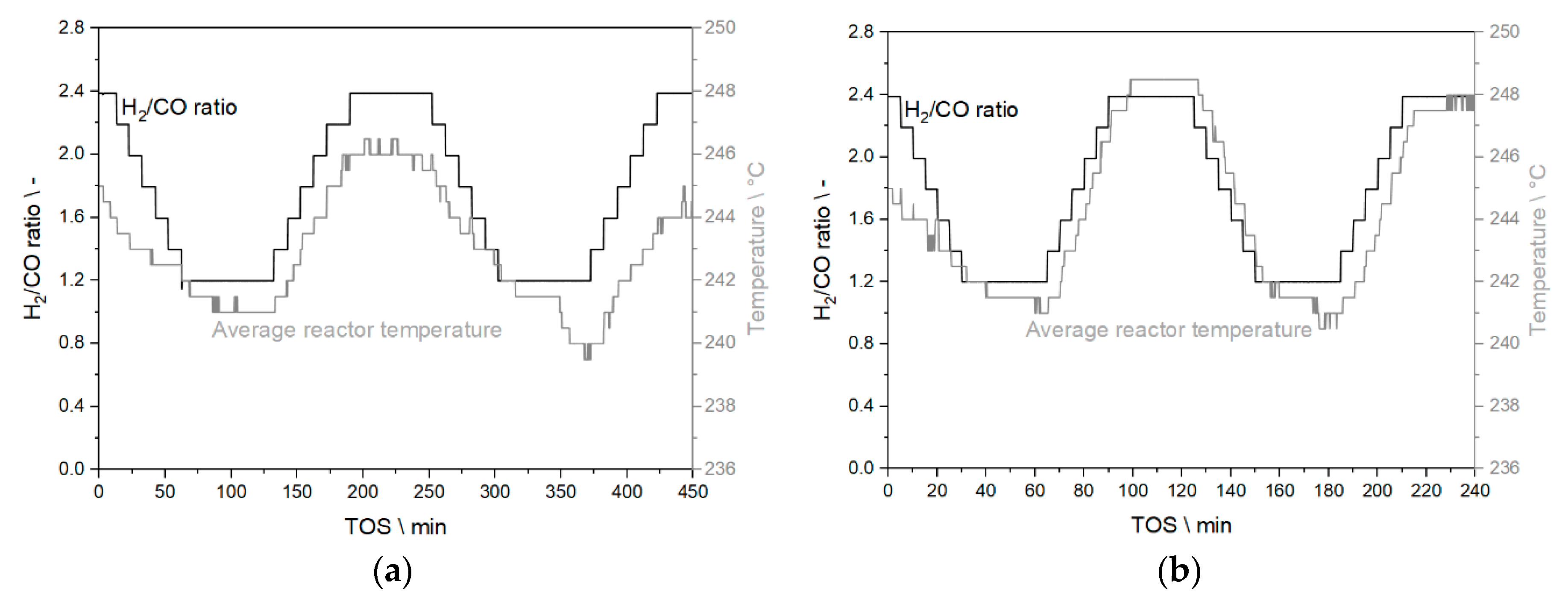
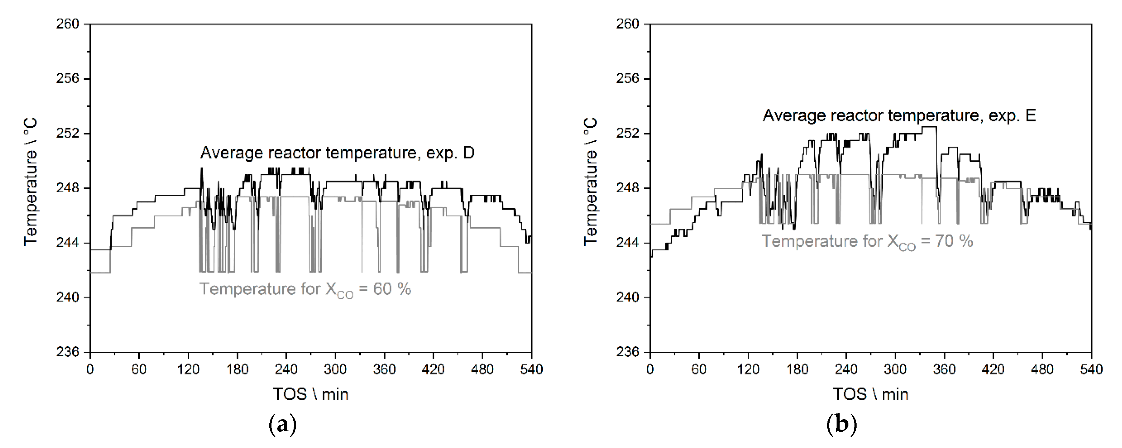
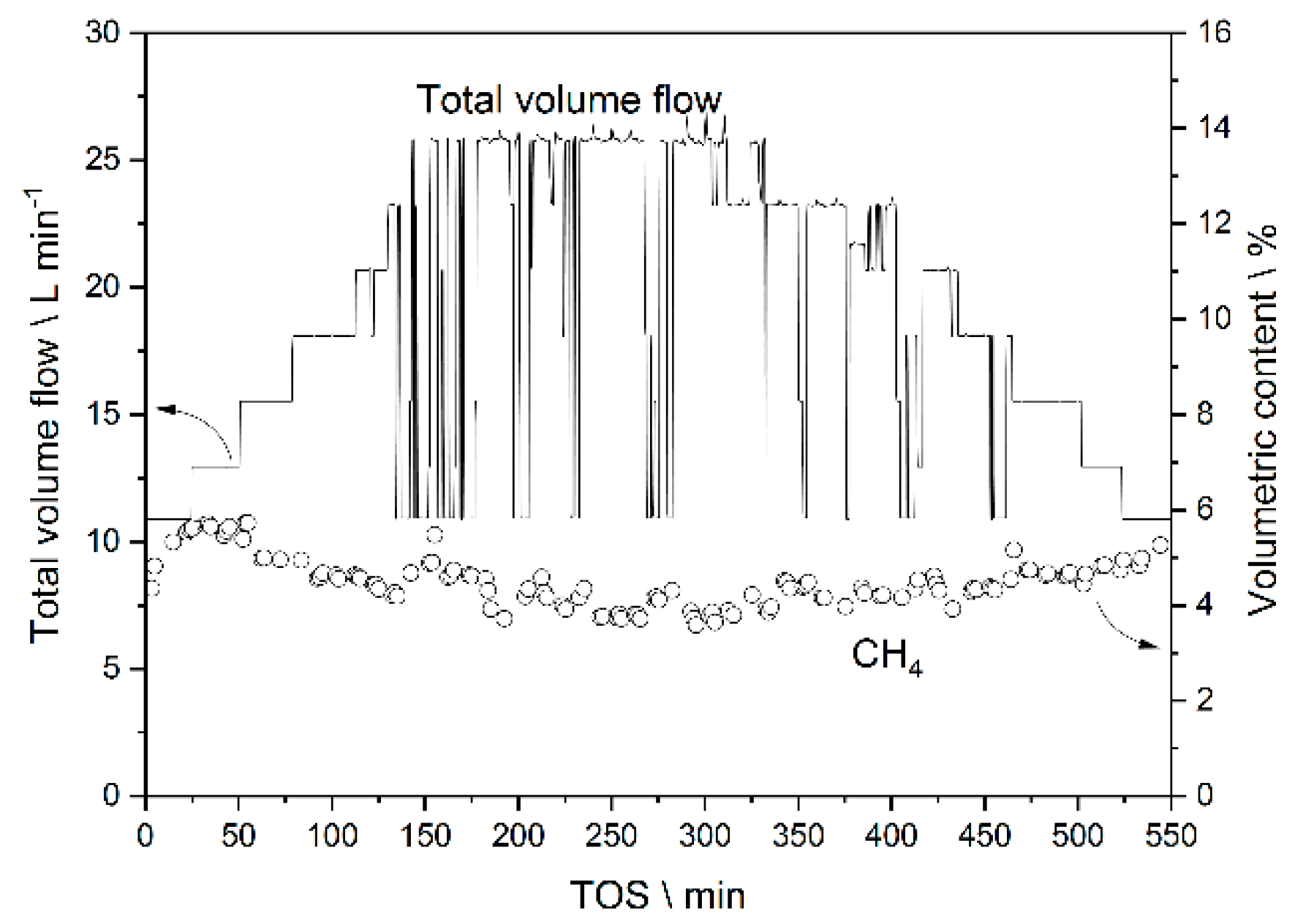
3.3.2. Results from Temperature Adaptation to Reach Targeted Conversion Levels

Experiment E also corresponds to the PtL route including a storage for CO₂ and a dynamically operated RWGS unit before the FTS. The reactor temperature is manipulated to aim for a CO conversion of 70+% at every time. The target temperature was calculated from the linear regression equation explained in Section 3.1. The required temperature setpoints as function of time were derived from the plot in Figure 9b as a base case and adapted by changing the water pressure in the cooling cycle per manual operation. The corresponding water pressure could be calculated with the Antoine equation for liquid water [51]. This manipulation was previously explored in part 1 of this study [38].

In Figure 12a, the required average reactor temperature for 60% CO conversion in experiment D is plotted against the measured value. Figure 12b shows the plot of required average reactor temperature for 70% CO conversion and the obtained average reactor temperature by manipulation of the cooling cycle pressure in experiment E. The upper plateau of the measured temperature is a consequence of reaching the evaporation state in the cooling cycle. Lower temperatures exist due to the effect that the reaction heat is not sufficient to reach the evaporation state and the reactor cools down due to heat loss to the environment. The reactor temperature could finally reach the setpoint of the water inlet temperature.

According to the linear regression model, experiment D without temperature manipulation already resulted in more than 60% CO conversion at any time during the experiment. Within experiment E, 70% of CO conversion should be reached at any time. It was possible to narrow the observed temperature profile and even to exceed the required temperature levels in some cases. The temperature was too low only during the first 120 min of the experiment. Starting at a low volume flow, the available reaction heat is limited, so less heat is available to increase the average temperature. Nevertheless, water pressure manipulation was in general an effective tool to reach high temperatures and thus high conversion. Above 75% conversion, the developed linear regression model leaves its validated parameter range so it is not possible to plot the conversion in the high temperature range obtained in experiment E.

With temperature control in experiment E, methane formation was even more uniform than in experiment D, see Figure 13. Δc_CH4,max was further decreased to 2.5%_abs. This highlights the superior performance of inherently temperature-flexible microstructured fixed bed reactors with regard to minimizing product deviations in dynamic load changes.

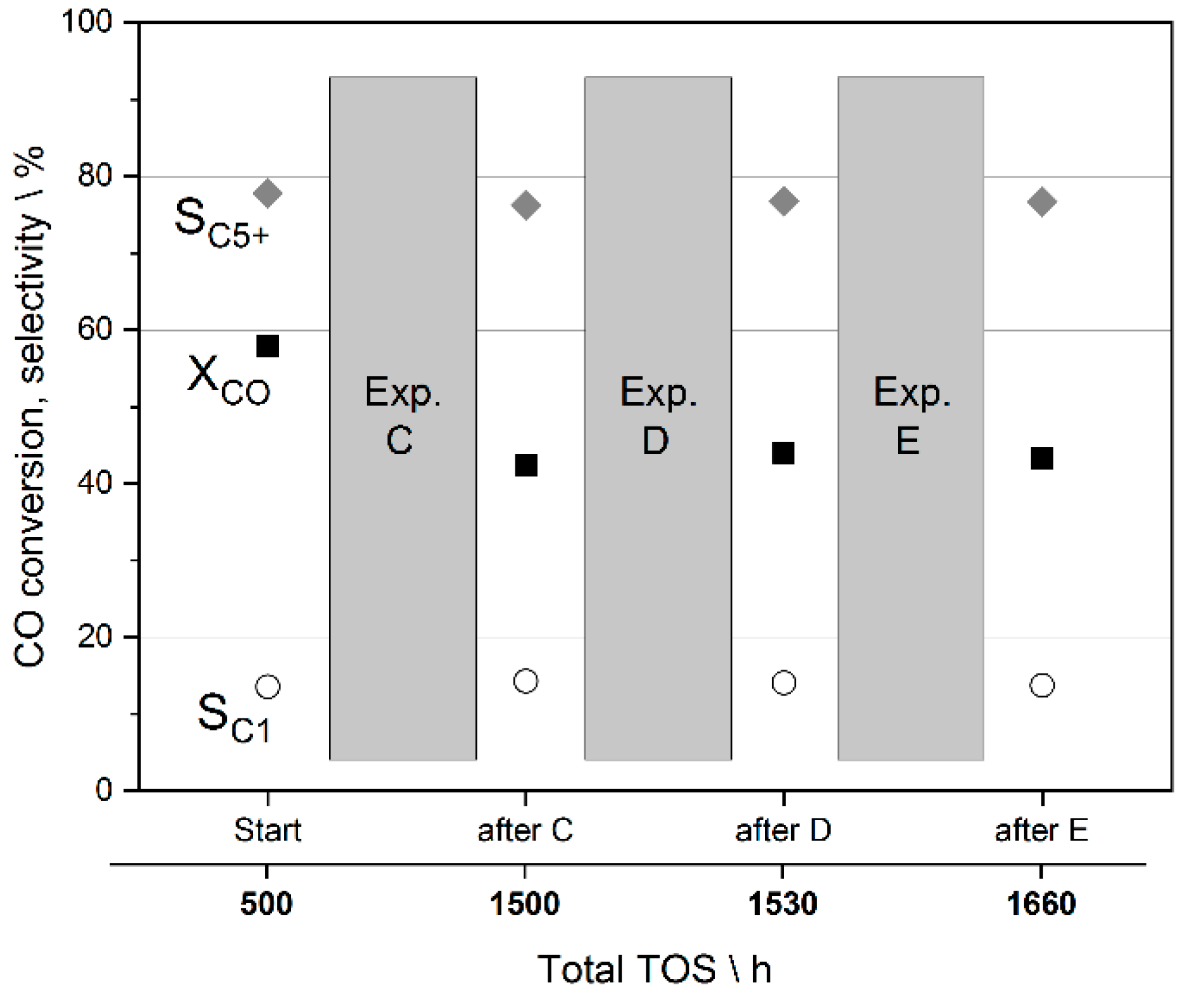
3.4. Preliminary Analysis of Effects on Catalyst Stability during the Studies

Long-term stability of the catalyst is crucial for any operation with economical interest. The effects from fluctuation in gas concentration and temperature on the FTS catalyst are yet unknown for most reactors, especially for microstructured reactors. The following analysis is preliminary as a continuous operation under load-flexible or dynamic conditions is to be performed on longer time scale.

Different criteria can be chosen to evaluate the state of the catalyst. Easiest to test is conversion and selectivity towards different product classes on a regular basis. This will not give sophisticated information on the state of the catalyst surface, specifically the active sites. In order to get a glimpse of surface effects, in-situ, or better, operando measurements are necessary. In the case of FTS, this is not a simple operation to perform. Process parameters like elevated pressure and temperature usually mean rough conditions for the equipment. Many reaction cells are designed to withstand the required temperature but are vulnerable to pressure. A complementary analysis of the metal surface and the reaction products allows for a more accurate interpretation of the observed phenomena. The methods of choice for operando analysis would be X-ray absorption (XAS) techniques, X-ray diffraction (XRD), and a coupled GC-MS analysis [19,52,53,54]. Those studies have been performed in an accompanied study and are subject of another publication under review [55].

In this work, catalyst activity was only evaluated by GC analysis. In Figure 14, the CO conversion and selectivity towards methane (S_C1) and liquid products (S_C5+) are shown. The same experimental condition was tested multiple times to determine the given values. The figure shows the respective value changes from data points 15–18 of Table 2 (identical parameters: H₂/CO = 2.2, ~240 °C, 30 bar_abs, 94.5 g_cat h m⁻³). Between the measurement of data point 15 (‘before experiments’) and setup 16 (‘after experiment C’), around 1000 h of operation elapsed, during which many different other data were collected from the reactor. In order to isolate the effect of the dynamic cycles on the catalyst from those trials, this data point should have been assessed right before experiment C. However, since this test was not executed, it is difficult to formulate a final assumption on when the catalyst actually deactivated.

Nevertheless, the CO conversion drop from around 58% to 42.4% within 1000 h of TOS may be correlated much more to the TOS than to experiments A, B and C themselves. This is supported by further constant values for all following experiments (more experiments were conducted that are not the subject of this study). It thus may be concluded that experiment D and E had no effect on catalyst performance. Complementary measurements are, nevertheless, needed for final statements.

4. Conclusions

In part 2 of this study, the challenges of a fluctuating energy supply are tackled. Sector coupling via dynamic operation of a microstructured packed bed reactor for FTS according to step changes and a real PV profile are assumed. From this study, it may be concluded that storage of fluctuating energy on minute- to season-scale via generation of chemical compounds seems feasible with the applied micro-technology. This claim is supported by the superior load flexibility of microstructured reactors. Even though it seems that intermediate hydrogen buffering can be omitted to large extent, economic considerations need to be performed to provide the realistic scenario at which time-scale load flexibility is actually required. It is also unclear how long the catalyst system would persevere in such specific scenarios. From this study, it may be concluded that dynamic operation is feasible in microstructured reactors without considerable influence on degradation. System changes in that time-scale are only possible due to the previously described, increased heat and mass transfer within those reactors and the application of pressure changes via evaporation cooling.

Available PV data from KIT’s solar park were translated into time-resolved hydrogen or syngas flow assuming near instantaneous conversion by electrolysis and reverse water-gas shift. The data was discretized to adjust to manageable setpoint changes in a pilot FTS test rig. Two base cases were developed, on which further experiments were performed. Case 1: a small-scale BtL plant where hydrogen is co-fed according to the PV power availability without a hydrogen buffer, leading to feed flow and H₂/CO ratio fluctuations. Case 2: a PtL plant without hydrogen buffer but a CO₂ storage leading to only feed flow fluctuations. Some facts have been neglected, such as the product gas from the RWGS would always include a dilution by inert gases such as CH₄ or CO₂. Nevertheless, effects from high dilution on the catalyst were investigated before [18].

Initial step change experiments were carried out to test the discretized steps from which it could be concluded that the system can buffer simultaneous syngas ratio and residence time changes with regard to thermal behavior and product quality. No obvious changes were found when varying the timeframe of the steps. Experiments with PV data were executed without and with temperature manipulation to emphasize the importance of evaporation cooling as the main tool to even product quality with fluctuating feed. Case 1, the BtL case, yielded unfavorable higher concentration differences along the fluctuation. Case 2 (PtL) showed a much steadier performance, as demonstrated by plots of methane concentration, as well as alkane and alkene content of the liquid product as a function of time.

It could be proven that highly dynamic, load flexible operation in microstructured FT reactors with multi-parameter changes in the one-minute regime are feasible and fully controllable. No runaway or blowout was found during fast changes of experimental conditions. The development of a regression model for adapting the reactor temperature without the need for measuring the product composition—i.e., only on basis of the knowledge of syngas ratio and residence time—led to almost even product quality. Constant product quality is important for product post-processing such as distillation and hydrotreating and highlights the importance of such methods. Keeping the CO conversion level by temperature manipulation seems to be a suitable approach for PtL plants as determined in this study. With a fixed H₂/CO ratio, reaching the goal of a target conversion of 70% by temperature manipulation via the pressure in the evaporating cooling cycle was experimentally verified as good strategy.

Due to the fact of relatively small total flows in the pilot scale FTS test rig, it was difficult to increase system temperature on demand from all starting points. This observation would improve with larger reactors. Consequently, autothermal operation will be possible with even lower relative loads, leading to more hours of operation without considerable hydrogen storage.

Changes in the test rig were done manually, which can be optimized. Last but not least, no apparent signs of catalyst damage were found through dynamic experiments. Nevertheless, operando technology would enable a deeper look onto the catalyst’s active sites to determine if the applied process caused negative effects on long-term activity.

References

1. UN Climate Change. Historic Paris Agreement on Climate Change: 195 Nations Set Path to Keep Temperature Rise Well Below 2 Degrees Celsius. Available online: http://newsroom.unfccc.int/unfccc-newsroom/finale-cop21/ (accessed on 3 April 2018).
2. BMU. Hendricks startet Dialog zum Klimaschutzplan 2050. Available online: https://www.bmu.de/pressemitteilung/hendricks-startet-dialog-zum-klimaschutzplan-2050/?tx_ttnews%5BbackPid%5D=3915 (accessed on 12 February 2020).
3. Le Quéré, C.; Andrew, R.M.; Friedlingstein, P.; Sitch, S.; Hauck, J.; Pongratz, J.; Pickers, P.A.; Korsbakken, J.I.; Peters, G.P.; Canadell, J.G.; et al. Global Carbon Budget 2018. Earth. Syst. Sci. Data 2018, 10, 2141–2194. [Google Scholar] [CrossRef] [Green Version]
4. Dittmeyer, R.; Boeltken, T.; Piermartini, P.; Selinsek, M.; Loewert, M.; Dallmann, F.; Kreuder, H.; Cholewa, M.; Wunsch, A.; Belimov, M.; et al. Micro and micro membrane reactors for advanced applications in chemical energy conversion. Curr. Opin. Chem. Eng. 2017, 17, 108–125. [Google Scholar] [CrossRef]
5. Maitlis, P.M.; de Klerk, A. (Eds.) Greener Fischer–Tropsch Processes for Fuels and Feedstocks; Wiley-VCH: Weinheim, Germany, 2013; ISBN 3527329455. [Google Scholar]
6. Verein Deutscher Ingenieure (VDI). VDI-Statusreport Regenerative Energien. Available online: https://www.vdi.de/ueber-uns/presse/publikationen/details/vdi-statusreport-regenerative-energien (accessed on 11 April 2020).
7. SAPEA—Science Advice for Policy by European Academies. Novel Carbon Capture and Utilisation Technologies. Available online: https://www.sapea.info/wp-content/uploads/CCU-report-web-version.pdf (accessed on 11 April 2020).
8. International Energy Agency (IEA). World Energy Outlook 2016. Available online: https://webstore.iea.org/world-energy-outlook-2016 (accessed on 11 April 2020).
9. Vaillancourt, K.; Bahn, O.; Roy, P.O.; Patreau, V. Is there a future for new hydrocarbon projects in a decarbonizing energy system? A case study for Quebec (Canada). Appl. Energy 2018, 218, 114–130. [Google Scholar] [CrossRef]
10. Ridjan, I.; Mathiesen, B.V.; Connolly, D. Terminology used for renewable liquid and gaseous fuels based on the conversion of electricity: A review. J. Clean. Prod. 2016, 112, 3709–3720. [Google Scholar] [CrossRef]
11. Li, W.; Wang, H.; Jiang, X.; Zhu, J.; Liu, Z.; Guo, X.; Song, C. A short review of recent advances in CO2 hydrogenation to hydrocarbons over heterogeneous catalysts. RSC Adv. 2018, 8, 7651–7669. [Google Scholar] [CrossRef] [Green Version]
12. Reuß, M.; Grube, T.; Robinius, M.; Preuster, P.; Wasserscheid, P.; Stolten, D. Seasonal storage and alternative carriers: A flexible hydrogen supply chain model. Appl. Energy 2017, 200, 290–302. [Google Scholar] [CrossRef]
13. Kotzur, L.; Markewitz, P.; Robinius, M.; Stolten, D. Time series aggregation for energy system design: Modeling seasonal storage. Appl. Energy 2018, 213, 123–135. [Google Scholar] [CrossRef] [Green Version]
14. Schmidt, P.; Batteiger, V.; Roth, A.; Weindorf, W.; Raksha, T. Power-to-Liquids as Renewable Fuel Option for Aviation: A Review. Chem. Ing. Tech. 2018, 127–140. [Google Scholar] [CrossRef]
15. De Klerk, A. Fischer–Tropsch Refining, 1st ed.; Wiley-VCH: Weinheim, Germany, 2011; ISBN 3527326057. [Google Scholar]
16. Piermartini, P.; Boeltken, T.; Selinsek, M.; Pfeifer, P. Influence of channel geometry on Fischer–Tropsch synthesis in microstructured reactors. Chem. Eng. J. 2017, 313, 328–335. [Google Scholar] [CrossRef]
17. Myrstad, R.; Eri, S.; Pfeifer, P.; Rytter, E.; Holmen, A. Fischer–Tropsch synthesis in a microstructured reactor. Catal. Today 2009, 147, 301–304. [Google Scholar] [CrossRef]
18. Loewert, M.; Hoffmann, J.; Piermartini, P.; Selinsek, M.; Dittmeyer, R.; Pfeifer, P. Microstructured Fischer–Tropsch reactor scale-up and opportunities for decentralized application. Chem. Eng. Technol. 2019, 2202–2214. [Google Scholar] [CrossRef]
19. Kalz, K.F.; Kraehnert, R.; Dvoyashkin, M.; Dittmeyer, R.; Gläser, R.; Krewer, U.; Reuter, K.; Grunwaldt, J.D. Future Challenges in Heterogeneous Catalysis: Understanding Catalysts under Dynamic Reaction Conditions. ChemCatChem 2017, 9, 17–29. [Google Scholar] [CrossRef] [Green Version]
20. Silveston, P.; Hudgins, R.R.; Renken, A. Periodic operation of catalytic reactors-introduction and overview. Catal. Today 1995, 25, 91–112. [Google Scholar] [CrossRef] [Green Version]
21. Güttel, R. Study of Unsteady-State Operation of Methanation by Modeling and Simulation. Chem. Eng. Technol. 2013, 83. [Google Scholar] [CrossRef]
22. Iglesias González, M. Gaseous Hydrocarbon Synfuels from H2/CO2 based on Renewable Electricity Kinetics, Selectivity and Fundamentals of Fixed-Bed Reactor Design for Flexible Operation. Ph.D. Thesis, Karlsruhe Institute of Technology (KIT), Karlsruhe, Germany, 2016. [Google Scholar]
23. Iglesias González, M.; Schaub, G. Fischer–Tropsch synthesis with H2/CO2-catalyst behavior under transient conditions. Chem. Ing. Tech. 2015, 87, 848–854. [Google Scholar] [CrossRef]
24. Eilers, H.; González, M.I.; Schaub, G. Lab-scale experimental studies of Fischer–Tropsch kinetics in a three-phase slurry reactor under transient reaction conditions. Catal. Today 2015. [Google Scholar] [CrossRef]
25. Mutz, B.; Carvalho, H.W.P.; Mangold, S.; Kleist, W.; Grunwaldt, J.-D. Methanation of CO2: Structural response of a Ni-based catalyst under fluctuating reaction conditions unraveled by operando spectroscopy. J. Catal. 2015, 327, 48–53. [Google Scholar] [CrossRef]
26. Kreitz, B.; Wehinger, G.D.; Turek, T. Dynamic simulation of the CO2 methanation in a micro-structured fixed-bed reactor. Chem. Eng. Sci. 2019, 195, 541–552. [Google Scholar] [CrossRef]
27. Kreitz, B.; Friedland, J.; Güttel, R.; Wehinger, G.D.; Turek, T. Dynamic Methanation of CO2—Effect of Concentration Forcing. Chem. Ing. Tech. 2019, 91, 576–582. [Google Scholar] [CrossRef]
28. Fache, A.; Marias, F.; Guerré, V.; Palmade, S. Optimization of fixed-bed methanation reactors: Safe and efficient operation under transient and steady-state conditions. Chem. Eng. Sci. 2018, 192, 1124–1137. [Google Scholar] [CrossRef]
29. Tauer, G.; Kern, C.; Jess, A. Transient Effects during Dynamic Operation of a Wall-Cooled Fixed-Bed Reactor for CO2 Methanation. Chem. Eng. Technol. 2019, 42, 2401–2409. [Google Scholar] [CrossRef] [Green Version]
30. Theurich, S.; Rönsch, S.; Güttel, R. Transient Flow Rate Ramps for Methanation of Carbon Dioxide in an Adiabatic Fixed-Bed Recycle Reactor. Energy Technol. 2020, 8, 1901116. [Google Scholar] [CrossRef]
31. Bremer, J.; Sundmacher, K. Operation range extension via hot-spot control for catalytic CO2 methanation reactors. React. Chem. Eng. 2019, 4, 1019–1037. [Google Scholar] [CrossRef] [Green Version]
32. Fache, A.; Marias, F.; Guerré, V.; Palmade, S. Intermittent Operation of Fixed-Bed Methanation Reactors: A Simple Relation Between Start-Up Time and Idle State Duration. Waste Biomass Valoriz. 2020, 11, 447–463. [Google Scholar] [CrossRef]
33. Fache, A.; Marias, F.; Chaudret, B. Catalytic reactors for highly exothermic reactions: Steady-state stability enhancement by magnetic induction. Chem. Eng. J. 2020, 390, 124531. [Google Scholar] [CrossRef]
34. Fache, A.; Marias, F. Dynamic operation of fixed-bed methanation reactors: Yield control by catalyst dilution profile and magnetic induction. Renew. Energy 2020, 151, 865–886. [Google Scholar] [CrossRef]
35. Bremer, J.; Rätze, K.H.G.; Sundmacher, K. CO2 methanation: Optimal start-up control of a fixed-bed reactor for power-to-gas applications. AIChE J. 2017, 63, 23–31. [Google Scholar] [CrossRef] [Green Version]
36. Theurich, S. Unsteady-state operation of a fixed-bed recycle reactor for the methanation of carbon dioxide. Ph.D. Thesis, Ulm university, Ulm, Germany, 2019. [Google Scholar]
37. Adesina, A.A.; Silveston, P.L.; Hudgins, R.R. A Comparison of Forced Feed Cycling of the Fischer–Tropsch Synthesis over Iron and Cobalt Catalysts. In Catalysis on the Energy Scene; Elsevier: Amsterdam, Netherlands, 1984; pp. 191–196. ISBN 9780444424020. [Google Scholar]
38. Loewert, M.; Pfeifer, P. Dynamically Operated Fischer–Tropsch Synthesis in PtL-Part 1: System Response on Intermittent Feed. ChemEngineering 2020, 4, 21. [Google Scholar] [CrossRef] [Green Version]
39. Sun, C.; Zhan, T.; Pfeifer, P.; Dittmeyer, R. Influence of Fischer–Tropsch synthesis (FTS) and hydrocracking (HC) conditions on the product distribution of an integrated FTS-HC process. Chem. Eng. J. 2017, 310, 272–281. [Google Scholar] [CrossRef]
40. Sun, C.; Pfeifer, P.; Dittmeyer, R. One-stage syngas-to-fuel in a micro-structured reactor: Investigation of integration pattern and operating conditions on the selectivity and productivity of liquid fuels. Chem. Eng. J. 2017, 326, 37–46. [Google Scholar] [CrossRef]
41. Tremel, A. Electricity-Based Fuels; Springer International Publishing: Cham, Switzerland, 2018; ISBN 9783319724591. [Google Scholar]
42. SIEMENS. SILYZER 300-Die Nächste Dimension der PEM-Elektrolyse. Available online: https://assets.new.siemens.com/siemens/assets/api/uuid:abae9c1e48d6d239c06d88e565a25040ed2078dc/version:1524040818/ct-ree-18-047-db-silyzer-300-db-de-en-rz.pdf (accessed on 29 March 2020).
43. Monaco, F.; Lanzini, A.; Santarelli, M. Making synthetic fuels for the road transportation sector via solid oxide electrolysis and catalytic upgrade using recovered carbon dioxide and residual biomass. J. Clean. Prod. 2018, 170, 160–173. [Google Scholar] [CrossRef]
44. Montgomery, D.C. Design and Analysis of Experiments, 8th ed.; John Wiley & Sons Inc.: Hoboken, NJ, USA, 2013. [Google Scholar]
45. Stiller, C. Grundlagen der Mess-und Regelungstechnik; Shaker: Aachen, Germany, 2006; ISBN 3-8322-5582-6. [Google Scholar]
46. Mueller, J.P.; Massaron, L. Machine Learning for Dummies; John Wiley & Sons, Inc.: New York, NY, USA, 2016; ISBN 978-1-119-24551-3. [Google Scholar]
47. Todic, B.; Ma, W.; Jacobs, G.; Davis, B.H.; Bukur, D.B. Effect of process conditions on the product distribution of Fischer–Tropsch synthesis over a Re-promoted cobalt-alumina catalyst using a stirred tank slurry reactor. J. Catal. 2014, 311, 325–338. [Google Scholar] [CrossRef]
48. Van der Laan, G.P.; Beenackers, A.A.C.M. Kinetics and Selectivity of the Fischer–Tropsch Synthesis: A Literature Review. Catal. Rev. 1999, 41, 255–318. [Google Scholar] [CrossRef]
49. Yates, I.C.; Satterfield, C.N. Hydrocarbon selectivity from cobalt Fischer–Tropsch catalysts. Energy Fuels 1992, 6, 308–314. [Google Scholar] [CrossRef]
50. Dry, M.E. Practical and theoretical aspects of the catalytic Fischer–Tropsch process. Appl. Catal. A-Gen. 1996, 138, 319–344. [Google Scholar] [CrossRef]
51. VDI-Gesellschaft Verfahrenstechnik und Chemieingenieurwesen. VDI Heat Atlas, 2nd ed.; Springer: Heidelberg/Neckar, Germany, 2010; ISBN 9783540799993. [Google Scholar]
52. Rønning, M.; Tsakoumis, N.E.; Voronov, A.; Johnsen, R.E.; Norby, P.; van Beek, W.; Borg, Ø.; Rytter, E.; Holmen, A. Combined XRD and XANES studies of a Re-promoted Co/γ-Al2O3 catalyst at Fischer–Tropsch synthesis conditions. Catal. Today 2010, 155, 289–295. [Google Scholar] [CrossRef]
53. Grunwaldt, J.-D.; Clausen, B.S. Combining XRD and EXAFS with on-Line Catalytic Studies for in situ Characterization of Catalysts. Top. Catal. 2002, 18, 37–43. [Google Scholar] [CrossRef]
54. Rochet, A.; Moizan, V.; Pichon, C.; Diehl, F.; Berliet, A.; Briois, V. In situ and operando structural characterisation of a Fischer–Tropsch supported cobalt catalyst. Catal. Today 2011, 171, 186–191. [Google Scholar] [CrossRef]
55. Loewert, M.; Serrer, M.-A.; Carambia, T.; Stehle, M.; Zimina, A.; Kalz, K.F.; Lichtenberg, H.; Saraci, E.; Pfeifer, P.; Grunwaldt, J.-D. Bridging the gap between industry and synchrotron: An operando study at 30 bar over 300 h during Fischer–Tropsch synthesis. React. Chem. Eng. 2020. [Google Scholar] [CrossRef] [Green Version]
Figure 1. Experimental input signals based on the data from KIT’s Battery Technical Center (BATEC). (a) Power output profile for a 10 kW peak PV table for a sunny spring day in 2015; (b) Discretized hydrogen flow calculated from Figure 1a assuming a specific conversion energy of 4 kWh m N , H 2 3 and applying a further downscaling factor of 2.5.
Chemengineering 04 00027 g001
Figure 2. Potential PtL (black solid lines) and BtL (red dotted lines) pathways to produce syngas for the microstructured FTS reactor. Both pathways include a PV panel and electrolyzer; a hydrogen buffer storage of a certain size is optional. The PtL pathway utilizes CO2 as carbon source exclusively, which needs to be converted into syngas in a RWGS unit. A CO2 buffer storage is an assumed pre-requisite here. The BtL pathway uses syngas from biomass gasification and hydrogen from electrolysis.
Chemengineering 04 00027 g002
Figure 3. Setpoints of H2/CO ratio between 1.2 and 2.4 with two cycles of ramping it down and up as function of time in step change experiments. (a) Experimental profile for ten-minute steps with plateau times of 60 min (experiment A); (b) Experimental profile for five-minute steps with plateau times of 30 min (experiment B).
Chemengineering 04 00027 g003
Figure 4. Setpoints of CO an H2 flow discretized from the PV profile as function of time. (a) Variable H2/CO ratio and residence time (Case 1, experiment C); (b) Variable residence time with a fixed syngas ratio of 2 (Case 2, valid for experiments D and E).
Chemengineering 04 00027 g004
Figure 5. Contour plot derived from Equation (8) with curves of constant CO conversion levels ranging from 32–75% as function of τmod and the average reactor temperature at a syngas ratio of 2.
Chemengineering 04 00027 g005
Figure 6. Average reactor temperature as function of time in step change experiments A (a) and B (b).
Chemengineering 04 00027 g006
Figure 7. Methane concentration as function of the time in step change experiments A (a) and B (b).
Chemengineering 04 00027 g007
Figure 8. Liquid phase composition regarding alkanes, alkenes and sum of iso-alkanes and alcohols in step change experiments A (a) and B (b).
Chemengineering 04 00027 g008
Figure 9. Average reactor temperature as function of time for experiments C (a) and D (b), the latter with a constant syngas ratio of 2.
Chemengineering 04 00027 g009
Figure 10. Methane concentration as function of time for experiments C (a) and D (b), the latter with a constant syngas ratio of 2.
Chemengineering 04 00027 g010
Figure 11. Liquid phase composition regarding alkanes, alkenes and the sum of iso-alkanes and alcohols as function of time for experiments C (a) and D (b), the latter with a constant syngas ratio of 2.
Chemengineering 04 00027 g011
Figure 12. Required average reactor temperature by linear regression to reach a certain conversion (grey solid line) and measured average reactor temperature (black solid line) as function of time. (a) experiment D with aimed 60% CO conversion; (b) experiment E with aimed 70% CO conversion.
Chemengineering 04 00027 g012
Figure 13. Methane concentration as function of time in the course of experiment E where the total applied feed flow was varied with a constant H2/CO ratio of 2 and concurrent temperature manipulation.
Chemengineering 04 00027 g013
Figure 14. CO conversion and selectivity towards methane (SC1) and liquid products (SC5+) over total experimental TOS. Four setups (15–18 from Table 2) are represented for the sake of activity measurement. Grey rectangles mark the experimental campaigns presented in this work (experiments C–E).
Chemengineering 04 00027 g014