Review

Multiscale Eulerian CFD of Chemical Processes: A Review

Center of Sustainable Process Engineering (CoSPE), Department of Chemical Engineering, Hankyong National University, Jungang-ro 327, Anseong-si 17579, Korea
*
Author to whom correspondence should be addressed.
ChemEngineering 2020, 4(2), 23; https://doi.org/10.3390/chemengineering4020023
Submission received: 8 February 2020 / Revised: 23 March 2020 / Accepted: 30 March 2020 / Published: 31 March 2020
(This article belongs to the Special Issue Computational Fluid Dynamics (CFD) of Chemical Processes)

Abstract

:
This review covers the scope of multiscale computational fluid dynamics (CFD), laying the framework for studying hydrodynamics with and without chemical reactions in single and multiple phases regarded as continuum fluids. The molecular, coarse-grained particle, and meso-scale dynamics at the individual scale are excluded in this review. Scoping single-scale Eulerian CFD approaches, the necessity of multiscale CFD is highlighted. First, the Eulerian CFD theory, including the governing and turbulence equations, is described for single and multiple phases. The Reynolds-averaged Navier–Stokes (RANS)-based turbulence model such as the standard k-ε equation is briefly presented, which is commonly used for industrial flow conditions. Following the general CFD theories based on the first-principle laws, a multiscale CFD strategy interacting between micro- and macroscale domains is introduced. Next, the applications of single-scale CFD are presented for chemical and biological processes such as gas distributors, combustors, gas storage tanks, bioreactors, fuel cells, random- and structured-packing columns, gas-liquid bubble columns, and gas-solid and gas-liquid-solid fluidized beds. Several multiscale simulations coupled with Eulerian CFD are reported, focusing on the coupling strategy between two scales. Finally, challenges to multiscale CFD simulations are discussed. The need for experimental validation of CFD results is also presented to lay the groundwork for digital twins supported by CFD. This review culminates in conclusions and perspectives of multiscale CFD.

1. Introduction

Many scientific problems have intrinsically multiscale nature [1,2]. This multiscale nature often leads to multiple spatial and temporal scales that cross the boundaries of continuum and molecular levels [3]. Multiscale simulations cover quantum mechanics, molecular dynamics (MD), coarse-grained particle dynamics, and continuum mechanics [4,5]. Multiscale modeling in science and engineering couples several methods that produce the best predictions at each scale [6], which can then be applied to materials engineering [7], computational chemistry [8], systems biology [9,10], molecular biology [11], drug delivery [12], semiconductor manufacturing [13], reaction engineering [14], fluid flow [5,15], and process engineering [2,16,17].
Multiscale modeling has been used in the form of sequential and concurrent couplings [4,15]. In a sequential coupling framework, often referred to as parameter passing between scales, the macroscale model uses a small number of parameters calculated in the microscale model. The concurrent coupling strategy computes several scale models simultaneously [1,4,16]. Concurrent coupling is preferred over sequential coupling when the missing information is a function of many variables. Concurrent coupling is a powerful approach but it is also computationally prohibitive [1].
Delgado-Buscalioni et al. (2005) presented a multiscale hybrid scheme coupling MD in a subdomain with computational fluid dynamics (CFD) in a continuum fluid domain [1]. Nanofluids typically employed as heat transfer fluids include multiphysics such as drag and lift forces between liquid and nanoparticles and Brownian, thermophoretic, van der Waals, and electrostatic double-layer forces [18]. Challenge remains in nanofluid flow simulations using a CFD model that includes multiphysics and a multiscale CFD model. Tong et al. (2019) reviewed multiscale methods divided into a domain decomposition scheme and a hierarchical scheme in fluid flows with heat transfer for coupling MD with particle-based mesoscale methods such as the lattice Boltzmann method (LBM) and CFD [15]. LBM using the particle distribution function is suitable for simulating fluid flows involving interfacial dynamics and complex boundaries [15,19]. The fundamental idea of LBM is that the macroscopic dynamics of a fluid are the result of the collective behavior of many microscopic particles in the system [19]. Thus, by integrating the particle momentum space, the particle distribution function (Boltzmann transport equation) at the microscopic scale is linked to the continuous fluid dynamic properties such as density, velocity, and energy at the macroscopic scale [3,20]. LBM is an alternative approach in CFD, which has been applied to fluid flows in porous media, microfluidics, and particulate flows [19,20]. However, because CFD based on LBM focuses on the microscopic domain with complex boundary conditions, macroscopic Eulerian CFD is preferred for investigating hydrodynamics on the process level [2,15].
Lagrangian CFD approaches such as the discrete element method (DEM) and the discrete phase model (DPM) solves the Newton’s second law of motion for each particle to identify the trajectories of the particles. The Lagrangian model is normally limited to a relatively small number of particles (less than 105 particles) because of the computational expense [17,21]. This review focuses on the Eulerian CFD for the continuum phase in chemical processes, excluding the more sophisticated methods such as the LBM and Lagrangian approaches.
Eulerian CFD has become a powerful and important tool for simulating and predicting fluid behaviors in chemical and biological processes [22]. Eulerian CFD provides the average quantities at the equipment-scale that are of practical values to engineers [23]. CFD is used for investigating the hydrodynamics of a process following geometrical and/or operational modifications [22,24]. CFD has become crucial for understanding physical phenomena in two- (2D) and three-dimensional (3D) geometries and for scaling up, optimizing, and designing chemical and biological processes [25]. However, CFD models must be validated by comparing the simulation results with the experimental data to provide meaningful information [26]. Modeling, meshing, the physical properties, and selection of a suitable turbulence model play an important role in CFD analysis.
The Eulerian CFD model is represented by the mass, momentum, and energy conservation laws described by partial differential equations (PDEs) in 2D or 3D space. As the numerical method to convert PDEs into a set of algebraic equations (AEs), the finite element method (FEM) [27,28] has been traditionally used to investigate the mechanical and structural properties of materials, whereas the finite volume method (FVM) [29], which ensures conservative fluxes within a finite volume, has been often used for fluid dynamics such as Eulerian CFD.
Fluid dynamics are governed by the Navier–Stokes (NS) equation representing the conservation of momentum. Turbulence is involved in the NS equation to consider random fluctuations of fluid motion [3]. There are several turbulence equations, such as the direct numerical simulation (DNS), large eddy simulation (LES) [30], and Reynolds-averaged Navier–Stokes (RANS)-based k-ε models. The uncertainty of RANS-based k-ε models, which originates from information loss in the Reynolds-averaging process, was discussed by Xiao and Cinnella (2019) [31].
Multiphase physics is omnipresent in both environmental and engineering flows [32]. As the precision and accuracy of manufacturing techniques progress, micro- and nanotechnologies become crucial for providing engineering solutions to problems across different industrial sectors [3]. The multiscale CFD approach has been applied to various disciplines for more accurate solutions than can be obtained using single-scale modeling. Ngo (2018) presented multiphase, multiphysics, and multiscale CFD simulations for gas-solid fluidized beds, steam methane reforming reactors, and impregnation dies for carbon fiber production [29,33]. Da Rosa and Braatz (2018) [34] proposed a multiscale CFD model for a continuous flow tubular crystallizer. The micromixing model, energy balance, and population balance equation (PBE) were coupled with the CFD model. Haghighat et al. (2018) [35] combined a 3D CFD model for smoke flow and a 1D fire event model as a far-field boundary condition to predict hydrodynamics in a road tunnel. Hohne et al. (2019) [36] combined a generalized two-phase flow boiling model with CFD to predict the breakup, coalescence, condensation, and evaporation mechanisms in a heated pipe. Uribe et al. (2019) [37] compared three different CFD models (heterogeneous micropores model, pseudo-homogenous catalyst particle model, and single-scale reactor model) in a trickle bed reactor (TBR) to show its multiphysics and multiscale nature.
The behavior of the macroscale flow is affected by microscale physical processes, which also leads to multiscale CFD modeling [3]. Multiscale behavior with complex physical phenomena, which are highly interrelated [17], appears in process engineering. For example, Figure 1 illustrates a carbon fiber (CF) production process [29,33] from a multiscale point of view. Figure 1a shows CF tape with a width of 100 mm as the final product. Fifteen tows enter the impregnation die and are impregnated with a polymer resin (see Figure 1b). The CF tape is produced from the die after it is grooved, spread, pressed, and cooled [29]. One tow having a width of 6 mm and a thickness of 130 μm is shown in Figure 1c, magnified from Figure 1b. A microscale representative element volume (REV) with 128 randomly distributed CF filaments (7 μm in diameter) is depicted in Figure 1d. A macroscale Eulerian CFD can be used for the impregnation die (Figure 1b) to investigate the hydrodynamics of the process, whereas a microscale Eulerian CFD can be applied to the creeping flow of the resin inside the tow (Figure 1d). In the concurrent coupling framework, the macro- and microscale CFD models are solved simultaneously or the two models exchange information at each time and space. If the tow domain is assumed to be a uniform porous medium, the permeability of the resin through the tow is needed in the macroscale porous CFD model. In the sequential coupling framework, the permeability computed from the microscale porous CFD model is used in the macroscale CFD model [29].
When the different models at different scales are coupled together, sequentially or simultaneously, some errors often appear at the interface where the two models meet [4]. One of the challenges is to determine how the multiscale models can be coupled smoothly. Section 3.5 shows an example of the coupling strategy.
Many reviews in the Eulerian CFD simulation have been recently reported. Ferreira et al. (2015) reviewed gas-liquid CFD simulations without electrochemical reactions in proton exchange membrane (PEM) fuel cells [38]. Karpinska and Bridgeman (2016) [39] reported CFD studies on activated sludge systems in a wastewater treatment plant (WWTP). Pan et al. (2016) presented gas-liquid-solid CFD models for fluidized-bed reactors [23]. Sharma and Kalamkar (2016) [40] used gas-phase CFD models to optimize geometrical and flow parameters that led to designing a roughened duct for the best thermohydraulic performance. Yin and Yan (2016) [41] reviewed gas-phase CFD studies on oxy-fuel combustors in a power plant. Uebel et al. (2016) reported the CFD-based multi-objective optimization of a syngas conversion reactor [42]. The interplay between electrostatics and hydrodynamics in gas-solid fluidized bed was reviewed by Fotovat et al. (2017) [43]. Pires et al. (2017) [44] addressed the recent progress in CFD modeling of photo-bioreactors for microalgae production. Bourgeois et al. (2018) reviewed CFD models in gas-filling processes, investigating the temperature evolution of the gas and the tank wall during H2 filling [26]. Malekjani and Jafari (2018) presented recent advances in CFD simulations with heat and mass transfers of food-drying processes [45]. Pinto et al. (2018) [28] applied a CFD approach to physical vapor deposition (PVD) coating processes. Ge et al. (2019) reviewed the general features of multiscale structures in particle-fluid systems [17]. Mahian et al. (2019) [5,18] reported recent advances in modeling and simulation of nanofluids which are a mixture of a common liquid and solid particles less than 100 nm in size, focusing on 3D Eulerian CFD models for thermal systems [5]. Drikakis et al. (2019) presented the application of CFD to the energy field [3], integrated together with molecular dynamics and LBMs. Lu et al. (2019) [46] and Wang (2020) [47] reviewed Eulerian CFD approaches for dense gas-solid flows, providing a concise introduction to multiscale methods and highlighting the effects of mesoscale structures (gas bubbles and particle clusters) on the gas-solid Eulerian CFD model, focusing on the energy minimization multi-scale (EMMS) method.
Nevertheless, few researchers have reviewed Eulerian CFD studies applied to micro- and macroscale hydrodynamic problems coupled with each other. This review covers the broad scope of CFD for chemical and biological processes. In particular, it focuses on (i) multiscale CFD studies in the past decade, (ii) continuous phase rather than discrete phase, which can be formulated by Eulerian and volume of fluid (VOF) models, (iii) incompressible fluids rather than compressible fluids, and (iv) applications to chemical and biological processes. In this review, multiscale CFD encompasses a physical domain described by a continuum, excluding molecular, coarse-grained particles, and mesoscale particle dynamics at the individual scale. Eulerian CFD models in single and multi-phases are first presented, followed by applications of the Eulerian CFD to chemical and biological processes, and finally the challenges and perspectives of multiscale CFD are discussed.

2. Eulerian CFD Models

The main CFD equations are derived from the first-principles laws for mass, momentum, and energy conservations in an infinitesimal volume of space [3], which are called the governing equation. The Reynolds averaged Navier–Stokes (RANS) fluid governing equations are often used in Eulerian CFD studies. The CFD models are described for single and multiple phases with the gas, liquid, and solid phases. The standard k-ε turbulence equation is presented as an example of the RANS-based turbulence equations.

2.1. Single-Phase Eulerian CFD Model

A gas or liquid phase as a continuum is modeled by a continuity equation, a Navier–Stokes (NS) momentum equation, and an energy equation [24,48]. Table 1 shows the Eulerian CFD model for an incompressible fluid. The density (ρ) is constant, and the velocity vector ( u ) in 2D or 3D is solved from the NS equation. The stress tensor ( τ = ) is defined with the molecular (μ) and turbulent ( μ t ) viscosities for the turbulent flow. The turbulent kinetic energy (k) is described in Section 2.5, and g is the acceleration of gravity. The temperature (T) is obtained from the energy equation, Equation (T1-3), including the convective energy (the first term in the right-hand side), the diffusive energy with conduction and viscous dissipation (the second term in the right-had side), and the heat sources (Sh) such as reaction heat and radiation. The cp and λ are the heat capacity and effective conductivity, respectively.
The equation of state (EOS) is needed to connect the state variables of pressure (P), volume (V), and temperature (T). As a result that Equation (T1-2) represents three equations for four unknowns (ux, uy, uz, and P) with Equation (T1-1) as a constraint on the velocity, the semi-implicit method for a pressure-linked equation (SIMPLE) or the pressure implicit method with splitting the operators (PISO) is often used to link the velocity and pressure [3,49].

2.2. Gas-Liquid Eulerian CFD Model

Gas-liquid phases are modeled by the Eulerian approach assuming that the two phases flow as non-interpenetrating or interpenetrating continua. The Eulerian model assuming non-interpenetrating continua is often called the volume of fluid (VOF) method, which is a surface-tracking technique for immiscible fluids (hereafter VOF-CFD). The Eulerian model assuming interpenetrating continua is the Eulerian multiphase approach solving the continuity and momentum equations at each phase (hereafter EM-CFD).
The VOF-CFD model in an incompressible gas-liquid phase [33,50] is presented in Table 2. The VOF-CFD model relies on the assumption that the two phases do not interpenetrate [33], as mentioned earlier. The gas and liquid phases are considered as the primary and secondary phases, respectively. The VOF-CFD typically solves a single set of continuity, momentum, and energy (E) equations weighted by the phase fraction (α) [51]. The volume fraction of the secondary phase (αL) is solved by Equation (T2-2), which is a continuity equation for the liquid phase where the interface between the phases is captured.
The surface tension force ( F s u r f ) can be defined as a continuum surface stress (CSS) [50] tensor ( τ = s u r f ) or a continuum surface force (CSF) [33]. The CSS method represents the surface tension force in a conservative manner and does not require an explicit calculation of the surface curvature. For turbulent flows, the turbulence equation is added to the VOF-CFD model (see Section 2.5).
Table 3 lists the EM-CFD model for the gas-liquid phase. The governing equation includes the continuity equation for the total mass conservation, the momentum equation with drag and non-drag forces, and the energy equation for each phase. The gas phase is considered as the secondary phase (or dispersed phase). The interfacial forces ( F G L ) between the gas and liquid phases in Equation (T3-3) can be formulated by the linear sum of the drag force ( F D ), the lift force ( F L ) emerging from the interaction between the gas (or bubble) and vorticity in the liquid [52], the wall lubrication force ( F W ) pushing bubbles away from the wall, and the turbulent dispersion force ( F T ) accounting for the turbulent momentum transfer between turbulent eddies and bubbles [53]. F D is proportional to the difference between the gas and liquid velocities in Equation (T3-4). The gas-liquid momentum exchange coefficient (KGL) contains the drag coefficient (CD) [53]. QGL in Equations (T3-8) and (T3-9) is the heat transfer between the gas and liquid phases.
The mass, momentum, and heat transfers between the two phases play a key role in multiphase CFD simulations. The interfacial transfer terms require correct assessment using analytical models and empirical correlations.

2.3. Gas-Solid Eulerian CFD Model

The gas-solid CFD model is often expressed by Eulerian CFD with the kinetic theory of granular flow (KTGF) [55,56]. The KTGF-CFD model in Table 4 is the most practical choice for industrial-scale simulation of particle-fluid systems [17]. Equations (T4-1)–(T4-12) are the continuity and momentum conservation equations for the gas and solid phases. Equations (T4-17)–(T4-18) are the energy equations for each phase [57]. Here, α is the solid volume fraction, u and v are the velocities of the gas and solid phases, respectively, ρ G and ρ S are the densities of the gas and solid, respectively, p is the pressure shared by all phases, τ is the stress tensor associated with the two phases, and F D , G S is the momentum exchange between the phases, which is defined as the interaction force per unit volume of the bed [55,58].
Assuming incompressible flow (constant ρ ), no chemical reaction, and no phase change, the first term of Equation (T4-1) accounts for the rate of total mass accumulation per unit volume, and the second term is the net rate of convection mass flux. τ G = and τ S = are expressed in Equations (T4-4) and (T4-5), respectively, for a Newtonian fluid with constant viscosity (μ).
The Gidaspow drag model (KGS) [59] in Equation (T4-3), which is a combination of the Ergun and Wen–Yu drag models, is applicable to both dilute and dense solids flows [21]. The drag model was validated by a number of studies for bubbling fluidized bed with acceptable accuracy [55]. The granular temperature ( Θ ) in Equation (T4-6) for the solid pressure (pS) is defined with the energy generation by the solid stress in Equation (T4-14), the dissipation rate ( γ S ) of collisional energy in Equation (T4-15), and the random fluctuation kinetic energy transfer ( ϕ G S ) from the solid to gas phases in Equation (T4-16) [55,56].
The mesoscale structure of clustered particles has a significant effect on the flow and transport behavior of particle-fluid systems [17]. The drag coefficient (CD in Equation (T4-3)) measured in gas-solid fluidization may be orders of magnitude lower than that of uniform suspension because of the presence of bubbles and particle clusters [17]. To elucidate the complex behavior of clustered particles, energy minimization multiscale (EMMS) methods have been proposed, where the energy consumption for the suspension and transport of particles is minimized under stability constraints [64].
Using the operating conditions (superficial gas velocity and solid circulation flux) and the physical properties of the gas (density and viscosity) and the solid (diameter and density) as input parameters, the drag coefficient of the EMMS method is calculated in sequential or concurrent strategy coupling with the KTGF-CFD model in the macroscopic scale [17]. The table-looking method as a sequential coupling strategy can be used for the EMMS method in a computationally efficient way (refer to Section 3.5 for details) [58].

2.4. Three-Phase Eulerian CFD Model

In the three-phase Eulerian CFD model, three phases are treated as fully interpenetrating continuous phases. The solid pressure (pS) and viscosity (μS) are calculated by the KTGF model. All the phases have the same conservation equations, where additional closures (or constitutive equations) are required for interface interactions such as gas-liquid ( F D , G L ), solid-liquid ( F D , L S ), and gas-solid ( F D , G S ) drags [23], and gas-liquid (QGL), solid-liquid (QLS), and gas-solid (QGS) heat exchanges [57]. The drag forces ( F D ) caused by the slip velocity between phases are predominant in the interphase momentum exchange forces, therefore Table 5 shows only the drag forces in the momentum equation.
Pan et al. (2016) [23] summarized the drag coefficient ( C D , G L ) between the gas and liquid phases such as in the Grace, Tomyama, Schiller–Naumann, and Ishii–Zuber models. The gas-liquid drag force influences the gas holdup. Hamidipour et al. (2012) [65] used the Gidaspow drag model [59] to describe the solid-liquid interaction force ( F D , S L ), which has been applied to gas-solid systems. The gas-solid drag force ( F D , G S ) similar to that between the gas and liquid phases is used in Equation (T5-3). In addition to the drag models, the granular temperature ( Θ ) from the KTGF is calculated (see Equation (T4-13)–Equation (T4-16)) for the solid pressure (pS) and viscosity (μS) [65].

2.5. Turbulence Equations

The dynamics of fluid flow are described by the NS momentum equations [31]. As the Reynolds number increases, the flow reaches a state of motion characterized by strong and unsteady random fluctuations of the velocity and pressure fields, which is referred to as the turbulent regime. Turbulent flow can be modeled by the direct numerical simulation (DNS) of the NS equations, which is computationally prohibitive but accurate, RANS based on empirical models, and large eddy simulation (LES) as a compromise between DNS and RANS [31].
The instantaneous velocity and pressure are decomposed into the sum of the mean and fluctuation components in the RANS-based equation. Substituting the decomposition into the NS equations and taking the ensemble-average leads to the RANS equations. RANS modeling includes uncertainties due to information loss in the Reynolds-averaging process [31]. Here, the Reynolds stress tensor ( τ = ) including the turbulent viscosity (μt) is solved with constitutive equations describing the turbulent kinetic energy (k) and its dissipation rate (ε). The RANS equation for the turbulent momentum equation is expressed as
ρ · ( u u ) = P + · τ = + ρ g + F
where the Reynolds stress tensor ( τ = ) is defined as
τ = ( μ + μ t ) ( u + u T 2 3 ( u ) I ) 2 3 ρ k I
with μ t = ρ C μ k 2 ε and I = δ i j ,   δ i j = 1   f o r   i = j   a n d   δ i j = 0   f o r   i j .
The standard k-ε turbulence model [50,66,67] is expressed for incompressible fluid as follows:
ρ k t + ρ · ( k u ) = · [ ( μ + μ t σ k ) k ] + G k + G b ρ ε
ρ ε t + ρ · ( ε u ) = · [ ( μ + μ t σ ϵ ) ε ] + C ε 1 ε k G k C ε 2 ρ ε 2 k
where Gk and Gb represent the generation of the turbulent kinetic energy (k) caused by the mean velocity gradients and the buoyancy, respectively.
The k-ε model involves coefficients Cμ, Cε1, Cε2, σk, and σε. The nature of these coefficients leads to ambiguity regarding their values. However, these coefficients have been calibrated empirically to reproduce the results of a few flows [31]. Xiao and Cinnella (2019) presented the uncertainty of these parameters [31]. The RANS-based turbulence model [26] includes the standard k-ε [67], modified k-ε, realizable k-ε for complex flows [22,24,55,68], renormalization group (RNG) k-ε, and shear stress transport (SST) k-ω equations [53]. The RNG k ε model is more accurate and reliable for a wider range of flows than the standard k ε model, which is mostly used in turbulence modeling of duct channel flows with heat transfer [40]. The realizable k-ε turbulence model satisfies the mathematical constraints on the Reynolds stresses, which is consistent with the physics of turbulence flow. The realizable k-ε model has exhibited substantial improvements over the other k-ε type turbulence models when the flow features include strong streamline curvature, vortex, and rotation [68]. The SST k-ω model is widely used for laminar and turbulent mixed flows [53,69].
For turbulent two-phase flows in microscale CFD, LES may offer a good compromise between RANS-based closures and DNS due to suitable subgrid closures [32], as mentioned earlier. However, wide application of LES is still limited because of the large mesh requirement and high computational cost [39]. The DNS and LES may be impractical as a general-purpose design tool for most industrial flow conditions [39].

3. Applications of Eulerian CFD

CFD makes it possible to understand complex hydrodynamic behaviors with heat and mass transfer and chemical reactions. CFD has numerous applications in the field of gas distributors [24], gas storage tanks [26], coal and biomass gasifiers [55,70], fuel cells [38,71], absorbers with random packing [72,73,74] and structured-packing [54,75], agitated bioreactors [39,76], offshore oil separators [77], gas-liquid bubble columns [32,53,78,79,80], and gas-solid fluidized beds [23,43,55,56,58,65].

3.1. Single-Phase CFD Simulations

Gas-phase CFD with various turbulence equations has been used to find the optimal geometries of equipment such as a vortex tube producing a temperature separation effect [81], a syngas conversion reactor [42], a duct with rib-roughened walls [40], an industrial-scale gas distributor with injectors [24], and a sleeve-type steam methane reformer for H2 production [22]. For oxy-fuel combustion in power plants, a gas-phase Eulerian CFD model was incorporated with combustion reactions (pyrolysis, gasification, char reactions, and gas-phase reactions), turbulence, convective and radiative heat transfers, and convective mass transfer [41].
Using a liquid-phase 3D CFD model with heat transfer, the effect of various hollow fiber geometries on hydrodynamics through the flow channels was investigated to enhance the heat transfer coefficient (HTC) between the feed and the permeate [82]. Liquid-phase CFD under a laminar flow condition was used to evaluate the HTC of nanoparticle-added ionic liquids that are non-flammable and non-volatile at ambient conditions and recyclable [83]. The effect of the Reynolds number and nanoparticle concentration on the HTC was investigated using the Eulerian CFD model with the thermos-physical properties of ionic nanofluids such as thermal conductivity, heat capacity, density, and viscosity [83].

3.1.1. Gas Distributors

CFD is considered a pivotal technology in the design and performance evaluation of chemical processes [84]. Appropriate performance indexes should be obtained from CFD results for both the process design and optimization. Pham et al. (2018) [24] compared several gas distributors used in an industrial-scale CO2 amine absorber using a gas-phase steady-state 3D CFD with the realizable k-ε turbulence equation. Three performance indexes, including the pressure drop, dead-area ratio, and coefficient of gas distribution, were used to describe the quality of gas distribution [24]. Figure 2 shows a Schoepentoeter gas distributor as a gas injection device, the velocity vector around the Schoepentoeter, and the radial velocity contour above the chimney tray. The velocity contour obtained from the CFD simulation (Figure 2c) is able to quantify the uniformity of the gas distribution.

3.1.2. Gas-Filling Storage Processes

The maximum temperature is regulated throughout H2 refueling to preserve the integrity of the tanks [26]. CFD simulations of H2 tanks with experimental validation were performed in the range of 50 ≤ P ≤ 800 bar [26]. CFD made it possible to investigate the effect of feed temperature, density, pressure, and flow speed on the gas and tank wall temperatures in space and time [26]. A gas-phase CFD model with internal and external heat transfers, which was validated with experimental data, was used to identify the temperature profile of the H2 tank.

3.1.3. Fixed Bed with Random Packing

Ahmadi and Sefidvash (2018) [72] presented a gas-phase steady-state 3D CFD with the standard k-ε turbulence equation to predict the pressure drop in a fixed bed with random packing. A supercritical steam flow with high Reynolds numbers was simulated in a column randomly packed with 800 fixed particles of 3 cm in diameter. After validation of the CFD model against experimental data, the CFD model was used to develop a CFD-based empirical equation for the pressure drop at high Reynolds numbers in random packing fixed beds, which is useful in industry [72]. Unlike porous media CFD simulations for fixed beds [75,85], this CFD study considered the random structure of 800 spherical particles using 15 million computational cells.
Wang et al. (2020) [73] reported a gas-phase steady-state 3D CFD with the realizable k-ε turbulence equation to predict the pressure drop in a rotating fixed bed with random packing. N2 gas flow was simulated in a rotating column randomly packed by 470 fixed particles of 5 mm in diameter. Approximately 10 million computational cells were used to build a fixed bed randomly packed with the spherical particles. The CFD model was first validated with experimental data. Subsequently, the effects of rotating speed and gas velocity on the pressure drop were examined using the validated CFD model. A semi-empirical correlation based on the CFD simulation was proposed to predict the dry pressure drop [73], which is of practical use in industry.

3.2. Gas-Liquid Phase CFD Simulations

CFD simulations in the gas-liquid phase have been applied to chemical and biological processes such as fuel cells [38,86], microchannel reactors [87], WWTPs [39], photobioreactors [76], absorbers with structured-packing [54,75] and random packing [74], and bubble columns [53,78,79,80]. VOF-CFD was used to simulate relatively small physical domains, whereas EM-CFD was used to investigate the hydrodynamic behaviors of an entire process.
Using VOF-CFD models, the effects of operating conditions (temperature and gas flow rate), material properties, and gas channel geometries on the hydrodynamics of PEM fuel cells (cathode side) were reported by Ferreira et al. (2015) [38]. Multiple length scales from a few micrometers to meters were also present in the PEM fuel cell. Coupling of the VOF model with electrochemical reactions and heat transfer is needed to better understand the hydrodynamics of PEM fuel cells [38]. Furthermore, the coupling of gas-liquid flows in both anode/cathode channels and porous electrodes is vital in current CFD models, which leads to multiscale simulations [86]. Zhang and Jiao (2018) [86] presented the necessity of a 3D CFD simulation at cell and stack levels to accurately simulate water and thermal management in PEM fuel cells.
Li et al. (2018) [87] used a 3D VOF-CFD model with CSF to investigate the pressure drop, liquid holdup, and gas-liquid interfacial area in a microporous tube-in-tube microchannel reactor. The pressure drop obtained from the CFD was validated against that of an experiment. The effects of the microchannel width, micropore diameter, and liquid flow rate on the pressure drop and interfacial area were examined using the CFD model [87]. The CFD study addressed the potential for optimization of operating conditions and design of microchannel reactors.
CFD tools have been used as a design tool in the development of new aeration devices and optimization of their geometry in WWTPs [39]. The gas-liquid EM-CFD model was applied to activated sludge tanks of WWTP to investigate the gas holdup, flow velocity, and O2 concentration [39]. The fluid flow in such bioreactors depended on the tank geometry, physical properties (density, viscosity, and solubility), and operating conditions (inlet flow rate, inlet concentration, and temperature) [39]. A CFD model combining hydrodynamics, mass transfer, and biochemical reaction kinetics will be one of the major challenges in WWTP [39]. Collision, coalescence, breakage, and deformation of bubbles promote diversity in the shapes and sizes of bubbles in aeration tanks with a bubbly flow regime. The population balance equation (PBE) for bubbles may be helpful in accounting for the bubble-size distribution (BSD) and its dynamics [39].
Soman and Shastri (2015) [76] presented a gas-liquid 3D Eulerian CFD with radiation in a large-scale photobioreactor for microalgae cultivation. The dimensions of a new photobioreactor (width, height, and clearances) were optimized using the CFD model validated against experimental data. The bubble size was set to 5 mm in the CFD. Assuming that the microalgae was distributed uniformly and was well diluted, the solid phase was ignored [76].

3.2.1. Gas-Liquid Flow in Structured Packing

Kim et al. (2017) [75] investigated the effect of the center of gravity (CoG) position on the CO2 removal efficiency for an amine absorber with structured packing subject to pitching motion. A gas-liquid transient Eulerian 3D CFD model was used. The sliding mesh method observing at the outside of the amine absorber was implemented for the pitching motion [75]. The structured packing was assumed as a porous medium, ignoring complex flow channels of the packing. However, porous resistance and liquid dispersion forces were added into the NS momentum equation in the porous medium zone to mimic key features of the packing [54].
Figure 3a shows the layout of the three CoGs used for comparison in the amine absorber (0.125 m in diameter and 4.325 m in height). The equipment motion is the least severe when the equipment is located as close as possible to the CoG. When the column was inclined to the left, the liquid holdup of CoG3 in the middle of the absorber (h = 2.1 m) was strongly skewed to the left wall side (see Figure 3b). The CFD study successfully identified the effect of the installed location on the hydrodynamics of the process under ship motion. The hydrodynamics of an air-water-oil separator under three angular ship motions (pitch, roll, and yaw) were also presented recently [77].

3.2.2. Gas-Liquid Flow in Random Packing

Kang et al. (2019) [74] presented an unsteady-state 3D VOF-CFD that included a surface tension force (i.e., CSF) to investigate gas-liquid flow behaviors in random packing with 80 Rasching rings (inner diameter 4 mm and outer diameter 6 mm). The VOF-CFD results were compared with experimental data such as the gas-liquid interfacial area, liquid holdup, and pressure drop. The CFD study represented well the hydrodynamics of the small-scale packing column [74]. However, a VOF-CFD approach that considers the detailed geometry of packing particles may be prohibitive for a large-scale industrial column, as mentioned earlier. The microscale VOF-CFD simulation may be useful for developing correlations that are required in a macroscale CFD simulation for industrial packing columns [74].

3.2.3. Gas-Liquid Bubble Columns

Bubble columns have been widely used in chemical, pharmaceutical, petrochemical, biochemical, and metallurgical processes for gas-liquid and gas-liquid-solid contact or chemical reactions due to good heat and mass transfer [25,53,78,88]. CFD has become an important approach in understanding the hydrodynamics of multiphase flow, bubble-size distribution, and gas-liquid interfacial area, thus facilitating the design, scaling-up, or optimization of bubble columns [25]. Many researchers developed CFD models with various constitutive equations or sub-models for bubble columns.
Klein et al. (2019) presented a VOF-CFD simulation with an LES turbulence equation for liquid jet atomization and a single bubble rising in turbulent flow at the microscale [32]. For industrial-scale bubble column fermenters, Fletcher et al. (2017) [78] presented a transient 3D EM-CFD without the population balance equation (PBE) to describe bubble breakage and coalescence. The drag model was modified considering bubble swarms, and the mass transfer of O2 from the gas to liquid phase was considered via the linear driving force model. The CFD model was validated against experiments (radial gas holdup and radial liquid velocity). In the CFD study, the use of a single bubble size was a gross simplification. The impact of bubble swarms and wakes on the drag force must be better understood. Bubble-induced turbulence [79] may improve the level of agreement between modeling and experimental results [78].
A wide range of bubble sizes and shapes exist in bubbly flows, which leads to different transport characteristics. Sharma et al. (2019) [79] proposed turbulence-induced bubble collision diffusion for two-group bubble simulations. The bubble collision force for the two groups of bubbles was added to the gas-phase momentum equation of each group [79]. The gas-liquid Eulerian CFD model without PBE was applied to a turbulent flow regime. Bubble interaction mechanisms such as bubble breakup and coalescence would be useful to better predict hydrodynamics in bubble columns.
Tran et al. (2019) [53] presented a gas-liquid Eulerian CFD model coupled with a PBE for an air-water homogeneous bubble column under high pressures. The drag coefficient and breakage kernel were modified to consider the impact of bubble swarms and pressure on the hydrodynamics of the bubble column. The gas holdup and mean bubble size obtained from the modified CFD model were compared with experimental data. Figure 4 displays the gas holdup contours in the air-water bubble column at 1–35 bar. The gas holdup increases as the pressure increases. It is clearly shown at the bottom of Figure 4 that the radial gas holdup is higher at higher pressure.
Yan et al. (2019) [80] proposed three drag models used for a gas-liquid transient Eulerian CFD model without PBE in an air-water bubble column under elevated pressure. The drag models covering the flow regime from homogeneous to turbulent included a pressure correction term to represent the effect of pressure on the gas holdup [80]. Gas-organic liquid bubble columns at high pressures and temperatures are common in industrial applications [89], therefore attention has been paid to the CFD simulation of those bubble columns. However, prior to CFD simulations for high-pressure and high-temperature bubble columns, reliable drag, breakage, and coalescence models have to be developed that consider microscopic bubble behaviors [90].
Through the stability condition at a mesoscale flow structure, Yang and Xiao (2017) [25] presented an approach based on the EMMS concept to calculate correction factors of the drag coefficient (CD) and the coalescence rate. A CFD-PBE model coupled with the EMMS concept was solved for air-water bubble columns at various gas velocities and compared to experimental data such as the axial bubble size and bubble size distribution. The CFD-PBE model considering the mesoscale bubble structure showed improved prediction of the experimental data over the original CFD-PBE [25].

3.3. Gas-Solid Phase CFD Simulations

Fluidized-bed combustors (FBCs) such as bubbling and circulating FBCs have been used for power production from coal, biomass, and organic wastes owing to excellent heat and mass transfer, low pollutant emission, and high combustion efficiency [91,92]. Fluidized-bed chemical looping combustion (FB-CLC) has shown promise as a solution for high-efficiency low-cost carbon capture from fossil-fueled power plants [93]. 2D and 3D Eulerian CFD simulations with chemical reactions of the FB-CLC were performed to understand hydrodynamics coupled with chemical reactions [93].
Fluidized beds can be formulated using the two-fluid CFD model where the solid phase is considered to be a continuum and fully interpenetrating with the gas phase. A Eulerian–Eulerian CFD framework involving a granular solid and a gas phase is often used for computational investigations of fluidized beds [91]. The Eulerian CFD model includes the governing equations (the continuity equation, NS momentum equations, and energy equation) and the constitutive equations for the solid-phase pressure and viscosity provided by the KTGF [93], as listed in Table 4.
Zhou and Wang (2015) investigated mixing and segregation in circulating fluidized-bed (CFB) risers using the KTGF-CFD model with the EMMS drag model. The EMMS approach showed improved hydrodynamics over homogeneous drag forces compared to the experimental data [58]. Fotovat et al. (2017) [43] presented Eulerian and Lagrangian CFD models to investigate the electrostatic effects on the hydrodynamics of fluidized beds. The CFD models assumed constant particle charges without allowing for the dynamic nature of tribo-electrification. Thus, a multiscale approach where charge generation and dissipation mechanisms at the particle scale are coupled with the distribution of charged particles at the mesoscale was suggested for the future work to predict the effect of electrostatic charges on the overall reactor performance [43].
The computational particle fluid dynamics (CPFD) model as a kind of Eulerian–Lagrangian method has been applied to gas-solid fluidized beds [92]. The solid phase is modeled by the Liouville equation for a particle distribution function (f) in CPFD [94,95] instead of the KTGF equation in Eulerian CFD. The solid properties are calculated from the f of representative computational particles, which can increase the computational efficiency for dense solid phases [92]. Kim et al. (2020) [96] presented a CPFD coupled with the PBE, which was applied to a multiphase and multiscale crystallization. Wu et al. (2020) [92] developed a cluster-based drag model to consider the multiscale characteristics of particles in a CPFD simulation.

3.4. Gas-Liquid-Solid Phase CFD Simulations

Yang et al. (2001) [97] investigated numerically and experimentally the bubble formation in a gas-liquid-solid fluidized bed at elevated pressures. The 2D VOF-CFD successfully predicted the bubble size with respect to the pressure and solid fraction using the liquid density, viscosity, and surface tension adjusted with the pressure. The VOF-CFD was performed in a small area (8 cm width and 5 cm height) with two orifices at the bottom [97].
Hamidipour et al. (2012) [65] presented an unsteady-state 3D EM-KTGF-CFD simulation of gas-liquid-solid fluidized-beds. The CFD results obtained from various turbulence equations were compared with the experimental data such as the axial solid velocity and gas holdup. This study indicated that the constitutive equations and numerical schemes involved in the CFD model should be carefully selected to accurately capture the flow patterns.
Pan et al. (2016) reviewed CFD simulations of gas-liquid-solid flow in fluidized beds [23]. A three-phase fluidized bed is intrinsically multiscale in time and space, including the macroscale at the reactor level, the mesoscale with particle clusters and bubble swarms, and the microscale with particle and bubble size [23]. Hydrodynamic properties such as the bubble size, bubble-rising velocity, liquid velocity, and gas and solid holdups were examined according to operating conditions in three-phase fluidized beds. The authors suggested additional work required for three-phase fixed-bed CFDs: (i) new drag models for interphase momentum exchange, (ii) CFD modeling including chemical reactions and heat and mass transfers in industrial-scale reactors, and (iii) multiscale modeling on the balance between computation cost and accuracy [23].

3.5. Multiscale CFD Simulations

The critical task and major difficulty in multiscale modeling is how to exchange information at the interface of neighboring sub-domains [98]. The applications of the multiscale CFD simulation are introduced in terms of concurrent and sequential coupling strategies.

3.5.1. Concurrent Coupling Strategy

Chen et al. (2013) [98] presented a multiscale modeling framework combining a gas-phase Eulerian CFD and a D2Q5/D2Q9 LBM to predict electrochemical transport phenomena in the cathode of PEM fuel cells. At each time step, the density, velocity, and concentrations were interchanged between the CFD and LBM domains, including the gas channel, porous gas diffusion layer, and catalytic layer. The results obtained from LBM were used as the boundary conditions of the CFD domain. At each time step, the CFD and LBM simulations were repeated until the two results converged [98].
Crose et al. (2017) [13] developed a multiscale CFD framework in the plasma-enhanced chemical vapor deposition (PECVD) of thin-film solar cells. A macroscopic gas-phase transient 2D CFD model with plasma chemistry and transport phenomena was solved to calculate the pressure, velocity, temperature, and species concentration. The CFD model was concurrently coupled with a kinetic Monte Carlo scheme describing the microscopic thin-film growth. Indeed, decoupled CFD and surface interaction models were unable to capture the spatially nonuniform deposition of silicon films. The multiscale CFD was capable of predicting the codependent behavior of the macroscopic gas phase and the microscopic thin-film growth rate. Using three user-defined functions (UDFs), including gas-phase reaction rates, an electron density profile in the gas phase, and a hybrid kinetic Monte Carlo (KMC) algorithm on the wafer surface, the macro- and microscale models were coupled at each time step [13]. The multiscale computing was parallelized within a message-passing interface (MPI) architecture to reduce the computational time.
Pozzetti and Peters (2018) [99] proposed a multiscale DEM-CFD method for the simulation of three-phase flows using a dual-grid method for the bulk and fluid fine scales, which is different from the classical CFD-DEM approach. The classical CFD-DEM approach based on the volume averaging technique aims to couple CFD with a DEM solution at a single scale using cell values or locally interpolated values to evaluate the fluid-particle interactions. The concurrent coupling between CFD and DEM can lead to high computational cost. The dual-grid multiscale DEM-CFD method aimed to capture the most significant phenomena of the two different scales while reducing the computational burden as much as possible. However, the new method required a complex interpolation between the two scales [99].
A heterogeneity concept for mesoscale particle-cluster behaviors was introduced into Eulerian CFD computational cells to modify the interphase drag coefficient in the fluidized bed. Qi et al. (2007) [100] presented EMMS-based multiscale drag models, where flow variables such as the voidage (ε) and the gas and solid velocities (ug and us, respectively) obtained from CFD were used as input values to the EMMS model. The drag force (FD) considering the heterogeneity of the mesoscale was simultaneously updated for each computational cell and flow time [100]. Li et al. (2018) [87] proposed a cluster structure-dependent (CSD) drag model by introducing convective and temporal accelerations of both gas and particles in the dilute and dense phases. Although multiscale drag models showed better accuracy than common single-scale drag models, they required greater computational time.
The concurrent coupling strategy of the gas-solid Eulerian CFD with the multiscale drag models is shown in Figure 5. In each computational cell, an EMMS or CSD model is solved with the input variables (ε, ug, and us) from the CFD. The drag force (FD) computed by the EMMS or CSD model is returned to each cell.

3.5.2. Sequential Coupling Strategy

Raynal and Royon-Lebeaud (2007) [101] developed a typical sequential multiscale CFD approach from small to large scales of structured-packing columns for achieving an optimum column design. A 2D VOF-CFD model was used to calculate the liquid holdup and velocity at a small scale of the structured-packing. A gas-phase 3D CFD model with a moving wall boundary condition was applied to an REV of the structured-packing to calculate the relationship between the pressure drop and the gas superficial velocity. Once the liquid holdup, gas-liquid interaction, and pressure drop were determined at the small scales, a gas-solid 3D porous CFD simulation was performed for the whole absorber to examine the influence of internals (e.g., gas and liquid distributors) on the hydrodynamics of the absorber. As a direct CFD simulation that completely considers the complex geometry of structured packing requires significant computational time, the three-step multiscale approach is useful for investigating the hydrodynamics of industrial-scale absorbers.
Qi et al. (2017) [102] proposed a sequential multiscale CFD method to predict the liquid distribution in Mellapak 350Y structured packing. A microscale VOF-CFD model was solved for six REVs at different positions of the packing. Using a macroscale unit network model (UNM), the liquid distribution at the macroscale was evaluated from the distribution coefficient computed by the microscale VOF-CFD model. The macroscale UNM assisted in the design and optimization of structured packing [102].
Ngo et al. (2017) [29] presented the multiscale CFD model of an impregnation die for carbon fiber (CF) prepreg production. A liquid-phase Eulerian CFD was used at the microscale tow domain to obtain resin permeability (K). A liquid-phase steady-state Eulerian CFD with K was applied to the porous media tow domain at the macroscale. Figure 6 shows a sequential coupling strategy between the two Eulerian CFD models. The resin penetration velocity (up) at the two tow scales was interconnected, therefore several iterations were necessary to obtain a converged K value.
Ngo et al. (2018) [33] proposed another multiscale simulation approach to predict the degree of impregnation in the CF prepreg production process (see Figure 1). The multiscale simulation included three scales: a 2D unsteady-state VOF-CFD for an REV of the microscopic tow domain (see Figure 1d), a liquid-phase Eulerian 3D CFD for the entire impregnation die (see Figure 1b), and a process-scale simulation combining data from the micro- and macroscale CFDs. Figure 7 shows a sequential coupling strategy between the three scales.
In gas-solid fluidization systems, several multiscale concepts for the Eulerian CFD model have been proposed: a filtered drag force (FDF) model using constitutive equations from highly resolved subgrid models [103], a mesoscale structure-based drag model, where the flow structure and stability conditions were considered to capture the clustering behavior of solid particles using the EMMS model [46,73,104,105], and a CSD drag model [87,100].
Lu et al. (2019) and Wang (2020) [46,47] reviewed several sequential coupling strategies between the EMMS drag and Eulerian CFD models to speed up the multiscale simulation using a lookup table [105] or a fitting function [104] of the drag force. Figure 8 shows the sequential coupling strategy of the multiscale Eulerian CFD with EMMS in fluidized beds. The flow regime with superficial velocity ( u g ) and solid flux ( G s ), solid material property with particles density ( ρ p ) and diameter ( d p ), and a broad range of flow conditions with the Reynolds number ( R e ) and voidage ( ε ) are used as the input values of the EMMS model for generating a fitting function of the heterogeneity index (HD) that is directly multiplied by the original Wen and Yu drag force [104].

4. Discussion of Multiscale CFD Simulations

In recent CFD studies, multiphase, multiphysics, and multiscale simulations with complex geometries were performed with the increase in computational capacity. Using CFD models validated with experimental data, efforts to replace the experiments are continuing to reduce the time and cost required during process development. However, current CFD simulations are still far from meeting practical demands for process development.
The main challenges limiting the use of CFD simulations are accuracy and computational cost [17]. Despite the successful spread and usage of CFD simulations, there are potential risks of its misuse because of poor model choice, bad assumptions, and wrong interpretation of the results [39]. Reliable theories and numerical methods are needed for accurate simulation. Particular emphasis is placed on the validation of CFD models via experiments and suitable analytic solutions. Extensive validation with experimental data is still required for closure models under a wide range of flow conditions [51].
Table 6 summarizes the recent progress of multiscale CFD simulations in the concurrent and sequential coupling frameworks. Macroscale CFD models have been coupled with LBM, KMC, DEM, EMMS, CSD, and PBE at smaller scales to more accurately calculate physical phenomena at the cost of computational time. In the sequential coupling approach, model parameters required in the macroscale CFD were evaluated at smaller scales or vice versa.
Many current works on multiscale modeling focuses on concurrent coupling [4]. Several libraries have been presented to facilitate the concurrent coupling effort for independently developed solvers. Bernaschi et al. (2009) [106] presented a multi-physics/scale code (MUPHY) based on the combination of a microscopic MD with a macroscopic LBM, using MPI as the communication interface for parallelization. Tang et al. (2015) [107] reported a multiscale universal interface (MUI) which is capable of creating an easily customizable framework for solver-dependent data interpretation. Neumann et al. (2016) [108] developed a macro-micro-coupling tool (MaMiCo) for the modulation of molecular-continuum simulations in fluid dynamics. The computational domain was split into a continuum region and a molecular region. At the interface between the two regions, flow quantities such as density, velocity, and temperature were exchanged and matched. MaMiCo supports 2D and 3D simulations, interface definitions for arbitrary MD and CFD codes, MPI-parallel execution, and time-dependent simulations [109].
In addition to multiscale CFD simulations, the mesh quality in 2D or 3D geometries is a prerequisite for achieving accurate CFD simulations. An open-source package, OpenFOAM, based on FVM, has been widely used in CFD because one can customize solvers and easily extend the numerical libraries [110]. NASA defined digital twins (DT) as an integrated multiphysics, multiscale, probabilistic simulation of a system that uses the best available physical models and sensor updates to mirror the life of its flying twin [111]. Simulation tools such as CFD are a key aspect related to DT [112]. This section presents the current research on mesh independency, OpenFOAM, and DT.

4.1. Mesh Independency

CFD models are solved numerically on meshes discretized in a 2D or 3D computational domain. The quality of the mesh plays an important role in the accuracy and stability of the numerical computation [22,113]. The discretization error vanishes only if the grid spacing tends toward zero [114]. A proper number of meshes should be determined as a compromise between computation efficiency and accuracy [68]. Thus, a mesh independence test should be performed in the verification step of the CFD calculation [115].
In a simple mesh independence test, three mesh systems—coarse, medium, and fine—were used [53,54,68,75]. The mesh number of the finer mesh system was double or triple that of the coarser mesh system. To ensure good mesh quality, the minimum orthogonal index was more than 0.01, and the average value of the orthogonal index was significantly higher than 0.01. The maximum skewness index was maintained below 0.95. In addition, the maximum aspect ratio was less than 100, which is much less for flow exhibiting strong gradients [22]. Hydrodynamic values such pressure, velocity, phase fraction, and temperature were compared with respect to the three mesh systems. The medium mesh system was selected, considering the accuracy of the CFD solution and the computation cost [22,54,68,116].
Based on the Richardson extrapolation theory, Roache (1994) [114] proposed a grid convergence index (GCI) to evaluate the numerical uncertainties of the CFD model. The GCI between two grid systems was evaluated. When the ratio of the two GCIs was close to unity, a proper mesh system was selected [115].
For gas-solid fluidized beds, Cloete et al. (2016) [117] investigated the grid independence behavior via the particle relaxation time for several common drag models. The practical rule for the hydrodynamic grid size ( Δ h y d r o ) expressed by a function of slip velocity ( u s l i p ) was found as [117]
Δ h y d r o 0.0064 u s l i p
The required grid size for a reactive fluidized-bed ( Δ r e a c t ) was also proposed [117].
Δ r e a c t 0.0064 u s l i p ( ( 27.2 2 + 0.0408 A r 27.2 ) μ g d p ρ s 0.012 k e m u l )
where the μ g , d p , ρ s , ρ g , k e m u l , and A r = g d p 3 ρ g ( ρ s ρ g ) μ g 2 are the gas viscosity, particle diameter, solid-phase density, gas-phase density, bubble-to-emulsion mass transfer coefficient, and Archimedes number, respectively.

4.2. Open Source Code

In an open-source CFD such as OpenFOAM (open source field operation and manipulation), the user can access the source code and customize it to suit the user’s needs [71,118]. Bhusare et al. (2017) [88] investigated the effect of internals on hydrodynamics in a bubble column using a gas-liquid Eulerian CFD model in OpenFOAM, which was compared with experiments and ANSYS Fluent (as a commercial CFD code). Kone et al. (2018) developed an OpenFOAM code to calculate a single-phase 3D CFD model in a PEM fuel cell [71]. Da Rosa and Braatz (2018) [34] presented a multiscale CFD model combined with a micromixing, energy balance and PBE in a tubular crystallizer using OpenFOAM. Farias et al. (2019) presented a liquid-solid Eulerian CFD model coupled with KTGF and PBE to simulate a lovastatin/methanol crystallizer using OpenFOAM [49]. The number of publications using OpenFOAM is increasing.

4.3. Digital Twins with CFD

A reliable CFD model is required to obtain meaningful results from the CFD [26], as mentioned previously. Wang and Xiao (2016) [119] proposed a data-driven CFD modeling of turbulent flows. The drag force (FD) for a porous medium domain, which was involved in a liquid-phase Eulerian CFD model, was inferred by assimilating experimental data (e.g., velocity and turbulence kinetic energy) and the CFD model prediction in an iterative ensemble Kalman method as an inversion approach [119]. If the experimental data are measured in real-time and provided to the CFD, a virtual machine realized by the CFD can be synchronized with the real machine (experimental apparatus). The main feature of DT is the real-time communication between the real and virtual machines, providing reliable CFD results. However, the real and virtual machines may be different from each other because errors can come from many sources, including a numerical discretization error or a modeling error. The computational cost increases owing to the iterative ensemble method [119].
Lu et al. (2020) [111] reviewed the recent development of DT for smart manufacturing in the context of Industry 4.0. DT, acting as a mirror of the real world, provides a smart tool for simulating, predicting, and optimizing physical manufacturing processes. Studies on standards, communication protocols, time-sensitive data processing, and the reliability of models need to be priorities for the next stage of research in DT [111].

5. Conclusions

This review explored exclusively Eulerian CFD simulations of chemical and biological processes at the multiscale in time and space. To shed light on the progress of CFD technologies in the past decade, CFD theories and their applications were reviewed in single and multiple phases. The following are the key conclusions from the review:
(1) Chemical and biological processes have multiscale, multiphysics, and multiphase features in nature.
(2) The Eulerian CFD model considering fluid as a continuum includes the volume of fluid (VOF) model, the Eulerian multiphase (EM) model, and the kinetic theory of granular flow (KTGF).
(3) The Eulerian CFD has been used for designing, scaling up, and optimizing at the process-level. Moreover, the Eulerian CFD is suitable for investigating the hydrodynamics (e.g., pressure, velocity, and volume fraction) of a process following geometrical and operational modifications.
(4) RANS-based turbulence equations such as k-ε two-equation types are often used as a general-purpose design tool. The direct numerical simulation (DNS) and large eddy simulation (LES) may be impractical for most industrial flow conditions because of computational time.
(5) The Eulerian CFD has been applied to chemical and biological processes such as gas distributors, combustors, gas storage tanks, bioreactors, fuel cells, random and structured-packing columns, gas-liquid bubble columns, and gas-solid and gas-liquid-solid fluidized beds.
(6) The critical task in multiscale modeling is to exchange information at the interface of neighboring sub-domains. The multiscale CFD strategy interacting between micro- and macroscale domains can be divided into concurrent and sequential couplings. Concurrent coupling is a powerful approach, but it is more computationally prohibitive than the sequential approach.
(7) In the concurrent coupling framework, the Eulerian CFD at a macroscale is solved simultaneously with a lattice Boltzmann method (LBM), kinetic Monte Carlo (KMC), or discrete element model (DEM) at a micro- or mesoscale, updating information at each time step. In the sequential coupling framework, several parameters required for the Eulerian CFD model are calculated from a VOF or EMMS model at a micro- or mesoscale. When the model parameters are interconnected at the two scales, several iterations are necessary to obtain a converged parameter value.
(8) Modeling, meshing, physical properties, and selection of a suitable turbulence model play an important role in CFD simulations. In particular, the proper number of meshes should be determined as a compromise between computation efficiency and accuracy. The mesh independence test is often performed to determine a proper number of meshes in the verification step of the CFD calculation.
(9) Open-source packages such as OpenFOAM are widely used in CFD because one can customize solvers and easily extend the numerical libraries.
(10) CFD models have to be validated by comparing the simulation results with experimental data or suitable analytic solutions to provide meaningful results. If the experimental data are measured in real-time and provided to the CFD, a virtual machine realized by the CFD can be synchronized with the real machine (experimental apparatus). The main feature of digital twins (DT) is the real-time communication between the real and virtual machines, providing reliable CFD results. DT acting as a mirror of the real world provides a smart tool for simulating, predicting, and optimizing physical processes.
(11) The multiscale methods are attractive for industrial applications. However, substantial efforts in physical modeling and numerical implementation are still required before their widespread implementation. A powerful parallelized computational capacity is needed for achieving multiscale simulation and DT.

Author Contributions

Conceptualization, Y.-I.L. and S.I.N.; methodology, S.I.N.; software, S.I.N.; validation, S.I.N. and Y-I.L.; formal analysis, S.I.N.; investigation, Y.-I.L. and S.I.N.; resources, S.I.N.; data curation, S.I.N.; writing—original draft preparation, S.I.N.; writing—review and editing, Y.-I.L.; visualization, S.I.N.; supervision, Y.-I.L.; project administration, Y.-I.L.; funding acquisition, Y.-I.L. All authors have read and agreed to the published version of the manuscript.

Funding

This research was funded by the Korea government (MSIT), grant number: NRF-2019R1H1A2079924, and the Ministry of Science, ICT and Future Planning (MSIP), grant number: CRC-14-1-KRICT.

Acknowledgments

This research was supported by the Basic Science Research Program through the National Research Foundation of Korea (NRF) and the National Research Council of Science & Technology (NST) of Korea.

Conflicts of Interest

The authors declare no conflict of interest. The funders had no role in the design of the study; in the collection, analyses, or interpretation of data; in the writing of the manuscript, or in the decision to publish the results.

References

  1. Delgado-Buscalioni, R.; Coveney, P.V.; Riley, G.D.; Ford, R.W. Hybrid molecular-continuum fluid models: Implementation within a general coupling framework. Philos. Trans. R. Soc. A 2005, 363, 1975–1985. [Google Scholar] [CrossRef]
  2. Lim, Y.-I. State-of-arts in multiscale simulation for process development. Korean Chem. Eng. Res. 2013, 51, 10–24. [Google Scholar] [CrossRef] [Green Version]
  3. Drikakis, D.; Frank, M.; Tabor, G. Multiscale computational fluid dynamics. Energies 2019, 12, 3272. [Google Scholar] [CrossRef] [Green Version]
  4. Weinan, E. Principles of Multiscale Modeling, 1st ed.; Cambridge University Press: New York, NY, USA, 2011. [Google Scholar]
  5. Mahian, O.; Kolsi, L.; Amani, M.; Estellé, P.; Ahmadi, G.; Kleinstreuer, C.; Marshall, J.S.; Taylor, R.A.; Abu-Nada, E.; Rashidi, S.; et al. Recent advances in modeling and simulation of nanofluid flows—Part II: Applications. Phys. Rep. 2019, 791, 1–59. [Google Scholar] [CrossRef]
  6. Braatz, R.D. Multiscale simulation in science and engineering. In Proceedings of the AIChE Annual Meeting, Nashville, TN, USA, 8–13 November 2009. [Google Scholar]
  7. Fermeglia, M.; Pricl, S. Multiscale molecular modeling in nanostructured material design and process system engineering. Comput. Chem. Eng. 2009, 33, 1701–1710. [Google Scholar] [CrossRef]
  8. Olsen, J.M.H.; Bolnykh, V.; Meloni, S.; Ippoliti, E.; Bircher, M.P.; Carloni, P.; Rothlisberger, U. MiMiC: A novel framework for multiscale modeling in computational chemistry. J. Chem. Theory Comput. 2019, 15, 3810–3823. [Google Scholar] [CrossRef] [PubMed]
  9. Ideker, T.; Galitski, T.; Hood, L. A new approach to decoding life: Systems biology. Annu. Rev. Genom. Hum. Genet. 2001, 2, 343–372. [Google Scholar] [CrossRef] [PubMed]
  10. Renardy, M.; Hult, C.; Evans, S.; Linderman, J.J.; Kirschner, D.E. Global sensitivity analysis of biological multiscale models. Curr. Opin. Biomed. Eng. 2019, 11, 109–116. [Google Scholar] [CrossRef]
  11. Durdagi, S.; Dogan, B.; Erol, I.; Kayık, G.; Aksoydan, B. Current status of multiscale simulations on GPCRs. Curr. Opin. Struct. Biol. 2019, 55, 93–103. [Google Scholar] [CrossRef]
  12. Koullapis, P.; Ollson, B.; Kassinos, S.C.; Sznitman, J. Multiscale in silico lung modeling strategies for aerosol inhalation therapy and drug delivery. Curr. Opin. Biomed. Eng. 2019, 11, 130–136. [Google Scholar] [CrossRef]
  13. Crose, M.; Tran, A.; Christofides, D.P. Multiscale computational fluid dynamics: Methodology and application to PECVD of thin film solar cells. Coatings 2017, 7, 22. [Google Scholar] [CrossRef] [Green Version]
  14. Raimondeau, S.; Vlachos, D.G. Recent developments on multiscale, hierarchical modeling of chemical reactors. Chem. Eng. J. 2002, 90, 3–23. [Google Scholar] [CrossRef]
  15. Tong, Z.-X.; He, Y.-L.; Tao, W.-Q. A review of current progress in multiscale simulations for fluid flow and heat transfer problems: The frameworks, coupling techniques and future perspectives. Int. J. Heat Mass Transf. 2019, 137, 1263–1289. [Google Scholar] [CrossRef]
  16. Vlachos, D.G. Multiscale modeling for emergent behavior, complexity, and combinatorial explosion. AIChE J. 2012, 58, 1314–1325. [Google Scholar] [CrossRef]
  17. Ge, W.; Chang, Q.; Li, C.; Wang, J. Multiscale structures in particle–fluid systems: Characterization, modeling, and simulation. Chem. Eng. Sci. 2019, 198, 198–223. [Google Scholar] [CrossRef]
  18. Mahian, O.; Kolsi, L.; Amani, M.; Estellé, P.; Ahmadi, G.; Kleinstreuer, C.; Marshall, J.S.; Siavashi, M.; Taylor, R.A.; Niazmand, H.; et al. Recent advances in modeling and simulation of nanofluid flows-Part I: Fundamentals and theory. Phys. Rep. 2019, 790, 1–48. [Google Scholar] [CrossRef]
  19. Chen, S.; Doolen, G.D. Lattice Boltzmann method for fluid flows. Annu. Rev. Fluid Mech. 1998, 30, 329–364. [Google Scholar] [CrossRef] [Green Version]
  20. Nourgaliev, R.R.; Dinh, T.N.; Theofanous, T.G.; Joseph, D. The lattice Boltzmann equation method: Theoretical interpretation, numerics and implications. Int. J. Multiph. Flow 2003, 29, 117–169. [Google Scholar] [CrossRef]
  21. Nguyen, T.D.B.; Seo, M.W.; Lim, Y.-I.; Song, B.-H.; Kim, S.-D. CFD simulation with experiments in a dual circulating fluidized bed gasifier. Comput. Chem. Eng. 2012, 36, 48–56. [Google Scholar] [CrossRef]
  22. Nguyen, D.D.; Ngo, S.I.; Lim, Y.-I.; Kim, W.; Lee, U.-D.; Seo, D.; Yoon, W.-L. Optimal design of a sleeve-type steam methane reforming reactor for hydrogen production from natural gas. Int. J. Hydrog. Energy 2019, 44, 1973–1987. [Google Scholar] [CrossRef]
  23. Pan, H.; Chen, X.-Z.; Liang, X.-F.; Zhu, L.-T.; Luo, Z.-H. CFD simulations of gas–liquid–solid flow in fluidized bed reactors—A review. Powder Technol. 2016, 299, 235–258. [Google Scholar] [CrossRef]
  24. Pham, H.H.; Lim, Y.-I.; Han, S.; Lim, B.; Ko, H.-S. Hydrodynamics and design of gas distributor in large-scale amine absorbers using computational fluid dynamics. Korean J. Chem. Eng. 2018, 35, 1073–1082. [Google Scholar] [CrossRef]
  25. Yang, N.; Xiao, Q. A mesoscale approach for population balance modeling of bubble size distribution in bubble column reactors. Chem. Eng. Sci. 2017, 170, 241–250. [Google Scholar] [CrossRef]
  26. Bourgeois, T.; Ammouri, F.; Baraldi, D.; Moretto, P. The temperature evolution in compressed gas filling processes: A review. Int. J. Hydrog. Energy 2018, 43, 2268–2292. [Google Scholar] [CrossRef]
  27. Raveh, D.E. Computational-fluid-dynamics-based aeroelastic analysis and structural design optimization—A researcher’s perspective. Comput. Methods Appl. Mech. Eng. 2005, 194, 3453–3471. [Google Scholar] [CrossRef]
  28. Pinto, G.; Silva, F.; Porteiro, J.; Míguez, J.; Baptista, A. Numerical simulation applied to PVD reactors: An overview. Coatings 2018, 8, 410. [Google Scholar] [CrossRef] [Green Version]
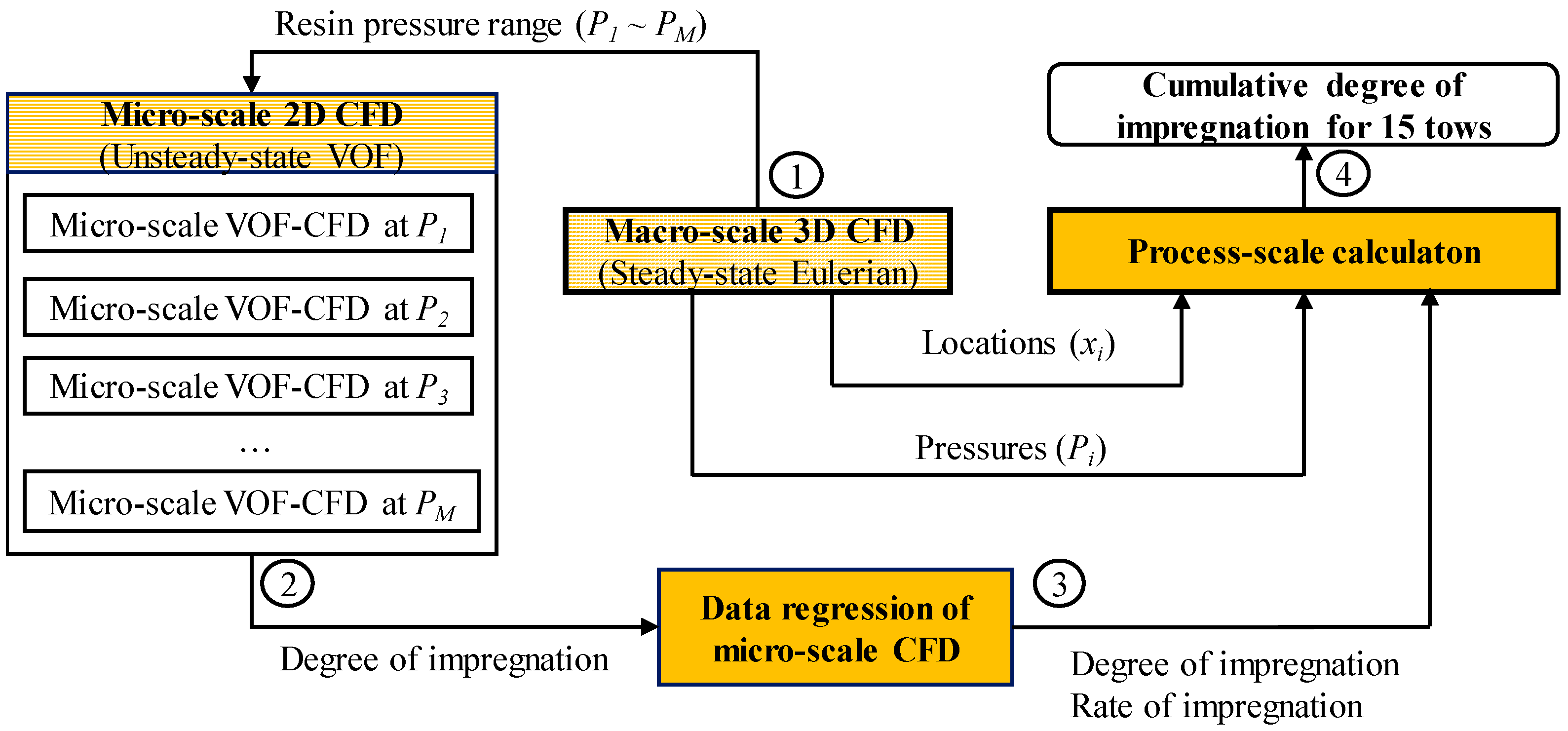
  29. Ngo, S.I.; Lim, Y.-I.; Hahn, M.-H.; Jung, J.; Bang, Y.-H. Multi-scale computational fluid dynamics of impregnation die for thermoplastic carbon fiber prepreg production. Comput. Chem. Eng. 2017, 103, 58–68. [Google Scholar] [CrossRef]
  30. Lakehal, D. Status and future developments of Large-Eddy Simulation of turbulent multi-fluid flows (LEIS and LESS). Int. J. Multiph. Flow 2018, 104, 322–337. [Google Scholar] [CrossRef]
  31. Xiao, H.; Cinnella, P. Quantification of model uncertainty in RANS simulations: A review. Prog. Aerosp. Sci. 2019, 108, 1–31. [Google Scholar] [CrossRef] [Green Version]
  32. Klein, M.; Ketterl, S.; Hasslberger, J. Large eddy simulation of multiphase flows using the volume of fluid method: Part 1—Governing equations and a priori analysis. Exp. Comput. Multiph. Flow 2019, 1, 130–144. [Google Scholar] [CrossRef] [Green Version]
  33. Ngo, S.I.; Lim, Y.-I.; Hahn, M.-H.; Jung, J. Prediction of degree of impregnation in thermoplastic unidirectional carbon fiber prepreg by multi-scale computational fluid dynamics. Chem. Eng. Sci. 2018, 185, 64–75. [Google Scholar] [CrossRef]
  34. da Rosa, C.A.; Braatz, R.D. Multiscale modeling and simulation of macromixing, micromixing, and crystal size distribution in radial mixers/crystallizers. Ind. Eng. Chem. Res. 2018, 57, 5433–5441. [Google Scholar] [CrossRef]
  35. Haghighat, A.; Luxbacher, K.; Lattimer, B.Y. Development of a methodology for interface boundary selection in the multiscale road tunnel fire simulations. Fire Technol. 2018, 54, 1029–1066. [Google Scholar] [CrossRef] [Green Version]
  36. Höhne, T.; Krepper, E.; Lucas, D.; Montoya, G. A multiscale approach simulating boiling in a heated pipe including flow pattern transition. Nucl. Technol. 2019, 205, 48–56. [Google Scholar] [CrossRef]
  37. Uribe, S.; Cordero, M.E.; Reyes, E.P.; Regalado-Méndez, A.; Zárate, L.G. Multiscale CFD modelling and analysis of TBR behavior for an HDS process: Deviations from ideal behaviors. Fuel 2019, 239, 1162–1172. [Google Scholar] [CrossRef]
  38. Ferreira, R.B.; Falcão, D.S.; Oliveira, V.B.; Pinto, A.M.F.R. Numerical simulations of two-phase flow in proton exchange membrane fuel cells using the volume of fluid method—A review. J. Power Sources 2015, 277, 329–342. [Google Scholar] [CrossRef]
  39. Karpinska, A.M.; Bridgeman, J. CFD-aided modelling of activated sludge systems—A critical review. Water Res. 2016, 88, 861–879. [Google Scholar] [CrossRef] [Green Version]
  40. Sharma, S.K.; Kalamkar, V.R. Computational fluid dynamics approach in thermo-hydraulic analysis of flow in ducts with rib roughened walls—A review. Renew. Sustain. Energy Rev. 2016, 55, 756–788. [Google Scholar] [CrossRef]
  41. Yin, C.; Yan, J. Oxy-fuel combustion of pulverized fuels: Combustion fundamentals and modeling. Appl. Energy 2016, 162, 742–762. [Google Scholar] [CrossRef]
  42. Uebel, K.; Rößger, P.; Prüfert, U.; Richter, A.; Meyer, B. CFD-based multi-objective optimization of a quench reactor design. Fuel Process. Technol. 2016, 149, 290–304. [Google Scholar] [CrossRef]
  43. Fotovat, F.; Bi, X.T.; Grace, J.R. Electrostatics in gas-solid fluidized beds: A review. Chem. Eng. Sci. 2017, 173, 303–334. [Google Scholar] [CrossRef]
  44. Pires, J.C.M.; Alvim-Ferraz, M.C.M.; Martins, F.G. Photobioreactor design for microalgae production through computational fluid dynamics: A review. Renew. Sustain. Energy Rev. 2017, 79, 248–254. [Google Scholar] [CrossRef]
  45. Malekjani, N.; Jafari, S.M. Simulation of food drying processes by Computational Fluid Dynamics (CFD); recent advances and approaches. Trends Food Sci. Technol. 2018, 78, 206–223. [Google Scholar] [CrossRef]
  46. Lu, B.; Niu, Y.; Chen, F.; Ahmad, N.; Wang, W.; Li, J. Energy-minimization multiscale based mesoscale modeling and applications in gas-fluidized catalytic reactors. Rev. Chem. Eng. 2019. [Google Scholar] [CrossRef]
  47. Wang, J. Continuum theory for dense gas-solid flow: A state-of-the-art review. Chem. Eng. Sci. 2020, 215, 115428. [Google Scholar] [CrossRef]
  48. Pham, H.H.; Lim, Y.-I.; Ngo, S.I.; Bang, Y.-H. Computational fluid dynamics and tar formation in a low-temperature carbonization furnace for the production of carbon fibers. J. Ind. Eng. Chem. 2019, 73, 286–296. [Google Scholar] [CrossRef]
  49. Farias, L.F.I.; de Souza, J.A.; Braatz, R.D.; da Rosa, C.A. Coupling of the population balance equation into a two-phase model for the simulation of combined cooling and antisolvent crystallization using OpenFOAM. Comput. Chem. Eng. 2019, 123, 246–256. [Google Scholar] [CrossRef]
  50. Ngo, S.I.; Lim, Y.-I.; Kim, S.-C. Wave characteristics of coagulation bath in dry-jet wet-spinning process for polyacrylonitrile fiber production using computational fluid dynamics. Processes 2019, 7, 314. [Google Scholar] [CrossRef] [Green Version]
  51. Wu, B.; Firouzi, M.; Mitchell, T.; Rufford, T.E.; Leonardi, C.; Towler, B. A critical review of flow maps for gas-liquid flows in vertical pipes and annuli. Chem. Eng. J. 2017, 326, 350–377. [Google Scholar] [CrossRef] [Green Version]
  52. Bhole, M.R.; Joshi, J.B.; Ramkrishna, D. CFD simulation of bubble columns incorporating population balance modeling. Chem. Eng. Sci. 2008, 63, 2267–2282. [Google Scholar] [CrossRef]
  53. Tran, B.V.; Nguyen, D.D.; Ngo, S.I.; Lim, Y.-I.; Kim, B.; Lee, D.H.; Go, K.-S.; Nho, N.-S. Hydrodynamics and simulation of air–water homogeneous bubble column under elevated pressure. AIChE J. 2019, 65, e16685. [Google Scholar] [CrossRef]
  54. Pham, D.A.; Lim, Y.-I.; Jee, H.; Ahn, E.; Jung, Y. Porous media Eulerian computational fluid dynamics (CFD) model of amine absorber with structured-packing for CO2 removal. Chem. Eng. Sci. 2015, 132, 259–270. [Google Scholar] [CrossRef]
  55. Ngo, S.I.; Lim, Y.-I.; Song, B.-H.; Lee, U.-D.; Lee, J.-W.; Song, J.-H. Effects of fluidization velocity on solid stack volume in a bubbling fluidized-bed with nozzle-type distributor. Powder Technol. 2015, 275, 188–198. [Google Scholar] [CrossRef]
  56. Ngo, S.I.; Lim, Y.-I.; Song, B.-H.; Lee, U.-D.; Yang, C.-W.; Choi, Y.-T.; Song, J.-H. Hydrodynamics of cold-rig biomass gasifier using semi-dual fluidized-bed. Powder Technol. 2013, 234, 97–106. [Google Scholar] [CrossRef]
  57. Sun, L.; Luo, K.; Fan, J. Numerical investigation on methanation kinetic and flow behavior in full-loop fluidized bed reactor. Fuel 2018, 231, 85–93. [Google Scholar] [CrossRef]
  58. Zhou, Q.; Wang, J. CFD study of mixing and segregation in CFB risers: Extension of EMMS drag model to binary gas–solid flow. Chem. Eng. Sci. 2015, 122, 637–651. [Google Scholar] [CrossRef]
  59. Gidaspow, D. Multiphase Flow and Fluidization: Continuum and Kinetic Theory Description; Academic Press: Cambridge, MA, USA, 1994. [Google Scholar]
  60. Lun, C.K.K.; Savage, S.B.; Jeffrey, D.J.; Chepurniy, N. Kinetic theories for granular flow: Inelastic particles in Couette flow and slightly inelastic particles in a general flowfield. J. Fluid Mech. 1984, 140, 223–256. [Google Scholar] [CrossRef]
  61. Syamlal, M.; Rogers, W.; O’Brien, T.J. MFIX Documentation: Volume1, Theory Guide; National Technical Information Service: Springfield, VA, USA, 1993. [Google Scholar]
  62. Schaeffer, D.G. Instability in the evolution equations describing incompressible granular flow. J. Differ. Equ. 1987, 66, 19–50. [Google Scholar] [CrossRef] [Green Version]
  63. Ogawa, S.; Umemura, A.; Oshima, N. On the equations of fully fluidized granular materials. Z. Angew. Math. Phys. ZAMP 1980, 31, 483–493. [Google Scholar] [CrossRef]
  64. Ge, W.; Wang, W.; Yang, N.; Li, J.; Kwauk, M.; Chen, F.; Chen, J.; Fang, X.; Guo, L.; He, X.; et al. Meso-scale oriented simulation towards virtual process engineering (VPE)-The EMMS Paradigm. Chem. Eng. Sci. 2011, 66, 4426–4458. [Google Scholar] [CrossRef]
  65. Hamidipour, M.; Chen, J.; Larachi, F. CFD study on hydrodynamics in three-phase fluidized beds—Application of turbulence models and experimental validation. Chem. Eng. Sci. 2012, 78, 167–180. [Google Scholar] [CrossRef]
  66. Hosseini, S.H.; Shojaee, S.; Ahmadi, G.; Zivdar, M. Computational fluid dynamics studies of dry and wet pressure drops in structured packings. J. Ind. Eng. Chem. 2012, 18, 1465–1473. [Google Scholar] [CrossRef]
  67. Nguyen, T.D.B.; Lim, Y.-I.; Kim, S.-J.; Eom, W.-H.; Yoo, K.-S. Experiment and Computational Fluid Dynamics (cfd) simulation of urea-based Selective Noncatalytic Reduction (SNCR) in a pilot-scale flow reactor. Energy Fuels 2008, 22, 3864–3876. [Google Scholar] [CrossRef]
  68. Ngo, S.I.; Lim, Y.-I.; Kim, W.; Seo, D.J.; Yoon, W.L. Computational fluid dynamics and experimental validation of a compact steam methane reformer for hydrogen production from natural gas. Appl. Energy 2019, 236, 340–353. [Google Scholar] [CrossRef]
  69. Rzehak, R.; Krauß, M.; Kováts, P.; Zähringer, K. Fluid dynamics in a bubble column: New experiments and simulations. Int. J. Multiph. Flow 2017, 89, 299–312. [Google Scholar] [CrossRef]
  70. Ramos, A.; Monteiro, E.; Rouboa, A. Numerical approaches and comprehensive models for gasification process: A review. Renew. Sustain. Energy Rev. 2019, 110, 188–206. [Google Scholar] [CrossRef]
  71. Kone, J.-P.; Zhang, X.; Yan, Y.; Hu, G.; Ahmadi, G. CFD modeling and simulation of PEM fuel cell using OpenFOAM. Energy Procedia 2018, 145, 64–69. [Google Scholar] [CrossRef]
  72. Ahmadi, S.; Sefidvash, F. Study of pressure drop in fixed bed reactor using a Computational Fluid Dynamics (CFD) code. Chem. Eng. 2018, 2, 14. [Google Scholar]
  73. Wang, J.-Q.; Ouyang, Y.; Li, W.-L.; Esmaeili, A.; Xiang, Y.; Chen, J.-F. CFD analysis of gas flow characteristics in a rotating packed bed with randomly arranged spherical packing. Chem. Eng. J. 2020, 385, 123812. [Google Scholar] [CrossRef]
  74. Kang, J.-L.; Ciou, Y.-C.; Lin, D.-Y.; Wong, D.S.-H.; Jang, S.-S. Investigation of hydrodynamic behavior in random packing using CFD simulation. Chem. Eng. Res. Des. 2019, 147, 43–54. [Google Scholar] [CrossRef]
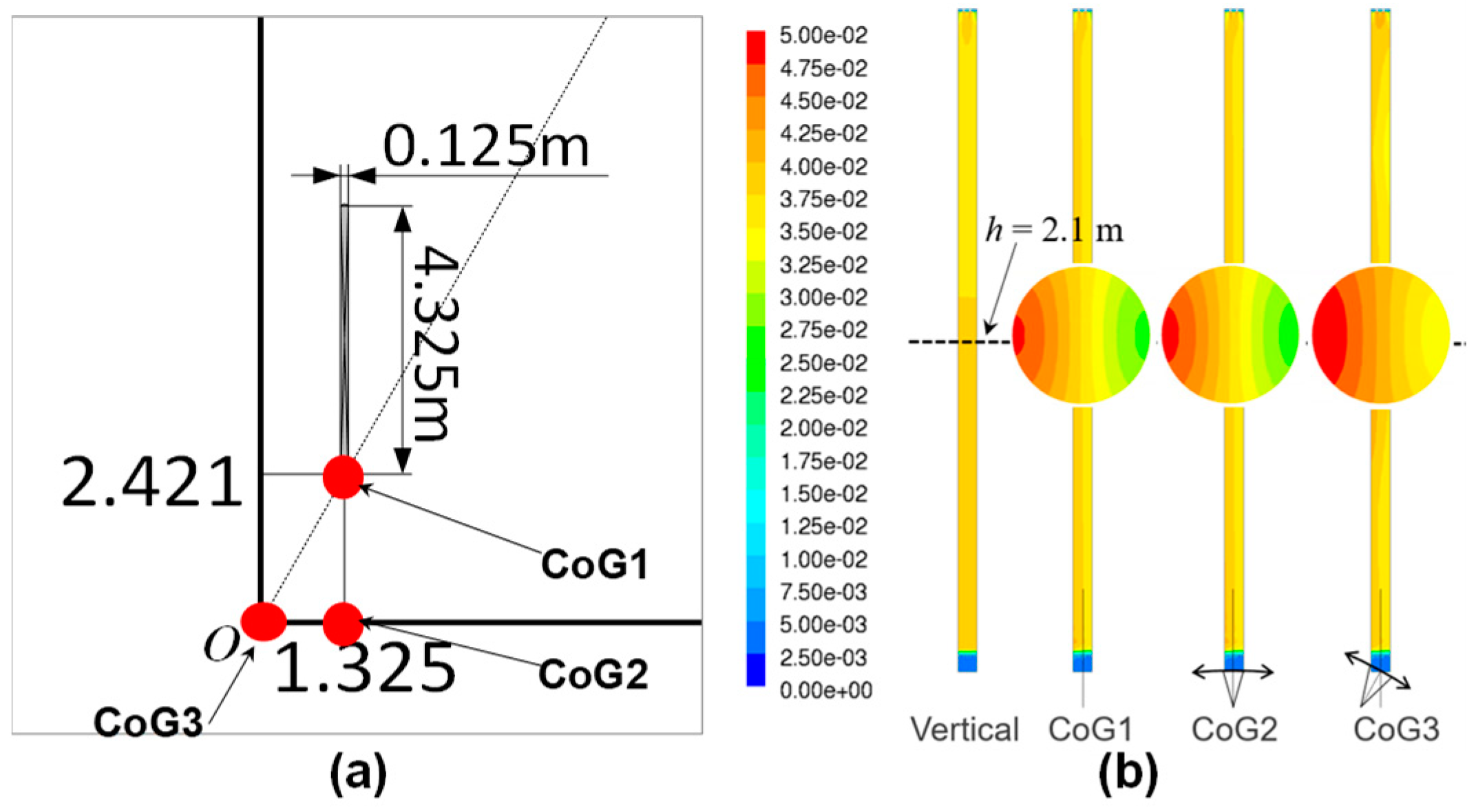
  75. Kim, J.; Pham, D.A.; Lim, Y.-I. Effect of gravity center position on amine absorber with structured packing under offshore operation: Computational fluid dynamics approach. Chem. Eng. Res. Des. 2017, 121, 99–112. [Google Scholar] [CrossRef]
  76. Soman, A.; Shastri, Y. Optimization of novel photobioreactor design using computational fluid dynamics. Appl. Energy 2015, 140, 246–255. [Google Scholar] [CrossRef]
  77. Le, T.T.; Ngo, S.I.; Lim, Y.-I.; Park, C.-K.; Lee, B.-D.; Kim, B.-G.; Lim, D.-H. Effect of simultaneous three-angular motion on the performance of an air–water–oil separator under offshore operation. Ocean Eng. 2019, 171, 469–484. [Google Scholar] [CrossRef]
  78. Fletcher, D.F.; McClure, D.D.; Kavanagh, J.M.; Barton, G.W. CFD simulation of industrial bubble columns: Numerical challenges and model validation successes. Appl. Math. Model. 2017, 44, 25–42. [Google Scholar] [CrossRef]
  79. Sharma, S.L.; Ishii, M.; Hibiki, T.; Schlegel, J.P.; Liu, Y.; Buchanan, J.R. Beyond bubbly two-phase flow investigation using a CFD three-field two-fluid model. Int. J. Multiph. Flow 2019, 113, 1–15. [Google Scholar] [CrossRef]
  80. Yan, P.; Jin, H.; He, G.; Guo, X.; Ma, L.; Yang, S.; Zhang, R. CFD simulation of hydrodynamics in a high-pressure bubble column using three optimized drag models of bubble swarm. Chem. Eng. Sci. 2019, 199, 137–155. [Google Scholar] [CrossRef]
  81. Thakare, H.R.; Monde, A.; Parekh, A.D. Experimental, computational and optimization studies of temperature separation and flow physics of vortex tube: A review. Renew. Sustain. Energy Rev. 2015, 52, 1043–1071. [Google Scholar] [CrossRef]
  82. Yang, X.; Yu, H.; Wang, R.; Fane, A.G. Optimization of microstructured hollow fiber design for membrane distillation applications using CFD modeling. J. Membr. Sci. 2012, 421–422, 258–270. [Google Scholar] [CrossRef] [Green Version]
  83. Minea, A.A.; Murshed, S.M.S. A review on development of ionic liquid based nanofluids and their heat transfer behavior. Renew. Sustain. Energy Rev. 2018, 91, 584–599. [Google Scholar] [CrossRef]
  84. Pham, H.H. Performance Evaluation of Low Temperature Furnace and Gas Distributors Using Computational Fluid Dynamics (CFD). Master Thesis, Hankyong National University, Anseong, Korea, 2018. [Google Scholar]
  85. Kim, J.; Pham, D.A.; Lim, Y.-I. Gas−liquid multiphase computational fluid dynamics (CFD) of amine absorption column with structured-packing for CO2 capture. Comput. Chem. Eng. 2016, 88, 39–49. [Google Scholar] [CrossRef]
  86. Zhang, G.; Jiao, K. Multi-phase models for water and thermal management of proton exchange membrane fuel cell: A review. J. Power Sources 2018, 391, 120–133. [Google Scholar] [CrossRef]
  87. Li, W.-L.; Ouyang, Y.; Gao, X.-Y.; Wang, C.-Y.; Shao, L.; Xiang, Y. CFD analysis of gas–liquid flow characteristics in a microporous tube-in-tube microchannel reactor. Comput. Fluids 2018, 170, 13–23. [Google Scholar] [CrossRef]
  88. Bhusare, V.H.; Dhiman, M.K.; Kalaga, D.V.; Roy, S.; Joshi, J.B. CFD simulations of a bubble column with and without internals by using OpenFOAM. Chem. Eng. J. 2017, 317, 157–174. [Google Scholar] [CrossRef]
  89. Behkish, A.; Lemoine, R.; Sehabiague, L.; Oukaci, R.; Morsi, B.I. Gas holdup and bubble size behavior in a large-scale slurry bubble column reactor operating with an organic liquid under elevated pressures and temperatures. Chem. Eng. J. 2007, 128, 69–84. [Google Scholar] [CrossRef]
  90. Zhang, H.; Yang, G.; Sayyar, A.; Wang, T. An improved bubble breakup model in turbulent flow. Chem. Eng. J. 2019. [Google Scholar] [CrossRef]
  91. Abdelmotalib, H.M.; Youssef, M.A.M.; Hassan, A.A.; Youn, S.B.; Im, I.-T. Heat transfer process in gas–solid fluidized bed combustors: A review. Int. J. Heat Mass Transf. 2015, 89, 567–575. [Google Scholar] [CrossRef]
  92. Wu, Y.; Shi, X.; Liu, Y.; Wang, C.; Gao, J.; Lan, X. 3D CPFD simulations of gas-solids flow in a CFB downer with cluster-based drag model. Powder Technol. 2019. [Google Scholar] [CrossRef]
  93. Banerjee, S.; Agarwal, R.K. Computational fluid dynamics modeling and simulations of fluidized beds for chemical looping combustion. In Handbook of Chemical Looping Technology; Breault, R.W., Ed.; Wiley-VCH: Weinheim, Germany, 2020; pp. 303–332. [Google Scholar] [CrossRef]
  94. Andrews, M.J.; O’Rourke, P.J. The multiphase particle-in-cell (MP-PIC) method for dense particulate flows. Int. J. Multiph. Flow 1996, 22, 379–402. [Google Scholar] [CrossRef]
  95. Snider, D.M.; Clark, S.M.; O’Rourke, P.J. Eulerian–Lagrangian method for three-dimensional thermal reacting flow with application to coal gasifiers. Chem. Eng. Sci. 2011, 66, 1285–1295. [Google Scholar] [CrossRef]
  96. Kim, S.H.; Lee, J.H.; Braatz, R.D. Multi-phase particle-in-cell coupled with population balance equation (MP-PIC-PBE) method for multiscale computational fluid dynamics simulation. Comput. Chem. Eng. 2020, 134, 106686. [Google Scholar] [CrossRef]
  97. Li, Y.; Yang, G.Q.; Zhang, J.P.; Fan, L.S. Numerical studies of bubble formation dynamics in gas–liquid–solid fluidization at high pressures. Powder Technol. 2001, 116, 246–260. [Google Scholar] [CrossRef]
  98. Chen, L.; Feng, Y.-L.; Song, C.-X.; Chen, L.; He, Y.-L.; Tao, W.-Q. Multi-scale modeling of proton exchange membrane fuel cell by coupling finite volume method and lattice Boltzmann method. Int. J. Heat Mass Transf. 2013, 63, 268–283. [Google Scholar] [CrossRef]
  99. Pozzetti, G.; Peters, B. A multiscale DEM-VOF method for the simulation of three-phase flows. Int. J. Multiph. Flow 2018, 99, 186–204. [Google Scholar] [CrossRef]
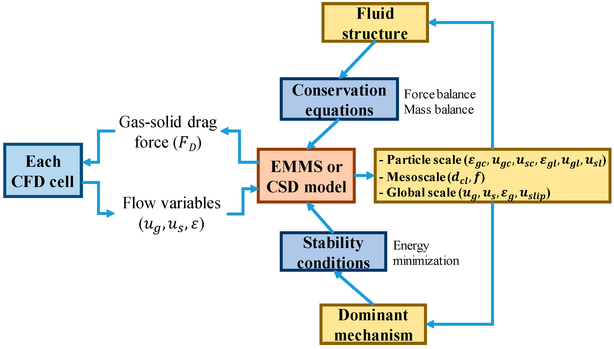
  100. Qi, H.; Li, F.; Xi, B.; You, C. Modeling of drag with the Eulerian approach and EMMS theory for heterogeneous dense gas-solid two-phase flow. Chem. Eng. Sci. 2007, 62, 1670–1681. [Google Scholar] [CrossRef]
  101. Raynal, L.; Royon-Lebeaud, A. A multi-scale approach for CFD calculations of gas–liquid flow within large size column equipped with structured packing. Chem. Eng. Sci. 2007, 62, 7196–7204. [Google Scholar] [CrossRef]
  102. Qi, W.; Guo, K.; Liu, C.; Liu, H.; Liu, B. Liquid distribution and local hydrodynamics of winpak: A multiscale method. Ind. Eng. Chem. Res. 2017, 56, 15184–15194. [Google Scholar] [CrossRef]
  103. Gao, X.; Li, T.; Sarkar, A.; Lu, L.; Rogers, W.A. Development and validation of an enhanced filtered drag model for simulating gas-solid fluidization of Geldart A particles in all flow regimes. Chem. Eng. Sci. 2018, 184, 33–51. [Google Scholar] [CrossRef]
  104. Lu, B.; Wang, W.; Li, J. Searching for a mesh-independent sub-grid model for CFD simulation of gas–solid riser flows. Chem. Eng. Sci. 2009, 64, 3437–3447. [Google Scholar] [CrossRef]
  105. Wang, W.; Li, J. Simulation of gas–solid two-phase flow by a multi-scale CFD approach—Of the EMMS model to the sub-grid level. Chem. Eng. Sci. 2007, 62, 208–231. [Google Scholar] [CrossRef]
  106. Bernaschi, M.; Melchionna, S.; Succi, S.; Fyta, M.; Kaxiras, E.; Sircar, J.K. MUPHY: A parallel MUlti PHYsics/scale code for high performance bio-fluidic simulations. Comput. Phys. Commun. 2009, 180, 1495–1502. [Google Scholar] [CrossRef]
  107. Tang, Y.-H.; Kudo, S.; Bian, X.; Li, Z.; Karniadakis, G.E. Multiscale universal interface: A concurrent framework for coupling heterogeneous solvers. J. Comput. Phys. 2015, 297, 13–31. [Google Scholar] [CrossRef] [Green Version]
  108. Neumann, P.; Flohr, H.; Arora, R.; Jarmatz, P.; Tchipev, N.; Bungartz, H.-J. MaMiCo: Software design for parallel molecular-continuum flow simulations. Comput. Phys. Commun. 2016, 200, 324–335. [Google Scholar] [CrossRef]
  109. Neumann, P.; Bian, X. MaMiCo: Transient multi-instance molecular-continuum flow simulation on supercomputers. Comput. Phys. Commun. 2017, 220, 390–402. [Google Scholar] [CrossRef]
  110. Li, L.; Li, B.; Liu, Z. Modeling of spout-fluidized beds and investigation of drag closures using OpenFOAM. Powder Technol. 2017, 305, 364–376. [Google Scholar] [CrossRef]
  111. Lu, Y.; Liu, C.; Wang, K.I.K.; Huang, H.; Xu, X. Digital twin-driven smart manufacturing: Connotation, reference model, applications and research issues. Robot. Comput. Integr. Manuf. 2020, 61, 101837. [Google Scholar] [CrossRef]
  112. Negri, E.; Fumagalli, L.; Macchi, M. A review of the roles of digital twin in CPS-based production systems. Procedia Manuf. 2017, 11, 939–948. [Google Scholar] [CrossRef]
  113. Katz, A.; Sankaran, V. Mesh quality effects on the accuracy of CFD solutions on unstructured meshes. J. Comput. Phys. 2011, 230, 7670–7686. [Google Scholar] [CrossRef]
  114. Roache, P.J. Perspective: A method for uniform reporting of grid refinement studies. J. Fluids Eng. 1994, 116, 405–413. [Google Scholar] [CrossRef]
  115. Roache, P.J. Verification of codes and calculations. AIAA J. 1998, 36, 696–702. [Google Scholar] [CrossRef]
  116. Owens, S.A.; Perkins, M.R.; Eldridge, R.B.; Schulz, K.W.; Ketcham, R.A. Computational fluid dynamics simulation of structured packing. Ind. Eng. Chem. Res. 2013, 52, 2032–2045. [Google Scholar] [CrossRef]
  117. Cloete, S.; Johansen, S.T.; Amini, S. Grid independence behaviour of fluidized bed reactor simulations using the two fluid model: Detailed parametric study. Powder Technol. 2016, 289, 65–70. [Google Scholar] [CrossRef] [Green Version]
  118. Liu, Q.; Gómez, F.; Pérez, J.M.; Theofilis, V. Instability and sensitivity analysis of flows using OpenFOAM®. Chin. J. Aeronaut. 2016, 29, 316–325. [Google Scholar] [CrossRef] [Green Version]
  119. Wang, J.-X.; Xiao, H. Data-driven CFD modeling of turbulent flows through complex structures. Int. J. Heat Fluid Flow 2016, 62, 138–149. [Google Scholar] [CrossRef] [Green Version]
Figure 1. Impregnation die for carbon fiber (CF) tape production from a multiscale point of view (modified from Ngo et al. (2018) [33]). (a) CF tape; (b) impregnation die; (c) mesh structure around one tow; and (d) CF tow representative element volume (REV) on a microscale.
Chemengineering 04 00023 g001
Figure 2. Schoepentoeter gas distributor used in an amine absorber. (a) Gas distributor with Schoepentoeter; (b) gas velocity vector around Schoepentoeter; and (c) radial velocity contour above chimney tray (modified from Pham et al. (2018) [24]).
Chemengineering 04 00023 g002
Figure 3. Amine absorber with structured-packing under off-shore operation. (a) Layout of amine absorber with three centers of gravity (CoG); and (b) liquid holdup contour under pitching motion at h = 2.1 m for three CoGs (modified from Kim et al. (2017) [75]).
Chemengineering 04 00023 g003
Figure 4. Gas holdup contours in air-water homogeneous bubble column at 1–35 bar (modified from Tran et al. (2019) [53]).
Chemengineering 04 00023 g004
Figure 5. Concurrent coupling strategy of multiscale Eulerian CFD with energy minimization multi-scale (EMMS) or cluster structure-dependent (CSD) in fluidized beds (modified from Li et al. (2018) [87,100]).
Chemengineering 04 00023 g005
Figure 6. Sequential coupling strategy of multiscale CFD simulation to predict the permeability of resin through porous tows for the production of thermoplastic carbon fibers (modified from Ngo et al. (2017) [29]).
Chemengineering 04 00023 g006
Figure 7. Sequential coupling strategy of multiscale CFD simulation to predict the degree of resin impregnation for the production of thermoplastic carbon fiber (modified from Ngo et al. (2018) [33]).
Chemengineering 04 00023 g007
Figure 8. Sequential coupling strategy of a multiscale Eulerian CFD with EMMS in fluidized beds (modified from Lu et al. (2009) [104,105]).
Chemengineering 04 00023 g008
Table 1. Single-phase Eulerian computational fluid dynamics (CFD) model [24,48].
Continuity equation: ρ · u = 0 (T1-1)
Momentum equation: ρ t u = ρ · ( u u ) P + · τ = + ρ g
where τ = = ( μ + μ t ) [ ( u + u T 2 3 ( · u ) I = ) 2 3 ρ k I =
(T1-2)
Energy equation: ρ c p T t = · u ( ρ c p T + P ) + · ( λ T + τ = · u ) ± S h (T1-3)
Table 2. Volume of fluid (VOF)-CFD model for gas-liquid phase [33,50].
Continuity equation: · u = 0 (T2-1)
Volume fraction equation: α L t = · ( α L u ) · u c α L ( 1 α L )
    where the sharpening velocity ( u c ) is u c = C u α L α L and α L + α G = 1
(T2-2)
Momentum equation:
  ρ t u = ρ · ( u u ) P + ( μ + μ t ) · [ ( u + u T ) 2 3 ( · u ) I = ] 2 3 ρ k I = + ρ g + F s u r f
(T2-3)
    where the surface tension force is F s u r f = · τ = s u r f (T2-4)
    with the surface stress tensor of τ = s u r f = σ ( | α L | I = α L · ( α L ) T | α L | ) (T2-5)
Energy equation: ρ E t = ρ · u E + · ( λ T + τ = · u ) ± S h (T2-6)
Single properties (density): ρ = α G ρ G + α L ρ L (T2-7)
        (viscosity): μ = α G μ G + α L μ L
        (conductivity): λ = α G λ G + α L λ L
        (energy): E = ( α G ρ G E G + α L ρ L E L ) / ρ
(T2-8)
(T2-9)
(T2-10)
Table 3. Eulerian multiphase (EM)-CFD model for gas-liquid phase [53,54].
Continuity equation: ρ G t ( α G ) = ρ G · ( α G u G )
α L = 1 α G
(T3-1)
Momentum equation: ρ G t ( α G u G ) = ρ G · ( α G u G u G ) α G P + · τ = G + ρ G α G g F G L
ρ L t ( α L u L ) = ρ L · ( α L u L u L ) α L P + · τ = L + ρ L α L g + F G L
where τ = G = α G μ G ( u G + u G T 2 3 ( · u G ) I = ) 2 3 ρ G k I = ,
τ = L = α L μ L ( u L + u L T 2 3 ( · u L ) I = ) 2 3 ρ L k I = ,
(T3-2)
F G L = F D + F L + F W + F T ,(T3-3)
F D = K G L ( u G u L ) ,   K G L = 3 4 C D d b ρ L α G α L | u G u L | ,(T3-4)
F L = C L ρ L α G ( u L u G ) × ( × u L ) ,(T3-5)
F W = C W ρ L α G | ( u L u G ) w a l l | 2 n W ,(T3-6)
and F T = C T K G L μ t , L σ G L ρ L ( α G α G α L α L ) (T3-7)
Energy equation: ρ G α G E G t = ρ G · u G α G E G + · ( α G λ G T G + τ = G · u G ) Q G L ± S h , G (T3-8)
        ρ L α L E L t = ρ L · u L α L E L + · ( α L λ L T L + τ = L · u L ) + Q G L ± S h , L (T3-9)
Table 4. Kinetic theory of granular flow (KTGF)-CFD model for gas-solid phases [55,58].
Continuity equation (gas phase): ( 1 α ) t + · ( ( 1 α ) u ) = 0
         (solid phase): α t + · ( α v ) = 0
(T4-1)
Momentum equation (gas phase): ρ G ( ( 1 α ) u ) t = ρ G · ( ( 1 α ) u u ) ( 1 α ) p + · ( τ G = ) + ρ G ( 1 α ) g F D , G S
         (solid phase): ρ S ( α v ) t = ρ S · ( α v v ) α p p S + · ( τ S = ) + ρ S α g + F D , G S
(T4-2)
  where the solid-gas drag [59] is F D , G S = K G S ( u v ) , K G S = 3 4 C D ρ G ( 1 α ) α | u v | d ( 1 α ) 2.65
    when 1 α > 0.8 (dilute), with C D = 24 ( 1 α ) R e s [ 1 + 0.15 ( ( 1 α ) R e s ) 0.687 ] ,
     K G S = 150 α 2 μ G ( 1 α ) d 2 + 1.75 α ρ G | u v | d when 1 α 0.8 (dense),
(T4-3)
 the gas-phase stress tensor is τ G = = ( 1 α ) μ G [ u + u T 2 3 ( · u ) I = ] 2 3 ρ G k I = ,(T4-4)
 the solid-phase stress tensor is τ S = = [ p S + α λ S · v ] I = α μ S [ v + v T 2 3 ( · v ) I = ] 2 3 ρ G k I = ,(T4-5)
 the solid-phase pressure is p S = α ρ S [ 1 + 2 ( 1 + e ) α g 0 ] Θ ,(T4-6)
 the solid-phase bulk viscosity [60] is λ S = 4 3 α ρ S d g 0 ( 1 + e ) ( Θ π ) 1 2 ,(T4-7)
 the solid shear viscosity is μ S = μ S , c o l + μ S , k i n + μ S , f r i ,(T4-8)
 the collision viscosity of solids [61] is μ S , c o l = 4 5 α ρ S d g 0 ( 1 + e ) ( Θ π ) 1 2 ,(T4-9)
 the kinetic viscosity of solids [59] is μ S , k i n = 10 ρ S d Θ π 96 α ( 1 + e ) g 0 [ 1 + 4 5 g 0 α ( 1 + e ) ] 2 α ,(T4-10)
 the frictional viscosity of solids [62] is μ S , f r i = p s s i n ϕ 2 I 2 D ; with ϕ = 30 0 ,(T4-11)
 and the radial distribution function [63] is g 0 = [ 1 ( α α m ) 1 3 ] 1 with the maximum packing ( α m )(T4-12)
Granular temperature ( Θ ) equation neglecting the convection and diffusion terms: 0 = ( p S I = + τ S = ) : v γ S + ϕ G S (T4-13)
  where the energy generation by the solid stress tensor ( τ S = ) with a double inner product is ( p S I = + τ S = ) : v ,(T4-14)
  the energy collisional dissipation rate of the solid phase [60] is γ S = 12 ( 1 e 2 ) g 0 d π ρ S α 2 Θ 3 2 ,(T4-15)
  and the fluctuation kinetic energy transfer from the solid to gas phase [59] is ϕ G S = 3 K G S Θ (T4-16)
Energy equation: ρ G ( 1 α ) E G t = ρ G · u ( 1 α ) E G + · ( ( 1 α ) λ G T G + τ = G · u ) Q G S ± S h , G (T4-17)
       ρ S α E S t = ρ S · v α E S + · ( α λ S T S + τ = S · v ) + Q G S ± S h , S (T4-18)
Table 5. EM-KTGF-CFD model for gas-liquid-solid phases [65].
Continuity equation (gas phase): ρ G α G t = ρ G · ( α G u G )
          (liquid phase): ρ L α L t = ρ L · ( α L u L )
          (solid phase): ρ S α S t = ρ S · ( α S u S )
(T5-1)
Momentum equation (gas phase): ρ G ( α G u G ) t = ρ G · ( α G u G u G ) α G p + · τ G = + ρ G α G g F D , G L F D , G S
          (liquid phase): ρ L ( α L u L ) t = ρ L · ( α L u L u L ) α L P + · τ = L + ρ L α L g + F D , G L F D , L S
          (solid phase): ρ S ( α S u S ) t = ρ S · ( α S u S u S ) α S p p S + · τ S = + ρ S α S g + F D , L S + F D , G S
(T5-2)
Interface interactions (G-L): F D , G L = K G L ( u G u L ) ,   K G L = 3 4 C D , G L d b ρ L α G α L | u G u L |
    (S-L): F D , S L = K S L ( u S u L ) ,   K S L = 3 4 C D , S L ρ L α S α L | u S u L | d s α L 2.65   f o r   α L > 0.8 ,  
                   a n d   K S L = 150 α S ( 1 α L ) μ L α L d s 2 + 1.75 α S ρ L | u S u L | d s   f o r   α L 0.8
    (G-S): F D , G S = K G S ( u G u S ) , K G S = 3 4 C D , G S d s ρ g α G α S | u G u L |
(T5-3)
Energy equation (gas phase): ρ G α G E G t = ρ G · u G α G E G + · ( α G λ G T G + τ = G · u G ) Q G L Q G S ± S h , G
        (liquid phase): ρ L α L E L t = ρ L · u L α L E L + · ( α L λ L T L + τ = L · u L ) + Q G L Q L S ± S h , L
        (solid phase): ρ S α S E S t = ρ S · u S α S E s + · ( α S λ s T s + τ = s · u S ) + Q L S + Q G S ± S h , S
(T5-4)
Table 6. Recent progress of multiscale CFD simulation of chemical and biological processes.
AdvantageDisadvantageAuthorModelsApplication Field
Concurrent couplingHigh accuracyHigh computational costChen, 2013 [98]LBM-CFDPEM fuel cell
Crose, 2017 [13]KMC-CFDPECVD wafer
Pozzetti, 2018 [99]DEM-VOFThree-phase flows with particles
Da Rosa, 2018 [34]PBE-CFDTubular crystallizer
Qi, 2007 [100]EMMS-CFDFluidized beds
Li, 2018 [87]CSD-CFDFluidized beds
Sequential couplingLow accuracyLow computational costRaynal, 2007 [101]VOF-EM-CFDAbsorber with structured packing
Ngo, 2017 [29]Eulerian CFDImpregnation die for carbon fiber
Ngo, 2018 [33]VOF-CFDImpregnation die for carbon fiber
Qi, 2017 [102]VOF-UNMAbsorber with structure packing
Wang, 2007 [105]EMMS-CFDFluidized beds
Lu, 2009 [104]EMMS-CFDFluidized beds

