Drying Technology Assisted by Nonthermal Pulsed Filamentary Microplasma Treatment: Theory and Practice

Abstract

Nonthermal pulsed filamentary microplasma treatment for drying is a nonthermal technology with promising perspectives to dehydrate plant agricultural materials. The modified set of Luikov’s equations for heat, mass and pressure transfer, has been used to analyze nonthermal pulsed filamentary microplasma treatment effects. The finite element method in combination with the step-by-step finite-difference method for a coupled system of differential equations in partial derivatives was used for numerical simulation of heat, humidity and pressure potentials transfer. The drying time of samples treated by nonthermal pulsed filamentary microplasma treatment assisted by thermionic emission was reduced up to 20.6% (5 kV/cm; 1200 discharges) in comparison to intact tissue. The effect of the obtained approach is very useful for studying process mechanisms and for explaining nonthermal pulsed filamentary microplasma treatment effects. Refined transfer kinetic coefficients from a set of equations based on experimental drying curve can be used for the quantitative determination of thermodynamic coefficients. The agreement of the simulation data with the analytical equation and experimental results is satisfactory (discrepancy less than 3%). Obtained results showed that the proposed model with the refined transfer kinetic coefficients adequately describe the experimental data.

1. Introduction

From the view of thermodynamic processes, preliminary electrical treatment promotes mass transfer process intensification in applications such as nonthermal pulsed filamentary microplasma (NTPFM) treatment assisted by thermionic emission (TE). Primary explanation of this effect is possible in terms of the volume porosity changes in material structure. There are two main phenomena that can be produced when an external electric field is applied to a biological tissue: electroporation and electrocompression [1]. NTPFM treatment effect is an alternative to pulsed electric field treatment effect, known as electroporation, and has been attributed to creation of perforating pathways in the lipid bilayer along direction of electric field. The formation of new pathways in treatment zones promotes changes of the general diffusion of a mass transfer process [2]. This fact was observed experimentally. During the experiment, it was seen that the volume of released intracellular liquid (in the case of a biological object consideration) has a significant amount and depends on the value of intracellular turgor pressure and treatment duration. Other explanations of a mass transfer process intensification after preliminary treatment by nonthermal pulsed filamentary microplasma can be characterized as a process of the plant cell membranes electroporation (locally at the treatment zone) at the expense of the formed transmembrane potential [3,4,5,6,7,8,9,10]. For such an analysis, the index of disintegration (quantity of the destroyed cell membranes) [11] can be used based on change of material conductivity before and after treatment.

Recently, several nonthermal pretreatment methods, such as pulse electric field (PEF) and cold plasma treatment have been proposed for potato dewatering enhancement in the drying processes [12,13,14,15]. The main explanation of PEF treatment effect was observed by describing effective moisture diffusion coefficient, which then was fitted to the Arrhenius law [12]. Liu C et al. reported interesting data of convective and microwave potato drying in combination with pulsed electric field treatment. It was observed that electroporation affects the heat and mass transfer processes during the different drying periods. Few authors reported effect of cold plasma for a drying process [14,15]. Zhang et al. treated species of chili pepper with a plasma flow of 20 kHz with a power consumption of 750 W. It was found that the drying time of pretreated samples was reduced by 12.6% (for target moisture of 20%) compared to the nontreated chili samples. Li S et al. treated corn kernels with a cold plasma pretreatment power of 500 W during 50 s. The results showed that cold plasma pretreatment can significantly reduce the drying time and improve the drying efficiency.

However, to the best of our knowledge, all reported research, both for PEF and cold plasma are based on mass and temperature transfer effects after treatment. No previous reports have been found regarding the pressure after NTPFM treatment.

In recent years, a consensus has been reached that a drying process is the one with the simultaneous transport of heat, free water, bound water, vapor water and air and that the complete description of drying process requires using three coupled nonlinear differential equations to account for the effect of temperature, humidity and pressure fields. Khan et al. (2017) reported an experimental investigation of bound and free water transport processes during potato drying [16]. In some cases with drying in an electric field, the electrodiffusion coefficient can be included [17].

Lykov suggested a three-way coupled heat, mass and pressure transfer model, formulated on irreversible thermodynamics processes. Analytical solutions of Luikov heat and mass transfer differential equation system are only available for simple geometrical configurations and boundary conditions [18]. The numerical solution of this task is possible by developing a pluripotential system of coupled differential equations and by the modification of it to a symmetric system.

Such an approach is very useful to study the mechanism of drying process, an explanation of the evolving effects. Using specified kinetic coefficients from experimental data, the biomaterials drying process with NTPFM treatment can be explained.

2. Materials and Methods

2.1. Sample Preparation

Commercial potatoes (Borovichok) were purchased in a local supermarket (Krasnodar, Russia). The wet basis (wb) initial water content in potato (wb = 0.84 ± 0.01 g/g), was determined by the oven method [19]. About 50 g of the fresh tissue were ground and dried in a hot air oven at 103 ± 2 °C for about 3 h until the differences between two weights was slight (± 0.05 g). The potato disks (40 mm in diameter and 4 mm in thickness) were manually prepared before experiments using the special cylindrical knife.

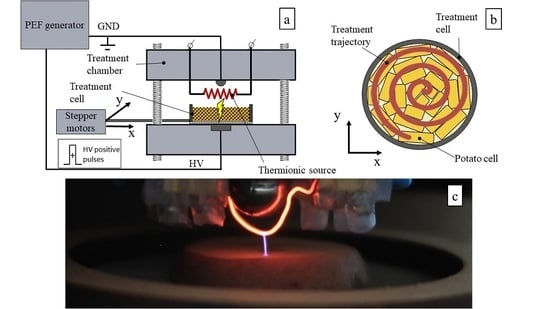
2.2. Nonthermal Pulsed Filamentary Microplasma Treatment Assisted by TE

NTPFM treatment was applied using pilot PEF system (PulseTech, Riceshell Inc., Krasnodar, Russian Federation) as described in [20] assisted by thermionic emission (TE). Pilot PEF-system based on a 1 kW Matsusada pulse generator (MASTSUSADA, Precision Inc., Shiga, Japan) that produces monopolar retangular electric pulses of 30 µs with a 100 Hz frequency at a maximum peak voltage of 20 kV. Total NTPFM treatment time was 2 min for each sample with electric field of E = 5 kV/cm. Applied electric pulses characteristics such as pulse frequency, pulse width, pulse pause time and amplitude were monitored by a digital oscilloscope (Tektronix TBS 2072, Beaverton, OR, USA) with P6015A oscilloscope probe (X1000, 400 MHz).

Thermionic emission was supported by wire coil type heat conductor made from nickel (wire diameter: 1 mm). Five volts and 3 amperes were applied to heated wire-coil up to 900 °C. Total specific input energy was 1.4 kJ/kg for 1200 applied discharges (Figure 1c). Total treatment time was set to 30 s to minimize influence of the heated coil on drying process. Difference in temperature between untreated and NTPFM-treated material was less than 3 °C (on the surface from the thermionic source side).

The principle of the experimental set-up is described in Figure 1a. In order to generate pulsed filamentary plasma in the air gap, a point-to-point electrode configuration was used, constituted by two stainless steel spheres (10 mm in diameter each) connected to a permanent magnet (to focus current flow) as a HV and GRD electrodes in a dielectric holder. The 2-cm electrode gap was set. The treatment cell was cylindrically formed (50 mm in diameter) and made from dielectric material (wood). The bottom of the cell was made of dielectric wire mesh for passage of electrical discharges. The treatment cell was set on a positioning platform with two Mercury stepper motors. The trajectory of treatment cell movements was set in accordance with Figure 1b. Trajectory was set for the maximum coverage area of the sample (Figure 1b).

2.3. Drying

Drying was done in a gravity convection drying oven (ED 53, Binder, Tuttlingen, Germany) at temperature of 105 °C. Control and PEF-treated potato samples were placed in to the glass chamber and kept inside the dryer. Then, the moisture loss of the potato samples was measured at 5 min intervals during the drying experiment using digital weighing balance. Drying continued until the final moisture content of the samples reached approximately 5% (wb). The moisture ratio (MR) of potato samples during drying was calculated as:

$$MR=\frac{m_t-m_e}{m_0-m_e}$$

(1)

where m_t, m₀, and m_e are moisture content at any time t (kg water/kg dry matter), initial moisture content (kg water/kg dry matter), and equilibrium moisture content (kg water/kg dry matter), respectively. Thermodynamic methods for moisture analysis transfer are based on the concept of potential. Transfer potential is a function of the state of the system and is equal at all points of the system at equilibrium. The potential gradient determines the direction and transfer rate of the corresponding substance [18]. By analogy with heat transfer, in which thermodynamical methods of analysis are successfully applied, the concept of mass content is similar to heat content. Briefly, moisture potential determination was based on finding the mass content of the sample in contact with a reference sample, for which the maximum specific sorption mass content is equal to 100 units. Obtained moisture content of potato samples was transformed in to moisture potential using Luikov expression [18]:

$$m=c_{m}M$$

(2)

where M is the moisture potential (°M). Parameter c_m is a material property termed “the specific moisture capacity” (kg of moisture/kg of dry matter °M) by Luikov [18]. The value of c_m, is usually determined experimentally based on using a reference scale built on the hygroscopic properties of filter paper upon Equation (2) or can be taken from literature.

2.4. Statistical Analysis

The experiments were replicated at least three times. All statistical analyses, evaluation of the mean values and standard deviations were calculated using IBM SPSS Statistics Subscription software. The error bars in all figures correspond to the confidence level of 95%. For derivation of drying data, the curve fitting software MagicPlot v.2.9 was used.

3. Theory

3.1. Problem Definition

In experiments with nonthermal pulsed filamentary microplasma, the effect on the drying process as a pretreatment method influence of pressure cannot be neglected. Luikov’s heat and mass transfer model in capillary porous media has been successfully employed to simulate temperature and moisture movement in food grains. The coupled partial differential equation system for temperature, moisture and pressure is formed by equations [21]:

$$\frac{\partial \mathrm{T}}{\partial \mathrm{t}}=\frac{\in \mathsf{\lambda }{c}_m\mathrm{D}}{{\mathrm{c}}_{\mathrm{q}}}{\nabla }^2\mathrm{M}+\left(\frac{{\mathrm{k}}_{\mathrm{q}}}{{\mathsf{\rho }}_0{\mathrm{c}}_{\mathrm{q}}}+\frac{\in \mathsf{\lambda }\mathsf{\delta }\mathrm{D}}{{\mathrm{c}}_{\mathrm{q}}}\right){\nabla }^2\mathrm{T}+\frac{\in {\mathsf{\lambda }\mathrm{k}}_{\mathrm{p}}}{{\mathsf{\rho }}_0{\mathrm{c}}_{\mathrm{q}}}{\nabla }^2\mathrm{P}$$

(3)

$$\frac{\partial \mathrm{M}}{\partial \mathrm{t}}=\mathrm{D}{\nabla }^2\mathrm{M}+\frac{\mathsf{\delta }\mathrm{D}}{c_m}{\nabla }^2\mathrm{T}+\frac{{\mathrm{k}}_{\mathrm{P}}}{{\mathsf{\rho }}_0{c}_m}{\nabla }^2\mathrm{P}$$

(4)

$$\frac{\partial \mathrm{P}}{\partial \mathrm{t}}=-\frac{\mathrm{D}\in c_m}{{\mathrm{c}}_{\mathrm{p}}}{\nabla }^2\mathrm{M}+\frac{\mathrm{D}\in \mathsf{\delta }}{{\mathrm{c}}_{\mathrm{p}}}{\nabla }^2\mathrm{T}+\frac{{\mathrm{k}}_{\mathrm{p}}}{{\mathsf{\rho }}_0{\mathrm{c}}_{\mathrm{p}}}\left(1-\in \right){\nabla }^2\mathrm{P}$$

(5)

The system is asymmetric, which makes difficult to solve numerically. However, multiplying Equation (3) by ${\mathrm{C}}_{\mathrm{q}}={\mathsf{\rho }}_0{\mathrm{c}}_{\mathrm{q}}\mathsf{\delta }/c_m$ Equation (4) by ${\mathrm{C}}_{\mathrm{m}}=\in {\mathsf{\lambda }\mathsf{\rho }}_0{c}_m$ and Equation (5) by ${\mathrm{C}}_{\mathrm{p}}=-{\mathsf{\lambda }\mathsf{\rho }}_0{\mathrm{c}}_{\mathrm{p}}{\mathrm{k}}_{\mathrm{p}}/{\mathrm{k}}_{\mathrm{m}}$ produces a symmetric set of equations, which can be written as:

$${\mathrm{C}}_{\mathrm{q}}\frac{\partial \mathrm{T}}{\partial \mathrm{t}}={\mathrm{K}}_{11}{\nabla }^2\mathrm{T}+{\mathrm{K}}_{12}{\nabla }^2\mathrm{M}+{\mathrm{K}}_{13}{\nabla }^2\mathrm{P}$$

(6)

$${\mathrm{C}}_{\mathrm{m}}\frac{\partial \mathrm{M}}{\partial \mathrm{t}}={\mathrm{K}}_{21}{\nabla }^2\mathrm{T}+{\mathrm{K}}_{22}{\nabla }^2\mathrm{M}+{\mathrm{K}}_{23}{\nabla }^2\mathrm{P}$$

(7)

$${\mathrm{C}}_{\mathrm{p}}\frac{\partial \mathrm{P}}{\partial \mathrm{t}}={\mathrm{K}}_{31}{\nabla }^2\mathrm{T}+{\mathrm{K}}_{32}{\nabla }^2\mathrm{M}+{\mathrm{K}}_{33}{\nabla }^2\mathrm{P}$$

(8)

where

${\mathrm{K}}_{11}=\left({\mathrm{k}}_{\mathrm{q}}+\in {\mathsf{\lambda }\mathrm{k}}_{\mathrm{m}}\right)\mathsf{\delta }/c_m$	${\mathrm{K}}_{12}=\in {\mathsf{\lambda }\mathrm{k}}_{\mathrm{m}}\mathsf{\delta }/c_m$	${\mathrm{K}}_{13}=\in {\mathsf{\lambda }\mathrm{k}}_{\mathrm{p}}\mathsf{\delta }/c_m$
${\mathrm{K}}_{21}=\in {\mathsf{\lambda }\mathrm{k}}_{\mathrm{m}}\mathsf{\delta }/c_m$	${\mathrm{K}}_{22}=\in {\mathsf{\lambda }\mathrm{k}}_{\mathrm{m}}$	${\mathrm{K}}_{23}=\in {\mathsf{\lambda }\mathrm{k}}_{\mathrm{p}}$
${\mathrm{K}}_{31}=\in {\mathsf{\lambda }\mathrm{k}}_{\mathrm{p}}\mathsf{\delta }/c_m$	${\mathrm{K}}_{32}=\in {\mathsf{\lambda }\mathrm{k}}_{\mathrm{p}}$	${\mathrm{K}}_{33}=-\mathsf{\lambda }\left(1-\in \right){\mathrm{k}}_{\mathrm{p}}^2/{\mathrm{k}}_{\mathrm{m}}$

According to the principles of symmetry of kinetic coefficients, according to Onsager’s theory, the following ratio has to be carried out: K₂₁ = K₁₂; K₃₁ = K₁₃ and K₃₂ = K₂₃.

3.2. Boundary Conditions

A set of boundary conditions for the system of the differential Equations (6) and (7) can be set from Lykov’s work [18]:

$$\mathrm{M}={\mathrm{M}}_{\mathrm{a}}\mathrm{G}1$$

(9)

$${\mathrm{k}}_{\mathrm{m}}\frac{\partial \mathrm{M}}{\partial \mathrm{n}}+{\mathrm{j}}_{\mathrm{m}}+\frac{{\mathrm{k}}_{\mathrm{m}}\mathsf{\delta }}{c_m}\frac{\partial \mathrm{T}}{\partial \mathrm{n}}+{\mathsf{\alpha }}_{\mathrm{m}}\left(\mathrm{M}-{\mathrm{M}}_{\mathrm{a}}\right)=0\mathrm{G}2$$

(10)

$$\mathrm{T}={\mathrm{T}}_{\mathrm{a}}\mathrm{G}3$$

(11)

$${\mathrm{k}}_{\mathrm{q}}\frac{\partial \mathrm{T}}{\partial \mathrm{n}}+{\mathrm{j}}_{\mathrm{q}}+{\mathsf{\alpha }}_{\mathrm{q}}\left(\mathrm{T}-{\mathrm{T}}_{\mathrm{a}}\right)+{\mathsf{\alpha }}_{\mathrm{m}}\mathsf{\lambda }\left(1-\in \right)\left(\mathrm{M}-{\mathrm{M}}_{\mathrm{a}}\right)=0\mathrm{G}4$$

(12)

$$\mathrm{P}={\mathrm{P}}_{\mathrm{a}}\mathrm{G}5$$

(13)

where G1, G2, G3, G4 and G5 make a full boundary surface.

In Equations (10) and (12), α_m is a convective coefficient of a mass transfer, kg/m²s; α_q—convective coefficient of a heat transfer, W/m²K). Subscript “a” designates surrounding. The first term ${\mathrm{k}}_{\mathrm{q}}\frac{\partial \mathrm{T}}{\partial \mathrm{n}}$ in the Equation (12) is amount of heat passing into the body, the second j_q and the third term [α_q(T–T_a)] are heat, brought to a surface, and the last term α_mλ (l − ϵ) (M − M_a)) is amount of heat spent in the course of phase transition of liquid.

The first term ${\mathrm{k}}_{\mathrm{m}}\frac{\partial \mathrm{M}}{\partial \mathrm{n}}$ in the Equation (10) represents a humidity stream in the direction on a normal to a surface, and ($\frac{{\mathrm{k}}_{\mathrm{m}}\mathsf{\delta }}{c_m}\frac{\partial \mathrm{T}}{\partial \mathrm{n}}$ and ${\mathsf{\alpha }}_{\mathrm{m}}\left(\mathrm{M}-{\mathrm{M}}_{\mathrm{a}}\right)$ describe the amount of the humidity that is taken away from the surface of material.

Equations (10) and (12) can be rewritten in the general form:

$$\left({\mathrm{k}}_{\mathrm{q}}+\in {\mathsf{\lambda }\mathsf{\rho }}_0\mathsf{\delta }\mathrm{D}\right)\frac{\partial \mathrm{T}}{\partial \mathrm{n}}+{\mathrm{J}}_{\mathrm{q}}^{\ast }=0$$

(14)

$$\mathrm{D}\frac{\partial \mathrm{M}}{\partial \mathrm{n}}+{\mathrm{J}}_{\mathrm{m}}^{\ast }=0$$

(15)

In these equations

$${\mathrm{J}}_{\mathrm{q}}^{\ast }={\mathrm{A}}_{\mathrm{q}}\left(\mathrm{T}-{\mathrm{T}}_{\mathrm{a}}\right)+{\mathrm{A}}_{\mathrm{c}}\left(\mathrm{M}-{\mathrm{M}}_{\mathrm{a}}\right)+{\mathrm{J}}_{\mathrm{q}}$$

(16)

$${\mathrm{J}}_{\mathrm{m}}^{\ast }={\mathrm{A}}_{\mathsf{\delta }}\left(\mathrm{T}-{\mathrm{T}}_{\mathrm{a}}\right)+{\mathrm{A}}_{\mathrm{m}}\left(\mathrm{M}-{\mathrm{M}}_{\mathrm{a}}\right)+{\mathrm{J}}_{\mathrm{m}}$$

(17)

and

$$\begin{array}{c}{\mathrm{A}}_{\mathrm{q}}=\frac{({\mathrm{k}}_{\mathrm{q}}+\in {\mathsf{\lambda }\mathsf{\rho }}_0\mathsf{\delta }\mathrm{D}){\mathsf{\alpha }}_{\mathrm{q}}}{{\mathrm{k}}_{\mathrm{q}}}\\ {\mathrm{A}}_{\mathrm{c}}=\frac{{\mathsf{\lambda }\mathsf{\rho }}_0{\mathsf{\alpha }}_{\mathrm{m}}}{{\mathrm{k}}_{\mathrm{q}}}\left(1-\in \right)\left({\mathrm{k}}_{\mathrm{q}}+\in {\mathsf{\lambda }\mathsf{\rho }}_0\mathsf{\delta }\mathrm{D}\right)\\ {\mathrm{A}}_{\mathsf{\delta }}=-\frac{\mathrm{D}\mathsf{\delta }{\mathsf{\alpha }}_{\mathrm{q}}}{{\mathrm{k}}_{\mathrm{q}}}\\ {\mathrm{A}}_{\mathrm{m}}={\mathsf{\alpha }}_{\mathrm{m}}-\frac{{\mathrm{D}\mathsf{\alpha }}_{\mathrm{m}}{\mathsf{\lambda }\mathsf{\rho }}_0\mathsf{\delta }}{{\mathrm{k}}_{\mathrm{q}}}\left(1-\in \right)\\ {\mathrm{J}}_{\mathrm{q}}=\frac{{\mathrm{k}}_{\mathrm{q}}+\in {\mathsf{\lambda }\mathsf{\rho }}_0\mathsf{\delta }\mathrm{D}}{{\mathrm{k}}_{\mathrm{q}}}\\ {\mathrm{J}}_{\mathrm{m}}=\frac{{\mathrm{j}}_{\mathrm{m}}}{{\mathsf{\rho }}_0}-\frac{\mathrm{D}\mathsf{\delta }{\mathrm{j}}_{\mathrm{q}}}{{\mathrm{k}}_{\mathrm{q}}}\end{array}$$

For the solution of a system of the differential equations, finite element method can be formulated.

3.3. Finite Element Formulation

The governing differential equations (Equations (6)–(8)) were transformed into element equations by using Galerkin’s weighted residual method [14] in a matrix form:

$$\left[\begin{array}{ccc}{\mathrm{C}}_{\mathrm{T}}& 0& 0\\ 0& {\mathrm{C}}_{\mathrm{M}}& 0\\ 0& 0& {\mathrm{C}}_{\mathrm{P}}\end{array}\right]\left(\begin{array}{c}\mathrm{T}\\ \mathrm{M}\\ \mathrm{P}\end{array}\right)+\left[\begin{array}{ccc}{\mathrm{K}}_{11}& {\mathrm{K}}_{12}& {\mathrm{K}}_{13}\\ {\mathrm{K}}_{21}& {\mathrm{K}}_{22}& {\mathrm{K}}_{23}\\ {\mathrm{K}}_{31}& {\mathrm{K}}_{32}& {\mathrm{K}}_{33}\end{array}\right]\left(\begin{array}{c}\mathrm{T}\\ \mathrm{M}\\ \mathrm{P}\end{array}\right)+\left(\begin{array}{c}{\mathrm{F}}_{\mathrm{T}}\\ {\mathrm{F}}_{\mathrm{M}}\\ {\mathrm{F}}_{\mathrm{P}}\end{array}\right)=0$$

(18)

where C_T, C_M, C_P, K₁₁, K₁₂, K₁₃, K₂₁, K₂₂, K₂₃, K₃₁, K₃₂, K₃₃, F_T, F_M and F_P, are appropriate matrices corresponding to the temperature, moisture and pressure terms in Equations (6)–(8).

4. Results and Discussion

4.1. Solution Method of a Coupled System of the Differential Equations

For the purpose of the creation of an effective computing method to solve the system of Equations (6)–(8), the finite difference method is offered. This method was selected for convenience and simplicity of computer implementation. It is usually important to have a rather exact distribution of fields of temperature and pore pressure on material thickness. Therefore, this task will be considered for a one-dimensional case with use of the explicit differential scheme with constant coefficients. Boundary and initial conditions were set earlier. Required functions t (x, τ), m (x, τ), are set by p (x, τ) in continuous area:

$$\mathsf{\Omega }=\left\{0\le \mathrm{x}\le \mathrm{MaxX}\right\}\times \left\{0\le \mathsf{\tau }\le \mathrm{MaxT}\right\}$$

In the spatial domain we select some final value of coordinates x₁, x₂, …, x_MaxX−1 (nodes of a space grid), for the temporary variable we also select a finite number of values τ₀, τ₁, …, τ_MaxT (nodes of a temporary grid): i = 1, … MaxT; j = 1, … MaxX−1.

Let us replace the differential equation from the example of Equation (6), and we will enter the differential operator:

$$\begin{array}{ll}\frac{\left({\mathrm{t}}_{\mathrm{i},\mathrm{j}+1}-{\mathrm{t}}_{\mathrm{i},\mathrm{j}}\right)}{\Delta \mathsf{\tau }}& =\frac{{\mathrm{K}}_{11}}{{\mathrm{C}}_{\mathrm{T}}}·\frac{\left({\mathrm{t}}_{\mathrm{i}+1,\mathrm{j}}-2{\mathrm{t}}_{\mathrm{i},\mathrm{j}}+{\mathrm{t}}_{\mathrm{i}-1,\mathrm{j}}\right)}{{\left(\Delta \mathrm{x}\right)}^2}+\frac{{\mathrm{K}}_{12}}{{\mathrm{C}}_{\mathrm{T}}}·\frac{\left({\mathrm{m}}_{\mathrm{i}+1,\mathrm{j}}-2{\mathrm{m}}_{\mathrm{i},\mathrm{j}}+{\mathrm{m}}_{\mathrm{i}-1,\mathrm{j}}\right)}{{\left(\Delta \mathrm{x}\right)}^2}\\ & +\frac{{\mathrm{K}}_{13}}{{\mathrm{C}}_{\mathrm{T}}}·\frac{\left({\mathrm{p}}_{\mathrm{i}+1,\mathrm{j}}-2{\mathrm{p}}_{\mathrm{i},\mathrm{j}}+{\mathrm{p}}_{\mathrm{i}-1,\mathrm{j}}\right)}{{\left(\Delta \mathrm{x}\right)}^2}\end{array}$$

(19)

In Equation (18), i is the number of a step on material thickness; j is the number of a step on time; ∆τ and ∆x—the value of a step of a differential grid on time and coordinate; t_i,j, m_i,j, p_i,j -nodes of a grid of a temperature, moist field and a field of pressure. Let us express t_i,j+1 of Equation (19) and the explicit scheme of a solution for three equations is as follows:

$$\begin{array}{ll}{\mathrm{t}}_{\mathrm{i},\mathrm{j}+1}={\mathrm{t}}_{\mathrm{i},\mathrm{j}}+\frac{{\mathrm{K}}_{11}}{{\mathrm{C}}_{\mathrm{T}}}& ·\frac{\left({\mathrm{t}}_{\mathrm{i}+1,\mathrm{j}}-2{\mathrm{t}}_{\mathrm{i},\mathrm{j}}+{\mathrm{t}}_{\mathrm{i}-1,\mathrm{j}}\right)\Delta \mathsf{\tau }}{{\left(\Delta \mathrm{x}\right)}^2}+\frac{{\mathrm{K}}_{12}}{{\mathrm{C}}_{\mathrm{T}}}·\frac{\left({\mathrm{m}}_{\mathrm{i}+1,\mathrm{j}}-2{\mathrm{m}}_{\mathrm{i},\mathrm{j}}+{\mathrm{m}}_{\mathrm{i}-1,\mathrm{j}}\right)\Delta \mathsf{\tau }}{{\left(\Delta \mathrm{x}\right)}^2}\\ & +\frac{{\mathrm{K}}_{13}}{{\mathrm{C}}_{\mathrm{T}}}·\frac{\left({\mathrm{p}}_{\mathrm{i}+1,\mathrm{j}}-2{\mathrm{p}}_{\mathrm{i},\mathrm{j}}+{\mathrm{p}}_{\mathrm{i}-1,\mathrm{j}}\right)\Delta \mathsf{\tau }}{{\left(\Delta \mathrm{x}\right)}^2}\end{array}$$

(20)

$$\begin{array}{ll}{\mathrm{m}}_{\mathrm{i},\mathrm{j}+1}={\mathrm{m}}_{\mathrm{i},\mathrm{j}}+& \frac{{\mathrm{K}}_{21}}{{\mathrm{C}}_{\mathrm{M}}}·\frac{\left({\mathrm{t}}_{\mathrm{i}+1,\mathrm{j}}-2{\mathrm{t}}_{\mathrm{i},\mathrm{j}}+{\mathrm{t}}_{\mathrm{i}-1,\mathrm{j}}\right)\Delta \mathsf{\tau }}{{\left(\Delta \mathrm{x}\right)}^2}+\frac{{\mathrm{K}}_{22}}{{\mathrm{C}}_{\mathrm{M}}}·\frac{\left({\mathrm{m}}_{\mathrm{i}+1,\mathrm{j}}-2{\mathrm{m}}_{\mathrm{i},\mathrm{j}}+{\mathrm{m}}_{\mathrm{i}-1,\mathrm{j}}\right)\Delta \mathsf{\tau }}{{\left(\Delta \mathrm{x}\right)}^2}\\ & +\frac{{\mathrm{K}}_{23}}{{\mathrm{C}}_{\mathrm{M}}}·\frac{\left({\mathrm{p}}_{\mathrm{i}+1,\mathrm{j}}-2{\mathrm{p}}_{\mathrm{i},\mathrm{j}}+{\mathrm{p}}_{\mathrm{i}-1,\mathrm{j}}\right)\Delta \mathsf{\tau }}{{\left(\Delta \mathrm{x}\right)}^2}\end{array}$$

(21)

$$\begin{array}{ll}{\mathrm{p}}_{\mathrm{i},\mathrm{j}+1}={\mathrm{p}}_{\mathrm{i},\mathrm{j}}+\frac{{\mathrm{K}}_{31}}{{\mathrm{C}}_{\mathrm{P}}}& ·\frac{\left({\mathrm{t}}_{\mathrm{i}+1,\mathrm{j}}-2{\mathrm{t}}_{\mathrm{i},\mathrm{j}}+{\mathrm{t}}_{\mathrm{i}-1,\mathrm{j}}\right)\Delta \mathsf{\tau }}{{\left(\Delta \mathrm{x}\right)}^2}+\frac{{\mathrm{K}}_{32}}{{\mathrm{C}}_{\mathrm{P}}}·\frac{\left({\mathrm{m}}_{\mathrm{i}+1,\mathrm{j}}-2{\mathrm{m}}_{\mathrm{i},\mathrm{j}}+{\mathrm{m}}_{\mathrm{i}-1,\mathrm{j}}\right)\Delta \mathsf{\tau }}{{\left(\Delta \mathrm{x}\right)}^2}\\ & +\frac{{\mathrm{K}}_{33}}{{\mathrm{C}}_{\mathrm{P}}}·\frac{\left({\mathrm{p}}_{\mathrm{i}+1,\mathrm{j}}-2{\mathrm{p}}_{\mathrm{i},\mathrm{j}}+{\mathrm{p}}_{\mathrm{i}-1,\mathrm{j}}\right)\Delta \mathsf{\tau }}{{\left(\Delta \mathrm{x}\right)}^2}\end{array}$$

(22)

The method of iterations can be applied to a solution of differential schemes. Later fields of temperature, humidity and pressure in a one-dimensional body were defined. For the analysis of results, for a start, we will set the range and an order of values of coefficients of K in a system of Equations (20)–(22). For this purpose, we use as initial approximations the most characteristic of the studied material of value of thermodynamic parameters on the basis of open literary data and tables. As an example, we will take data for the subject of potato drying. Input data of kinetic coefficients from Equations (20)–(22) and their physical quantities can be taken from the literature:

• Heat conductivity coefficient ${\mathrm{k}}_{\mathrm{q}}$ = 0.6 j/m·K·s, which can be defined from the literature [22];
• Moisture conductivity coefficient ${\mathrm{k}}_{\mathrm{m}}$ = 0.03 kg/ m·K·s. For determination ${\mathrm{k}}_{\mathrm{m}}$ value can be used special equation [23] or literature data [24].
• Moisture filtration coefficient ${\mathrm{k}}_{\mathrm{p}}$ = 9 × 10⁻⁴ kg·m·K/s. For food products defined in range of 10⁻⁵ ÷ 10⁻⁸ kg·m·K/s [22,24].
• Moisture capacity c_m = 0.02 kg/kg·°M it is possible to take for similar materials from literature [18,25];
• Heat capacity ${\mathrm{c}}_{\mathrm{q}}=1600$J/kg·K [24];
• Air capacity ${\mathrm{c}}_{\mathrm{p}}$ = 0.8 × 10⁻³ kg/kg·K [22];
• Thermogradient coefficient δ for food products can be defined in the range of δ = 0.01–0.02 °M /K [15];
• Coefficient ∈—ratio of vapor diffusion coefficient to the coefficient of total moisture diffusion. Can be defined in range ∈ = 0.1–0.3 [22,25];
• Dry body density ${\mathsf{\rho }}_0$ = 210 kg/m³ [25];
• Latent heat λ is a thermodynamic constant and has a value of λ = 2258 kJ/kg for water evaporation during drying [26];
• The m-basic moisture content is depending on relative humidity according to tables [25].

Having defined an order of values of coefficients from

Table 1. Input data of kinetic coefficients of drying object.

${\mathrm{k}}_{\mathrm{q}}$ = 0.6 J/m·K·s	δ = 0.02 °M/K
${\mathrm{k}}_{\mathrm{m}}$ = 0.03 kg/ m·K·s	$\in$ = 0.1
${\mathrm{k}}_{\mathrm{p}}$ = 9 × 10−4 kg·m·K/s	${\mathsf{\rho }}_0$ = 210 kg/m3
${\mathrm{c}}_{\mathrm{q}}=1600$J/kg·K	$\mathsf{\lambda }$ = 2.25 × 106 J/kg
cm = 0.02 kg/kg·°M	${\mathrm{c}}_{\mathrm{p}}$ = 0.8 × 10−3 kg/kg·K

, we use them for finding of the specified values of kinetic coefficients. For this purpose, we will carry out a local task of optimization by a solution of the return problem of the comparison of data of an experimental curve, with dependence of moisture content by m (x, τ).

The curve of moisture content of m (x, τ) with a continuous step of a grid provides the chance to carry out data processing. As the regular grid is chosen experimentally, it is necessary to compare with grid knots. This comparison is possible on the basis of interpolation of experimental data. Experimental data of the drying of potatoes is interpolated by means of a cubic and approximation spline. For this purpose, we use the cspline and interp function of the MathCAD software. Let us define an interpolation matrix of a cubic spline of S:

$$\mathrm{S}=\mathrm{cspline}\left(\mathrm{X},\mathrm{Y}\right)$$

(23)

where the X-vector of time intervals of experimental curve drying, Y is the vector of values of humidity corresponding to time of intervals. Let us define the interpolation function of dependence of moisture content from time of drying of fit (x), which allows the interpolation values of humidity corresponding to regular knots of a grid to be received:

$$\mathrm{fix}\left(\mathrm{x}\right)=\mathrm{interp}\left(\mathrm{S},\mathrm{X},\mathrm{Y},\mathrm{x}\right)$$

(24)

where x—values of knots of an interpolation grid on a timebase.

Further, we pass from an uneven step in an experiment to uniform. For this purpose, the net functions of dependence of temperature of t (x, τ), moisture content of m (x, τ), p pressure (x, τ), we present with a matrix argument of K in the form functions:

$$\mathrm{K}=\left[\begin{array}{ccc}\frac{{\mathrm{K}}_{11}}{{\mathrm{C}}_{\mathrm{T}}}& \frac{{\mathrm{K}}_{12}}{{\mathrm{C}}_{\mathrm{T}}}& \frac{{\mathrm{K}}_{13}}{{\mathrm{C}}_{\mathrm{T}}}\\ \frac{{\mathrm{K}}_{21}}{{\mathrm{C}}_{\mathrm{M}}}& \frac{{\mathrm{K}}_{22}}{{\mathrm{C}}_{\mathrm{M}}}& \frac{{\mathrm{K}}_{23}}{{\mathrm{C}}_{\mathrm{M}}}\\ \frac{{\mathrm{K}}_{31}}{{\mathrm{C}}_{\mathrm{P}}}& \frac{{\mathrm{K}}_{32}}{{\mathrm{C}}_{\mathrm{P}}}& \frac{{\mathrm{K}}_{33}}{{\mathrm{C}}_{\mathrm{P}}}\end{array}\right]=\left[\begin{array}{ccc}1.974\times {10}^{-3}& 1.972\times {10}^{-3}& 5.916\times {10}^{-4}\\ 7.143\times {10}^{-4}& 7.143\times {10}^{-4}& 2.143\times {10}^{-4}\\ 1.786\times {10}^{-3}& 1.786\times {10}^{-3}& 4.821\times {10}^{-3}\end{array}\right]$$

(25)

where on the main diagonal, the main components of transfer of the corresponding potentials are located: heat potential coefficient $\frac{{\mathrm{K}}_{11}}{{\mathrm{C}}_{\mathrm{T}}}=\frac{\left({\mathrm{k}}_{\mathrm{q}}+\in {\mathsf{\lambda }\mathrm{k}}_{\mathrm{m}}\right)\mathsf{\delta }/c_m}{{\mathsf{\rho }}_0{\mathrm{c}}_{\mathrm{q}}\mathsf{\delta }/c_m}=1.974\times {10}^{-3}\frac{{\mathrm{m}}^2}{\mathrm{s}}$; mass potential coefficient $\frac{{\mathrm{K}}_{22}}{{\mathrm{C}}_{\mathrm{M}}}=\frac{\in {\mathsf{\lambda }\mathrm{k}}_{\mathrm{m}}}{\in \mathsf{\lambda }{\rho }_0{c}_m}=7.143\times {10}^{-4}\frac{{\mathrm{m}}^2}{\mathrm{s}}$; pressure potential coefficient $\frac{{\mathrm{K}}_{33}}{{\mathrm{C}}_{\mathrm{P}}}=\frac{-\mathsf{\lambda }\left(1-\in \right){\mathrm{k}}_{\mathrm{p}}^2/{\mathrm{k}}_{\mathrm{m}}}{-{\mathsf{\lambda }\mathsf{\rho }}_0{\mathrm{c}}_{\mathrm{p}}{\mathrm{k}}_{\mathrm{p}}/{\mathrm{k}}_{\mathrm{m}}}=4.821\times {10}^{-3}\frac{{\mathrm{m}}^2}{\mathrm{s}}$. Other coefficients represent cross effects: $\frac{{\mathrm{K}}_{12}}{{\mathrm{C}}_{\mathrm{T}}}=\frac{\in {\mathsf{\lambda }\mathrm{k}}_{\mathrm{m}}\mathsf{\delta }/c_m}{{\mathsf{\rho }}_0{\mathrm{c}}_{\mathrm{q}}\mathsf{\delta }/c_m}=1.972\times {10}^{-3}\frac{{\mathrm{m}}^2}{\mathrm{s}}$; $\frac{{\mathrm{K}}_{13}}{{\mathrm{C}}_{\mathrm{T}}}=\frac{\in {\mathsf{\lambda }\mathrm{k}}_{\mathrm{p}}\mathsf{\delta }/c_m}{{\mathsf{\rho }}_0{\mathrm{c}}_{\mathrm{q}}\mathsf{\delta }/c_m}=5.916\times {10}^{-4}\frac{{\mathrm{m}}^2}{\mathrm{s}}$; $\frac{{\mathrm{K}}_{21}}{{\mathrm{C}}_{\mathrm{M}}}=\frac{\in {\mathsf{\lambda }\mathrm{k}}_{\mathrm{m}}\mathsf{\delta }/c_m}{\in {\mathsf{\lambda }\mathsf{\rho }}_0{c}_m}=7.143\times {10}^{-4}\frac{{\mathrm{m}}^2}{\mathrm{s}}$; $\frac{{\mathrm{K}}_{23}}{{\mathrm{C}}_{\mathrm{M}}}=\frac{\in {\mathsf{\lambda }\mathrm{k}}_{\mathrm{p}}}{\in {\mathsf{\lambda }\mathsf{\rho }}_0{c}_m}=2.143\times {10}^{-4}\frac{{\mathrm{m}}^2}{\mathrm{s}}$; $\frac{{\mathrm{K}}_{31}}{{\mathrm{C}}_{\mathrm{P}}}=\frac{\in {\mathsf{\lambda }\mathrm{k}}_{\mathrm{p}}\mathsf{\delta }/c_m}{-{\mathsf{\lambda }\mathsf{\rho }}_0{\mathrm{c}}_{\mathrm{p}}{\mathrm{k}}_{\mathrm{p}}/{\mathrm{k}}_{\mathrm{m}}}=-1.786\times {10}^{-3}\frac{{\mathrm{m}}^2}{\mathrm{s}}$; $\frac{{\mathrm{K}}_{32}}{{\mathrm{C}}_{\mathrm{P}}}=\frac{\in {\mathsf{\lambda }\mathrm{k}}_{\mathrm{p}}}{-{\mathsf{\lambda }\mathsf{\rho }}_0{\mathrm{c}}_{\mathrm{p}}{\mathrm{k}}_{\mathrm{p}}/{\mathrm{k}}_{\mathrm{m}}}=-1.786\times {10}^{-3}\frac{{\mathrm{m}}^2}{\mathrm{s}}$.

Calculation of a vector of weight coefficients is implemented by means of the program module in MathCAD software:

$$\mathrm{M}(\mathrm{K},\mathrm{C})=|\begin{array}{cc}& \left(\begin{array}{c}{\mathrm{t}}_{0,0}\\ {\mathrm{m}}_{0,0}\\ {\mathrm{p}}_{0,0}\end{array}\right)\leftarrow \left(\begin{array}{c}0\\ 1\\ 1\end{array}\right)\\ & \mathrm{for}\mathrm{j}\in 1\dots \mathrm{MaxX}-1\\ & \left(\begin{array}{c}{\mathrm{t}}_{0,\mathrm{j}}\\ {\mathrm{m}}_{0,\mathrm{j}}\\ {\mathrm{p}}_{0,\mathrm{j}}\end{array}\right)\leftarrow \left(\begin{array}{c}0\\ 1\\ 1\end{array}\right)\\ & \left(\begin{array}{c}{\mathrm{t}}_{0,\mathrm{MaxX}}\\ {\mathrm{m}}_{0,\mathrm{MaxX}}\\ {\mathrm{p}}_{0,\mathrm{MaxX}}\end{array}\right)\leftarrow \left(\begin{array}{c}0\\ 1\\ 1\end{array}\right)\\ & \mathrm{for}\mathrm{i}\in 1\dots \mathrm{MaxT}\\ & |\begin{array}{c}\left(\begin{array}{c}{\mathrm{t}}_{\mathrm{i},0}\\ {\mathrm{m}}_{\mathrm{i},0}\\ {\mathrm{p}}_{\mathrm{i},0}\end{array}\right)\leftarrow \left(\begin{array}{c}1\\ 0\\ 1\end{array}\right)\\ \left(\begin{array}{c}{\mathrm{t}}_{\mathrm{i},\mathrm{MaxX}}\\ {\mathrm{m}}_{\mathrm{i},\mathrm{MaxX}}\\ {\mathrm{p}}_{\mathrm{i},\mathrm{MaxX}}\end{array}\right)\leftarrow \left(\begin{array}{c}1\\ 0\\ 1\end{array}\right)\end{array}\\ & \mathrm{for}\mathrm{i}\in 1\dots \mathrm{MaxT}\\ & \mathrm{for}\mathrm{j}\in 1\dots \mathrm{MaxX}-1\\ \left(\begin{array}{c}{\mathrm{t}}_{\mathrm{i},\mathrm{j}}\\ {\mathrm{m}}_{\mathrm{i},\mathrm{j}}\\ {\mathrm{p}}_{\mathrm{i},\mathrm{j}}\end{array}\right)\leftarrow \left(\begin{array}{c}{\mathrm{t}}_{\mathrm{i}-1,\mathrm{j}}\\ {\mathrm{m}}_{\mathrm{i}-1,\mathrm{j}}\\ {\mathrm{p}}_{\mathrm{i}-1,\mathrm{j}}\end{array}\right)+& {\mathrm{C}}^{-1}·\mathrm{K}\left[\begin{array}{c}({\mathrm{t}}_{\mathrm{i}-1,\mathrm{j}+1}-2{\mathrm{t}}_{\mathrm{i}-1,\mathrm{j}}+{\mathrm{t}}_{\mathrm{i}-1,\mathrm{j}-1})\\ ({\mathrm{m}}_{\mathrm{i}-1,\mathrm{j}+1}-2{\mathrm{m}}_{\mathrm{i}-1,\mathrm{j}}+{\mathrm{m}}_{\mathrm{i}-1,\mathrm{j}-1})\\ ({\mathrm{p}}_{\mathrm{i}-1,\mathrm{j}+1}-2{\mathrm{p}}_{\mathrm{i}-1,\mathrm{j}}+{\mathrm{p}}_{\mathrm{i}-1,\mathrm{j}-1})\end{array}\right]\frac{\Delta \mathsf{\tau }}{{\left(\Delta \mathrm{x}\right)}^2}\\ & \mathrm{for}\mathrm{i}\in 0\dots \mathrm{MaxT}\\ & {\mathrm{vm}}_{\mathrm{i}}\leftarrow \frac{{{\displaystyle \sum }}^{ }{\left({\mathrm{m}}^{\mathrm{T}}\right)}^{\mathrm{i}}}{9}\\ & \mathrm{vm}\end{array}$$

(26)

where M (K, C) is a vector of weight coefficients of trial function.

Calculation of a vector of weight coefficients allowed for the formulation of the inverse problem in the form of minimization of a square of function of deviation from an experimental curve of moisture potential:

$$\mathrm{Z}\left(\mathrm{K}\right)={\displaystyle \sum }_{\mathrm{n}=0}^{11}{(\mathrm{M}{\left(\mathrm{K},\mathrm{C}\right)}_{\mathrm{n}}-\mathrm{fit}{\left(\mathrm{x}\right)}_{\mathrm{n}})}^2$$

(27)

where n is serial number of an experimental extrapolation point at 11 steps on time.

Obtained kinetic coefficients values were substituted in an initial matrix and process of coefficients search proceeded until the deviation did not become minimal (<0.23%). As a result of inverse problem minimization, the specified values of kinetic potentials coefficients of temperature, humidity and pressure transfer obtained:

$$\mathrm{Minimize}\left(\mathrm{Z},\mathrm{K},\mathrm{C}\right)=\left[\begin{array}{ccc}2.333\times {10}^{-3}& 7.966\times {10}^{-3}& 5.753\times {10}^{-3}\\ 1.143\times {10}^{-5}& 7.47\times {10}^{-3}& 6.42\times {10}^{-3}\\ 8.338\times {10}^{-3}& -1.605\times {10}^{-3}& 4.737\times {10}^{-3}\end{array}\right]$$

(28)

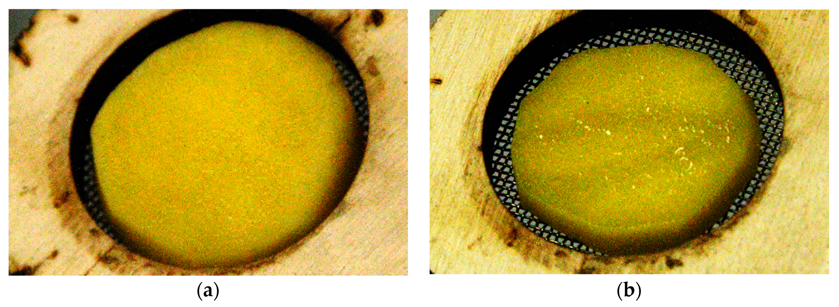
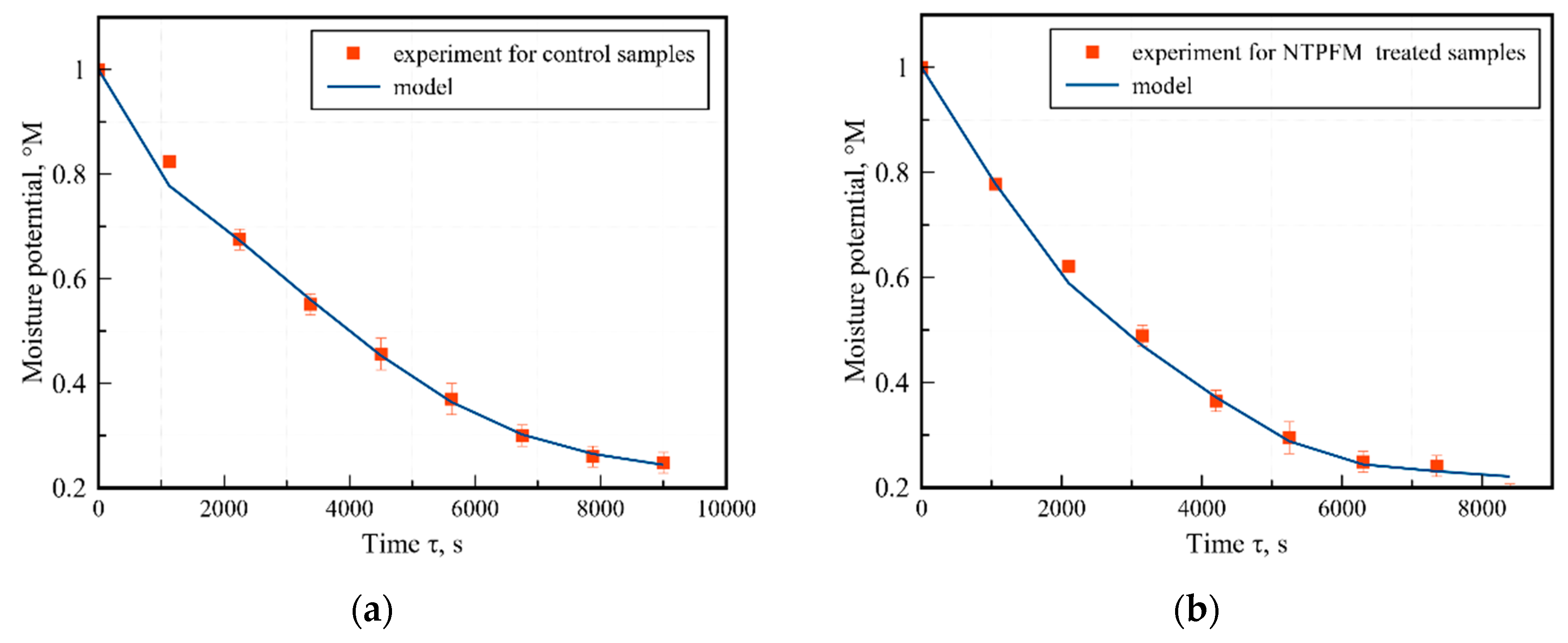
4.2. Experimental Results

The sample surface of the intact (Figure 2a) and NTPFM pretreated samples (Figure 2b) are presented in Figure 2. Obtained NTPFM treatment induces electrical breakdown or a disruption of the biological membrane. The membrane disruption by NTPFM treatment will affect the drying characteristics of potato samples by increasing the mass transfer of water. NTPFM treatments were conducted by 5 kV/cm using a fixed pulse width of 30 µs and a pulse frequency of 100 Hz assisted by thermionic emission. NTPFM treatment time was 120 s. The effects of the NTPFM treatments on the moisture ratio of potato samples are shown in Figure 3. The drying of the intact samples, until moisture ratio 0.05, lasted 152 min, whereas for the NTPFM-treated samples it took 126 min. It means that the NTPFM application reduced the process time by 20.6% in comparison to the control sample.

Further work will be done to explain the mechanism of NTPFM on material tissue with textural measurement analysis, different electrical parameters variation and product quality.

4.3. Results of Numerical Modelling

A comparison of the experimental drying curve with a model from Equation (24) for NTPFM-treated and control samples is shown on Figure 4. Competently settled mathematical model allows for the prediction of the progress of the process. It can also be a helpful instrument for food technologists in making in terms of the necessary drying time and process optimization.

In our study, the mathematical modeling demonstrated that proposed model fit very well to the empirical data (discrepancy less than 3%). Kinetic coefficients from Equation (28) were used to find temperature and pressure potentials for NTPFM-treated and control samples. Figure 5a shows temperature potential curves for the potato sample. For the NTPFM-treated samples, a temperature drop at the initial time was observed (Figure 5a). This effect can be explained by cooling the sample surface with intracellular fluid, as explained in our previous work [3]. Turgor pressure reduction as a result of channel formation in the material by the NTPFM treatment affected the pressure potential curve. Thus, in samples previously treated by NTPFM, a lower pressure potential formed (Figure 5b).

A set of three nonlinear differential equations allowed for temperature and pressure fields to be obtained, which were not observed in an experiment. At the same time, the importance of assessment of the temperature field in practice is emphasized with a regulation of the process of carbonization and denaturation mode during the drying of agricultural materials. A pressure field promotes the possibility of the process of the material cracking to be adjusted, as well as the control of the mechanical durability of finished goods. Further work will be aimed at a detailed study of the processes arising from the NTPFM treatment of biomaterials.

5. Conclusions

Basing on Lykov theory of heat, mass and pressure transfer, a modified set of three differential equations in partial derivatives was obtained and proposed as a model for NTPFM treatment impact analysis, with the working variables of temperature, moisture and pressure. The finite element model was applied for the prediction of temperature, moisture and pressure variation during drying of NTPFM-treated and nontreated potato samples, and the model predicted the results with the experimental data. The solution of an optimization problem allowed for the specified values of kinetic coefficients from the drying curve to be received. The agreement of the simulation data with the analytical equation and experimental results is satisfactory (discrepancy less than 3%). From an experimental point of view, NTPFM application reduced the process time by 20.6% in comparison to the control sample. The obtained methodology, with its high accuracy (divergence less than 1%), can be used for biomaterial drying process analysis and to explain the effects after nonthermal pulsed filamentary microplasma treatment. Thus, from the data, only for one variable (be it from temperature, moisture or pressure), it is possible to recover the missing two variables and to perform optimization of the values of kinetic coefficients, with a possible explanation of the arising effects in the course of drying with a NTPFM pretreatment.

References

1. Traffano-Schiffo, M.V.; Tylewicz, U.; Castro-Giraldez, M.; Fito, P.J.; Ragni, L.; Dalla Rosa, M. Effect of pulsed electric fields pre-treatment on mass transport during the osmotic dehydration of organic kiwifruit. Innov. Food Sci. Emerg. Technol. 2016, 38, 243–251. [Google Scholar] [CrossRef]
2. Smith, K.C.; Weaver, J.C. Electrodiffusion of molecules in aqueous media: A robust, discretized description for electroporation and other transport phenomena. IEEE Trans. Biomed. Eng. 2012, 59, 1514–1522. [Google Scholar] [CrossRef] [PubMed]
3. Granot, Y.; Rubinsky, B. Mass transfer model for drug delivery in tissue cells with reversible electroporation. Int. J. Heat Mass Transf. 2008, 51, 5610–5616. [Google Scholar] [CrossRef] [PubMed]
4. Shorstkii, I.A. Evaluation of the effect of a pulsed electric discharge on the process of substance transfer in plant material at the initial moment of time. Universities proceedings. Food Technol. 2019, 2, 73–77. [Google Scholar]
5. Shorstkii, I.A.; Khudykov, D.A. Pulsed electric field pre-treatment efficiency analysis in processes of biomaterials drying. Vestnik VGUIT [Proc. VSUET] 2018, 80, 49–54. [Google Scholar] [CrossRef]
6. Wiktor, A.; Śledź, M.; Małgorzata, N.; Chudoba, T.; Witrowa-Rajchert, D. Pulsed Electric Field Pretreatment for Osmotic Dehydration of Apple Tissue: Experimental and Mathematical Modeling Studies. Dry. Technol. Int. J. 2014, 32, 408–417. [Google Scholar] [CrossRef]
7. Mahnič-Kalamiza, S.; Vorobiev, E. Dual-porosity model of liquid extraction by pressing from biological tissue modified by electroporation. J. Food Eng. 2014, 137, 76–87. [Google Scholar] [CrossRef]
8. Parniakov, O.; Bals, O.; Lebovka, N.; Vorobiev, E. Pulsed electric field assisted vacuum freeze-drying of apple tissue. Innov. Food Sci. Emerg. Technol. 2016, 35, 52–57. [Google Scholar] [CrossRef]
9. Won, Y.C.; Min, S.C.; Lee, D.U. Accelerated Drying and Improved Color Properties of Red Pepper by Pretreatment of Pulsed Electric Fields. Dry. Technol. Int. J. 2015, 33, 926–932. [Google Scholar] [CrossRef]
10. Pavlin, M.; Miklavcic, D. Theoretical and experimental analysis of conductivity, ion 1285 diffusion and molecular transport during cell electroporation—Relation between short-lived and long-lived pores. Bioelectrochemistry 2008, 74, 38–46. [Google Scholar] [CrossRef] [PubMed]
11. Bouzrara, H.; Vorobiev, E. Solid-liquid expression of cellular materials enhanced by pulsed electric field. Chem. Eng. Process. 2003, 42, 249–257. [Google Scholar] [CrossRef]
12. Lebovka, N.I.; Shynkaryk, N.V.; Vorobiev, E. Pulsed electric field enhanced drying of potato tissue. J. Food Eng. 2007, 78, 606–613. [Google Scholar] [CrossRef]
13. Liu, C.; Grimi, N.; Lebovka, N.; Vorobiev, E. Convective air, microwave, and combined drying of potato pre-treated by pulsed electric fields. Dry. Technol. 2018, 1–10. [Google Scholar] [CrossRef]
14. Zhang, X.L.; Zhong, C.S.; Mujumdar, A.S.; Yang, X.H.; Deng, L.Z.; Wang, J.; Xiao, H.W. Cold plasma pretreatment enhances drying kinetics and quality attributes of chili pepper (Capsicum annuum L.). J. Food Eng. 2019, 241, 51–57. [Google Scholar] [CrossRef]
15. Li, S.; Chen, S.; Han, F.; Xv, Y.; Sun, H.; Ma, Z.; Chen, J.; Wu, W. Development and Optimization of Cold Plasma Pretreatment for Drying on Corn Kernels. J. Food Sci. 2019, 84, 2181–2189. [Google Scholar] [CrossRef] [PubMed]
16. Khan, M.I.H.; Wellard, R.M.; Nagy, S.A.; Joardder, M.U.H.; Karim, M.A. Experimental investigation of bound and free water transport process during drying of hygroscopic food material. Int. J. Therm. Sci. 2017, 117, 266–273. [Google Scholar] [CrossRef]
17. Kudra, T.; Martynenko, A. Electrohydrodynamic drying: Theory and experimental validation. Dry. Technol. 2019. [Google Scholar] [CrossRef]
18. Lykov, A.V. Drying Theory; Energiya: Moscow, Russia, 1968. [Google Scholar]
19. Kamangar, T.; Farsam, H. Composition of pistachio kernels of various Iranian origins. J. Food Sci. 1997, 42, 135–136. [Google Scholar] [CrossRef]
20. Shorstkii, I.; Mirshekarloo, M.S.; Koshevoi, E. Application of Pulsed Electric Field for Oil Extraction from Sunflower Seeds: Electrical Parameter Effects on Oil Yield. J. Food Process Eng. 2017, 40, e12281. [Google Scholar] [CrossRef]
21. Lykov, A.V.; Mihailov, Y.A. Heat and Mass Transfer Theory; Energiya: Moscow, Russia, 1963. [Google Scholar]
22. Ginzburg, A.S. Thermophysical Characteristics of Foodstuffs and Food Materials; Food Industry: Moscow, Russia, 1975. [Google Scholar]
23. Wu, Y. Effect of Pressure on Heat and Mass Transfer in Starch-based Food Systems. Ph.D. Thesis, University of Saskatchewan, Saskatoon, SK, Canada, 1997. [Google Scholar]
24. Tsukada, T.; Sakai, N.; Hayakawa, K. Computerised model for strain-stress analysis of food undergoing simultaneous heat and mass transfer. J. Food Sci. 1991, 56, 1438–1445. [Google Scholar] [CrossRef]
25. Nikitina, L.M. Thermodynamic Parameters and Mass Transfer Coefficients in Moist Materials; Energiya: Moscow, Russia, 1968. [Google Scholar]
26. Barron, R.F.; Nellis, G.F. Cryogenic Heat Transfer, 2nd ed.; CRC Press: Boca Raton, FL, USA, 2016. [Google Scholar] [CrossRef]
Figure 1. Experimental set-up used to provide nonthermal pulsed filamentary microplasma (NTPFM) treatment assisted by thermionic emission (TE) (a); schematic visualization of treatment trajectory in a treatment cell (not to scale) (b); and visualization of a NTPFM treatment process (c).
Chemengineering 03 00091 g001
Figure 2. Potato intact sample surface (a); and potato sample after NTPFM treatment with drops of liquid on the surface after PEF treatment (b) (not the same samples).
Chemengineering 03 00091 g002
Figure 3. The moisture ratio ω versus drying time τ for intact (control) and NTPFM-treated samples.
Chemengineering 03 00091 g003
Figure 4. The schedule of an average on thickness of value of moisture content over time, according to the model (the continuous line) and an experiment (marker) for control samples (a), and PEF-treated samples (b).
Chemengineering 03 00091 g004
Figure 5. Predicted temperature potential T (a) and pressure potential P (b) profile curves based on the specified kinetic coefficients for control and NTPFM-treated samples.
Chemengineering 03 00091 g005