Lattice-Boltzmann Simulation and Experimental Validation of a Microfluidic T-Junction for Slug Flow Generation


Abstract
1. Introduction
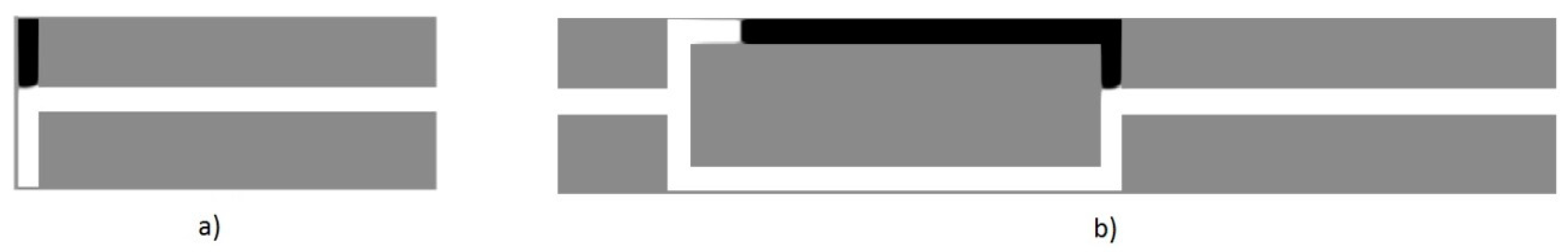
1.1. Geometry
1.2. Contact Angle
1.3. Flow Rate
1.4. Viscosity
1.5. Surface Tension
2. Materials and Methods
2.1. Multiphase LBM
2.2. Rothman and Keller or Color Gradient Model
2.3. Single-Phase Collision
2.4. Collision or Perturbation Operator
2.5. Two-Phase Collision (Recoloring)
3. Model Implementation and Hardware Requirements
4. Model validation
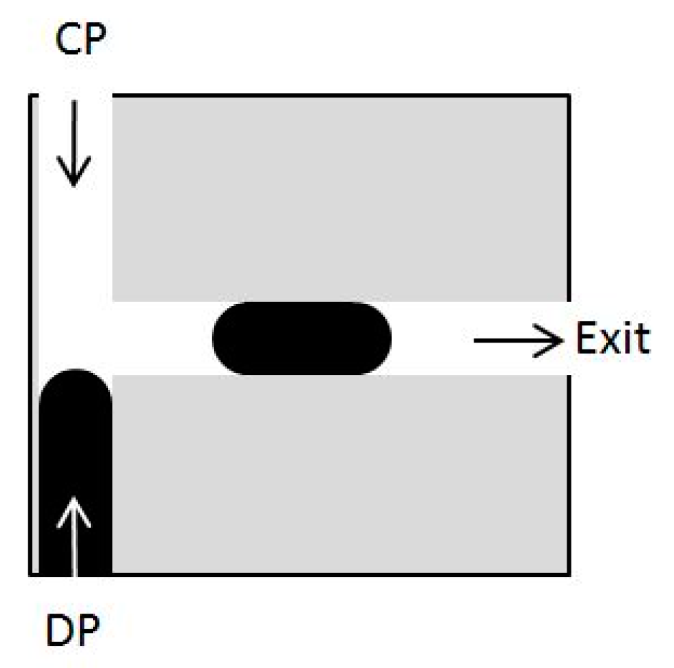
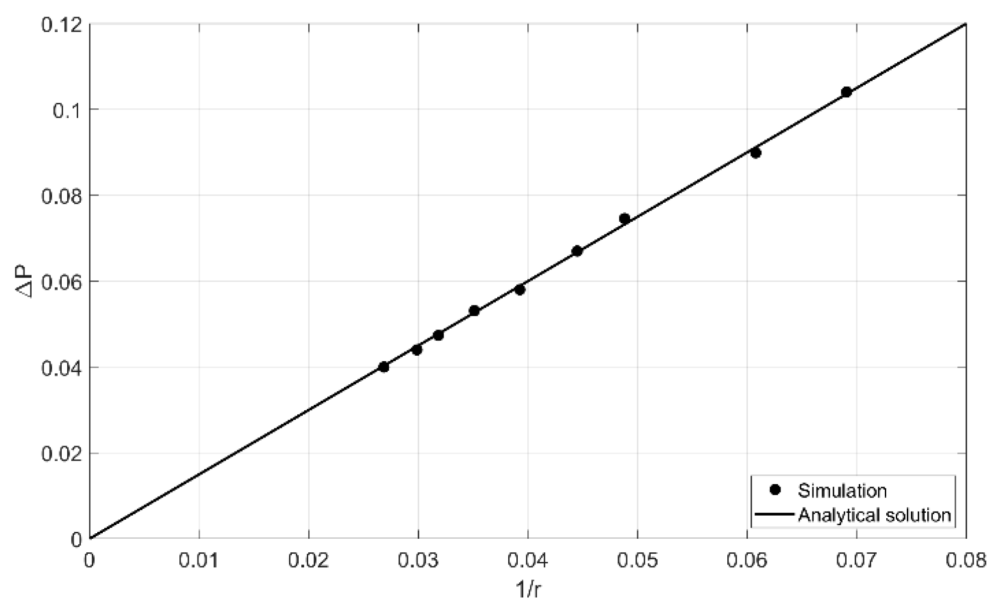
4.1. Laplace Test
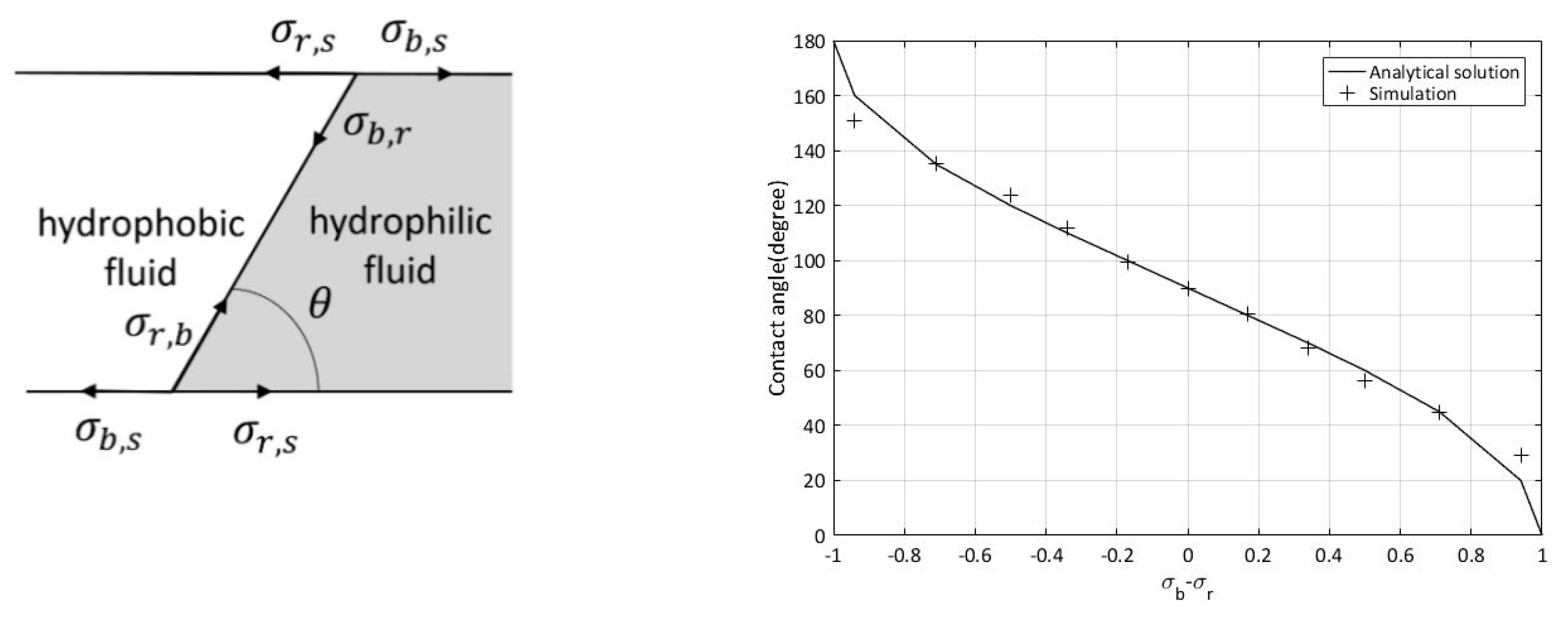
4.2. Static Contact Angle
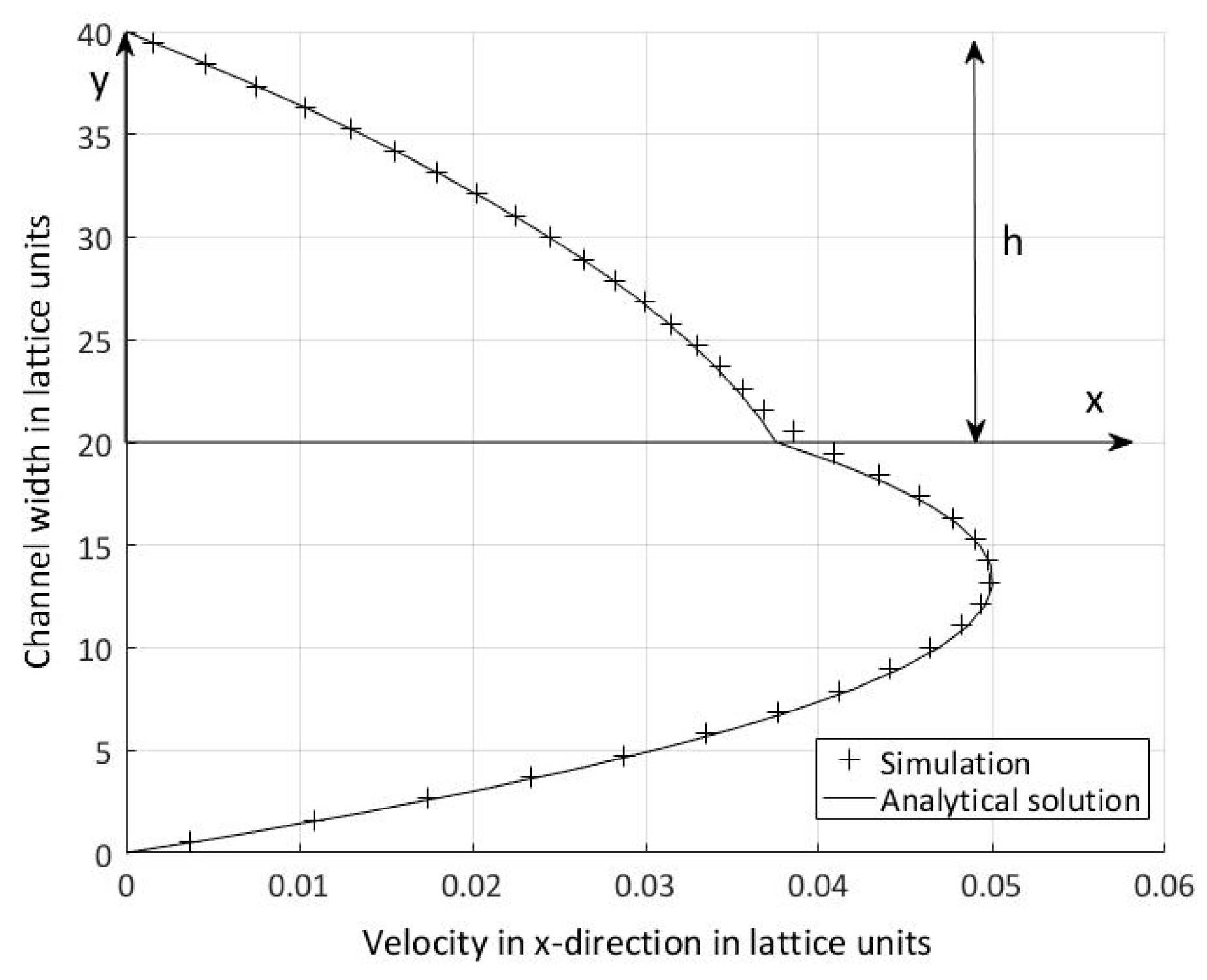
4.3. Layered Flow for Immiscible Two-Phase Flow
5. Results
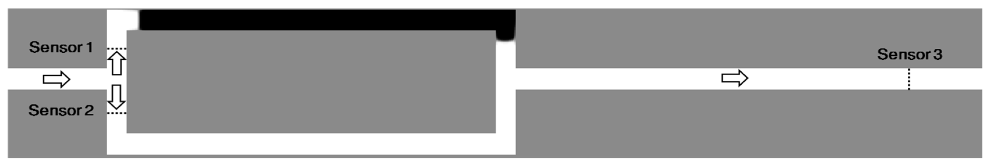
5.1. Simulation of the Droplet Formation in the Head-On Device
5.2. Velocity-Pressure Boundary Conditions
5.3. Periodic Boundary Conditions and Volume Force
5.4. Flow Conditions
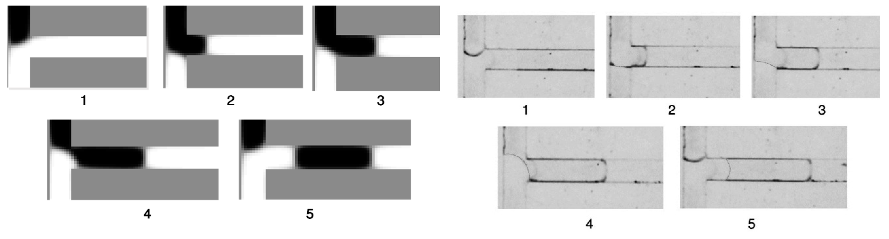
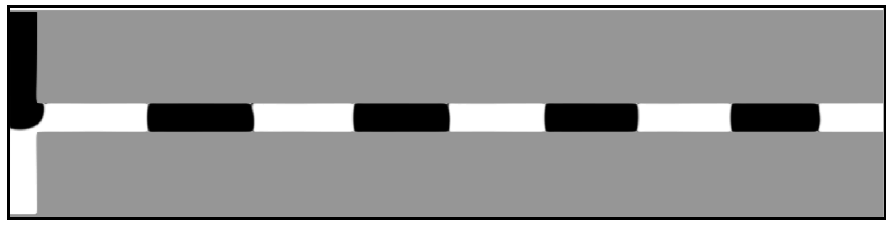
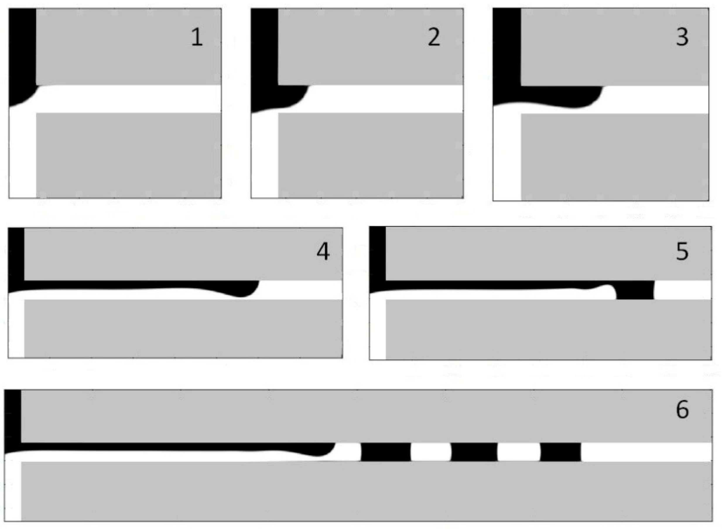
5.5. Droplet Formation Process
5.6. Dripping-Squeezing
5.7. Jetting-Shearing
5.8. Threading
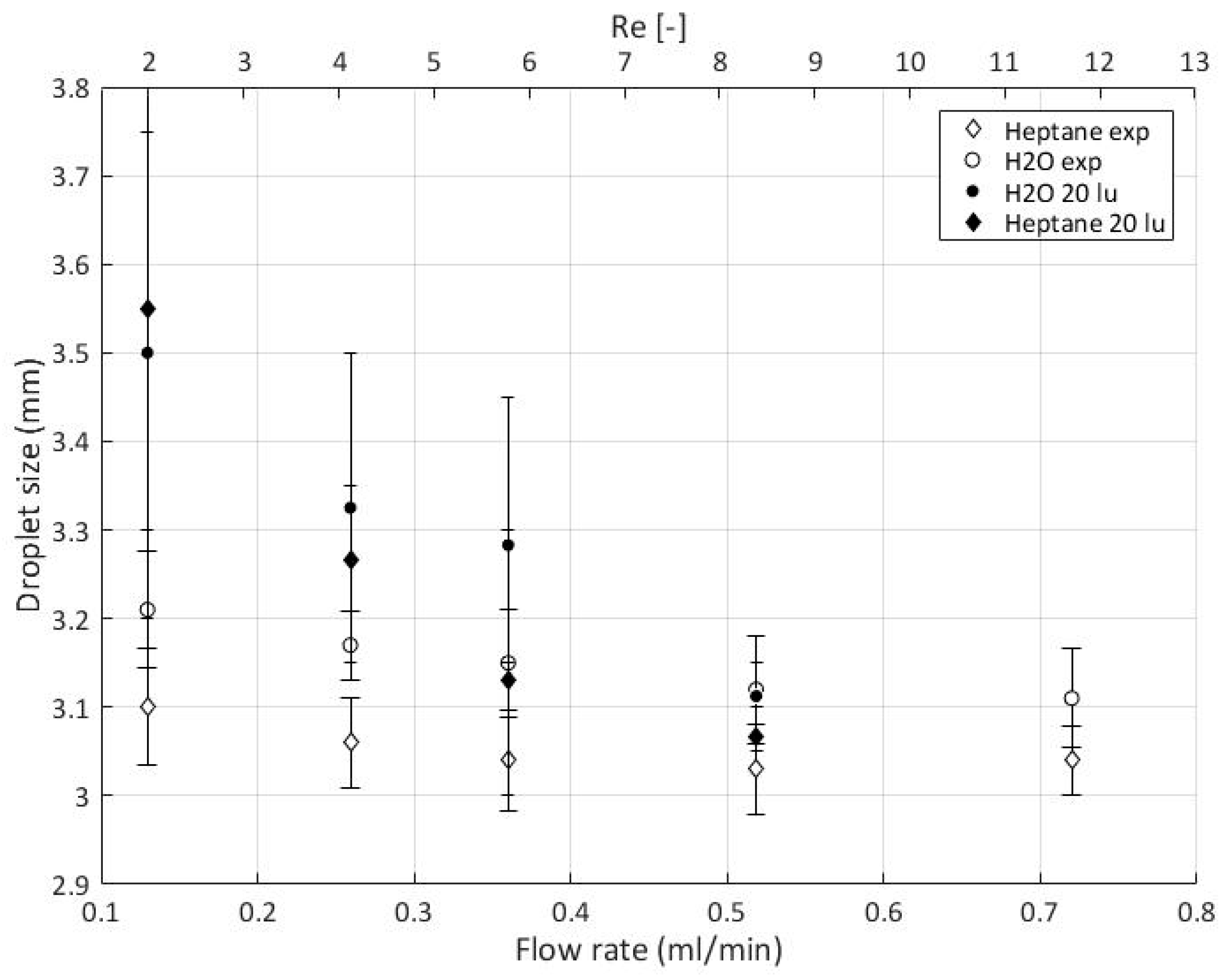
5.9. Experimental Data
6. Discussion
Quantitative Comparison between Simulation and Experimental Data
7. Conclusions
Author Contributions
Funding
Conflicts of Interest
References
- Bashir, S.; Rees, J.M.; Zimmerman, W.B. Simulations of microfluidic droplet formation using the two-phase level set method. Chem. Eng. Sci. 2011, 66, 4733–4741. [Google Scholar] [CrossRef]
- Li, X.-B.; Li, F.-C.; Yang, J.-C.; Kinoshita, H.; Oishi, M.; Oshima, M. Study on the mechanism of droplet formation in T-junction microchannel. Chem. Eng. Sci. 2012, 69, 340–351. [Google Scholar] [CrossRef]
- Song, H.; Chen, D.L.; Ismagilov, R.F. Reactions in Droplets in Microfluidic Channels. Angew. Chem. Int. Ed. 2006, 45, 7336–7356. [Google Scholar] [CrossRef] [PubMed]
- Yan, Y.; Guo, D.; Wen, S. Numerical simulation of junction point pressure during droplet formation in a microfluidic T-junction Chemical. Eng. Sci. 2012, 24, 591–601. [Google Scholar] [CrossRef]
- Gu, H.; Duits, M.H.G.; Mugele, F. Droplets Formation and Merging in Two-Phase Flow Microfluidics. Int. J. Mol. Sci. 2011, 12, 2572–2597. [Google Scholar] [CrossRef] [PubMed]
- Glawdel, T.; Elbuken, C.; Ren, C.L. Droplet formation in microfluidic T-junction generators operating in the transitional regime. I. Experimental observations. Phys. Rev. E 2012, 85, 016322. [Google Scholar] [CrossRef]
- Garstecki, P.; Fuerstman, M.J.; Stone, H.A.; Whitesides, G.M. Formation of droplets and bubbles in a microfluidic T-junction scaling and mechanism of break-up. Lab Chip 2006, 6, 437–446. [Google Scholar] [CrossRef]
- O’Brien, M.; Cooper, D.A.; Dolan, J. Continuous flow iodination using an automated computer-vision controlled liquid-liquid extraction system. Tetrahedron Lett. 2017, 58, 829–834. [Google Scholar] [CrossRef][Green Version]
- O’Brien, M.; Koos, P.; Browne, D.L.; Ley, S.V. A prototype continuous-flow liquid–liquid extraction system using open-source technology. Org. Biomol. Chem. 2012, 10, 7031. [Google Scholar] [CrossRef]
- Kaske, F.; Dick, S.; Pajoohi, S.A.; Agar, D.W. The influence of operating conditions on the mass transfer performance of a micro capillary contactor with liquid–liquid slug flow. Chem. Eng. Process. Process Intensif. 2016, 108, 10–16. [Google Scholar] [CrossRef]
- Hessel, V.; Kralisch, D.; Kockmann, T.N.; Wang, Q. Novel Process Windows for Enabling, Accelerating, and Uplifting Flow Chemistry. ChemSusChem 2013, 6, 746–789. [Google Scholar] [CrossRef]
- Gutmann, B.; Cantillo, D.; Kappe, C.O. Kontinuierliche Durchflussverfahren: Ein Werkzeug für die sichere Synthese von pharmazeutischen Wirkstoffen. Angew. Chem. 2015, 127, 6788–6832. [Google Scholar] [CrossRef]
- Gutmann, B.; Cantillo, D.; Kappe, C.O. Continuous-Flow Technology-A Tool for the Safe Manufacturing of Active Pharmaceutical Ingredients. Angew. Chem. Int. Ed. 2015, 54, 6688–6728. [Google Scholar]
- Terao, K.; Nishiyama, Y.; Kakiuchi, K. Highly Efficient Asymmetric Paternò—Büchi Reaction in a Microcapillary Reactor Utilizing Slug Flow. J. Flow Chem. 2014, 4, 35–39. [Google Scholar] [CrossRef]
- Colosqui, C.E.; Cheah, M.J.; Kevrekidis, I.G.; Benziger, J.B. Droplet and slug formation in polymer electrolyte membrane fuel cell flow channels: The role of interfacial forces. J. Power Sources 2011, 196, 10057–10068. [Google Scholar] [CrossRef]
- Gemoets, H.P.L.; Su, Y.; Shang, M.; Hessel, V.; Luqueb, R.; Noël, T. Liquid phase oxidation chemistry in continuous-flow microreactors. Chem. Soc. Rev. 2016, 45, 83–117. [Google Scholar] [CrossRef] [PubMed]
- Baumeister, T.; Kitzler, H.; Obermaier, K.; Zikeli, S.; Röder, T. Two-Phase Flow Oxidation of Valeraldehyde with O2 in a Microstructured Reactor. Process Res. Dev. 2015, 19, 1576–1579. [Google Scholar] [CrossRef]
- Borukhova, S.; Noël, T.; Hessel, V. Hydrogen Chloride Gas in Solvent-Free Continuous Conversion of Alcohols to Chlorides in Microflow Org. Process Res. Dev. 2016, 20, 568–573. [Google Scholar] [CrossRef]
- Matthias, M.; Nachtrodt, H.; Mescher, A.; Ghaini, A.; Agar, D.W. Design and Control Techniques for the Numbering-up of Capillary Microreactors with Uniform Multiphase Flow Distribution. Ind. Eng. Chem. Res. 2010, 49, 10908–10916. [Google Scholar]
- Shi, Y.; Tang, G.; Xia, H. Lattice Boltzmann simulation of droplet formation in T-junction and flow focusing devices. Comput. Fluids 2014, 90, 155–163. [Google Scholar] [CrossRef]
- Liu, H.; Zhang, Y. Droplet formation in a T-shaped microfluidic junction. J. Appl. Phys. 2009, 106, 034906. [Google Scholar] [CrossRef]
- De Menech, M.; Garstecki, P.; Jousse, F.; Stone, H.A. Transition from squeezing to dripping in a microfluidic T-shaped junction. J. Fluid Mech. 2008, 595, 141–161. [Google Scholar] [CrossRef]
- Gupta, A.; Murshed, S.M.S.; Kumar, R. Droplet formation and stability of flows in a microfluidic T-junction. Appl. Phys. Lett. 2009, 94, 164107. [Google Scholar] [CrossRef]
- Bashir, S.; Bashir, M.; Solvas, X.; Rees, J.; Zimmmerman, W. Hydrophilic Surface Modification of PDMS Microchannel for O/W and W/O/W Emulsions. Micromachines 2015, 6, 1445–1458. [Google Scholar] [CrossRef]
- Van der Graaf, S.; Nisisako, T.; Schroën, C.G.; van der Sman, R.G.; Boom, R.M. Lattice Boltzmann simulations of droplet formation in a T-shaped microchannel. Langmuir 2006, 22, 4144–4152. [Google Scholar] [CrossRef] [PubMed]
- Leclaire, S.; Reggio, M.; Trépanier, J.-Y. Isotropic color gradient for simulating very high-density ratios with a two-phase flow lattice Boltzmann model. Comput. Fluids 2011, 48, 98–112. [Google Scholar] [CrossRef]
- Leclaire, S.; Reggio, M.; Trépanier, J.-Y. Numerical evaluation of two recoloring operators for an immiscible two-phase flow lattice Boltzmann model Modelling. Appl. Math. 2012, 36, 2237–2252. [Google Scholar]
- Leclaire, S.; Reggio, M.; Trépanier, J.-Y. Progress and investigation on lattice Boltzmann modeling of multiple immiscible fluids or components with variable density and viscosity ratios. J. Comput. Phys. 2013, 246, 318–342. [Google Scholar] [CrossRef]
- Danner, T.; Eswara, S.; Schulz, V.P.; Latz, A. Characterization of gas diffusion electrodes for metal-air batteries. J. Power Sources 2016, 324, 646–656. [Google Scholar] [CrossRef]
- Reis, T.; Phillips, T.N. Lattice Boltzmann model for simulating immiscible two-phase flows. J. Phys. A Math. Theor. 2007, 40, 4033. [Google Scholar] [CrossRef]
- Latva-Kokko, M.; Rothman, D.H. Diffusion properties of gradient-based lattice Boltzmann models of immiscible fluids. Phys. Rev. 2005, 71, 056702. [Google Scholar] [CrossRef] [PubMed]
- Huang, H.; Sukop, M.; Lu, X. Multiphase Lattice Boltzmann Methods: Theory and Application; John Wiley & Sons: Hoboken, NJ, USA, 2015. [Google Scholar]
- Laplace, P.S. Traité de Mécanique Céleste 4; l’Imprimerie de Crapelet: Paris, France, 1805. [Google Scholar]
- Tölke, J. Gitter-Boltzmann-Verfahren zur Simulation von Zweiphasenströmungen; Shaker: München, Germany, 2001; pp. 54–56. [Google Scholar]
- Sukop, M.C.; Thorne, D.T. An Introduction for Geoscientists; Springer: Berlin/Heidelberg, Germany, 2006; p. 60. [Google Scholar]
- Krueger, T. Computer Simulation Study of Collective Phenomena in Dense Suspensions of Red Blood Cells under Shear, 1st ed.; Springer Spektrum: Berlin, Germany, 2012; pp. 27–28. [Google Scholar]
- Thorsen, T.; Roberts, R.W.; Arnold, F.H.; Quake, S.R. Dynamic Pattern Formation in a Vesicle-Generating Microfluidic Device. Phys. Rev. Lett. 2001, 86, 4163–4166. [Google Scholar] [CrossRef] [PubMed]
- Shui, L.; van den Berg, A.; Eijkel, J.C.T. Capillary instability, squeezing, and shearing in head-on microfluidic. J. Appl. Phys. 2009, 106, 124305. [Google Scholar] [CrossRef]
- Shui, L. Two-Phase Flow in Micro and Nanofluidic Devices; Twente, U.O., Ed.; Wohrmann Print Service: Zutphen, The Netherlands; Enschede, The Netherlands, 2009. [Google Scholar]


| Parameter | Dimension | Simulation | Experiment |
|---|---|---|---|
| Channel width | (mm) | 10, 20, 40 a lu ≈ 1 mm | 1 |
| Viscosity ratio | (mm) | 0.6839 | 0.6839 |
| Density ratio | (mm) | 1 | 1.468 |
| Contact angle | (°) | 80 | About 90 |
| Ratio of volume | (-) | 1 | 1 |
| Reynolds number | (-) | 2–9 | 2–12 |
| Capillary number | (-) | 10−3–10−1 | 10−5–10−4 |
| Flow rate | (mL/min) | 0.13–0.58 | 0.13–0.72 |
© 2019 by the authors. Licensee MDPI, Basel, Switzerland. This article is an open access article distributed under the terms and conditions of the Creative Commons Attribution (CC BY) license (http://creativecommons.org/licenses/by/4.0/).
Share and Cite
Schulz, V.P.; Abbaspour, N.; Baumeister, T.; Röder, T. Lattice-Boltzmann Simulation and Experimental Validation of a Microfluidic T-Junction for Slug Flow Generation. ChemEngineering 2019, 3, 48. https://doi.org/10.3390/chemengineering3020048
Schulz VP, Abbaspour N, Baumeister T, Röder T. Lattice-Boltzmann Simulation and Experimental Validation of a Microfluidic T-Junction for Slug Flow Generation. ChemEngineering. 2019; 3(2):48. https://doi.org/10.3390/chemengineering3020048
Chicago/Turabian StyleSchulz, Volker Paul, Nima Abbaspour, Tobias Baumeister, and Thorsten Röder. 2019. "Lattice-Boltzmann Simulation and Experimental Validation of a Microfluidic T-Junction for Slug Flow Generation" ChemEngineering 3, no. 2: 48. https://doi.org/10.3390/chemengineering3020048
APA StyleSchulz, V. P., Abbaspour, N., Baumeister, T., & Röder, T. (2019). Lattice-Boltzmann Simulation and Experimental Validation of a Microfluidic T-Junction for Slug Flow Generation. ChemEngineering, 3(2), 48. https://doi.org/10.3390/chemengineering3020048