Robust Initialization of Rigorous Process Simulations of Multiple Dividing Wall Columns via V_min Diagrams

Abstract

Dividing Wall Columns (DWCs) allow the separation of a ternary mixture in one column shell by applying a vertical partition wall, yielding a reduction of operational and capital costs of up to 30%. Multiple DWC (mDWC), the consequent advancement of standard DWC, makes use of more than one partitioning wall, allowing the separation of quaternary or even higher mixtures in one column shell accompanied by a further reduction of energy consumption. Since no dedicated models for these columns are available in commercial process simulators, thermodynamic consistent flowsheets have to be designed and implemented. The thermally fully coupled Petlyuk arrangement is one important example. However, the initial convergence of these substituting flowsheets is demanding, since a large number of meaningful initial guesses have to be provided. A promising method for generating these first estimates are minimum vapor (V_min) diagrams. All internal flows can be extracted from these diagrams and used for robust initialization of the simulation. The goal of this work is to present the V_min method in a comprehensive way in order to initialize mDWC simulations to predict the separation of four component mixtures. Additionally, the adaptation of the diagram to configurations different than Petlyuk arrangements for mDWC is evaluated and a systematic procedure to obtain them is presented. In the end, an example of a converging simulation is given, which was obtained with the values from the V_min diagram.

1. Introduction

Distillation captures a large amount of energy consumption in chemical processes. A typical example of an intensified process offering the opportunity to reduce this energy demand are Dividing Wall Columns (DWCs). Conventionally, the separation of a ternary mixture via distillation is performed in a sequence of two distillation columns, each having its own reboiler and condenser. To reduce the investment costs and space, the process can be combined in one column shell with a side draw for the intermediate boiling component. Nevertheless, this does not lead to a pure side product since the feed remixes with the product stream. This can be avoided by using a dividing wall in the middle of the column, which prevents backmixing, resulting in a reduction of operational costs [1,2,3]. Extending this method results in multiple Dividing Wall Columns (mDWC) which are able to separate multicomponent mixtures in one column shell [4]. This work focuses on mDWC for the separation of a four component feed mixture. 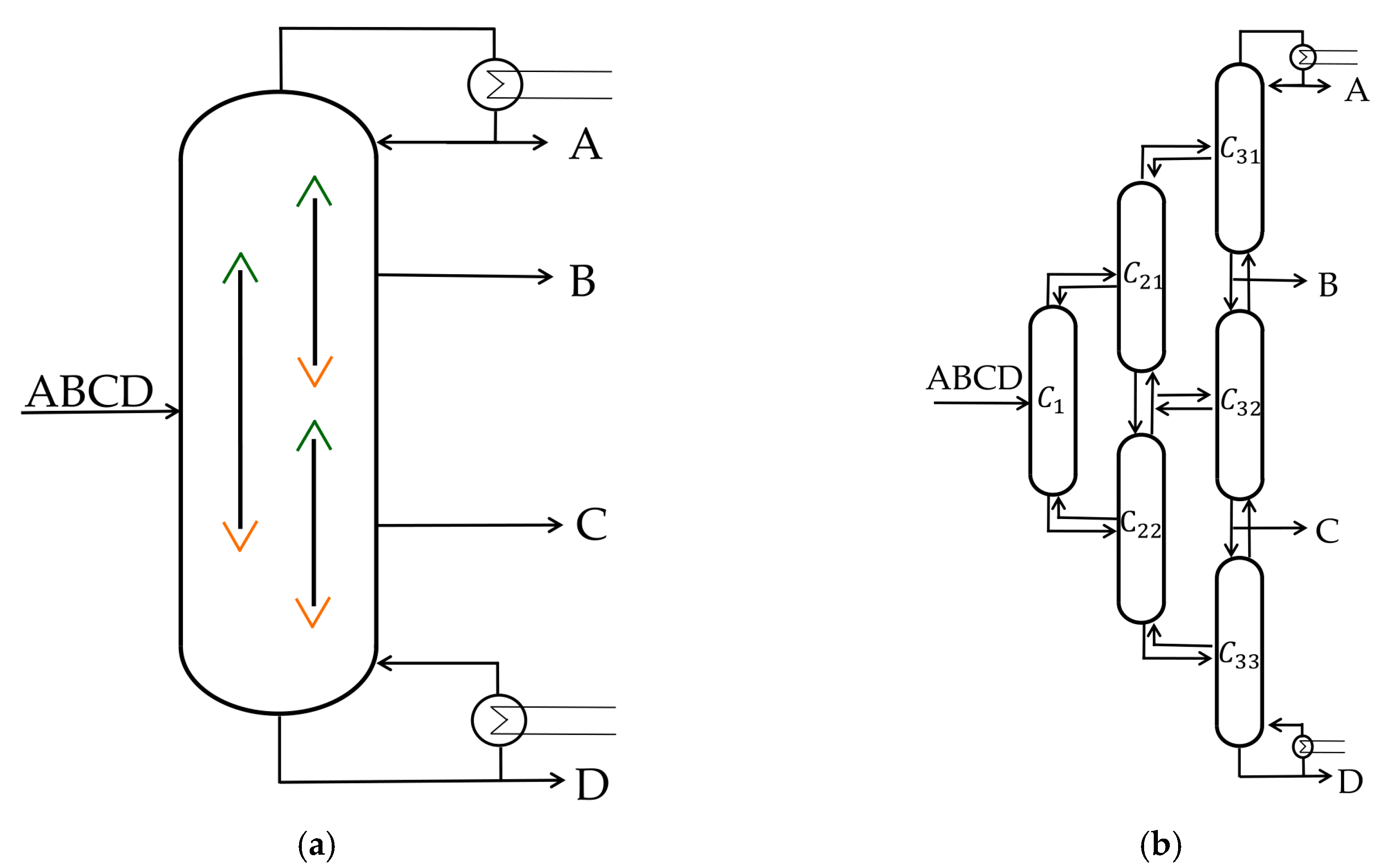Figure 1a shows a typical four product Dividing Wall Column with three dividing walls.

The intensification results in a higher number of degrees of freedom for mDWC compared to the conventional separation, including liquid and vapor splits at each dividing wall, as indicated as green and orange lines in Figure 1a. The liquid and vapor splits distribute the internal streams in a way that enables ideal product splits in each column section. This results in a high complexity of mDWCs, which is the reason why none have been built yet.

For the design of mDWC, computer-based rigorous simulations are indispensable [5]. Even though there are no default models in process simulators available for Dividing Wall Columns with more than one dividing wall, there are methods to implement these that result in a thermodynamically consistent flowsheet. Among other things [2], different sections of the column can be implemented as a sequence of fully thermally coupled columns, also called the Petlyuk sequence [6]. Fully thermally coupled columns are interconnected via vapor and liquid streams. In the case of a Petlyuk sequence, only one reboiler and one condenser is present, as shown in Figure 1b. The shown Petlyuk sequence is thermally equivalent to the mDWC in Figure 1a. Note that the first column in the sequence C₁ will be called the prefractionator in the following text. In order to reduce the complexity, the number and configuration of the dividing walls can be changed. This results in equivalent thermally coupled column sequences different to the Petlyuk sequence. An example of a four product DWC with a reduced number of splits is the Kaibel column [7], which will be presented later in Section 4.2. The corresponding column sequence consists of only three thermodynamically coupled columns compared to six for the conventional Petlyuk sequence.

The main challenge of the flowsheet simulation is to obtain meaningful initial estimations of coupling streams, since these are important when attempting to reach a converging simulation. A promising method to determine initial streams for a rigorous simulation is the V_min method [1] presented by Halvorsen and Skogestad [8,9,10] based on Underwood’s method [11]. V_min diagrams are obtained for only one column depicting different split cases. Nevertheless, they can also be applied for sequences of fully thermally coupled columns. Based on this, internal streams can be extracted and applied for the simulation initialization. In the literature, V_min diagrams are often only used to compare the minimum energy demand of different column sequences. In contrast to that, the V_min diagrams will be presented as an effective and robust tool to initialize rigorous simulations for the design of multiple Dividing Wall Columns.

This work comprehensively summarizes the publications of Halvorsen and Skogestadt [8,9,10] and Fidkowski and Agrawal [12], with a focus on mDWCs. Example calculations developed by the author of this paper shall help advance understanding of the method. The basic principles have to be comprehended in order to understand the main part of this work. These are changes of V_min diagrams caused by changes of thermal coupling in the column sequence. A publication of Ge et al. [13] also deals with this topic. However, only the final equations are presented without a detailed description of the calculation procedure. Hence, in this work, a systematic procedure is presented which can be performed to obtain V_min diagrams for differently thermally coupled columns. In the end, a V_min diagram will be applied to a practical example to initialize a rigorous simulation.

2. V_min Diagrams: Fundamentals

In a conventional distillation column, there are two degrees of freedom. This means that a plot of the feed-related vapor stream V/F over the feed-related distillate stream D/F results in a total description of the process. Since any combination of these streams is possible, it is more meaningful to determine the minimum vapor flow V_min that is necessary to obtain a certain product purity. For determining V_min, Underwoods method can be used [11], for which only the feed stream, its composition, and its liquid fraction have to be known. The resulting minimum vapor flow and the corresponding distillate stream are shown in the V_min diagram.

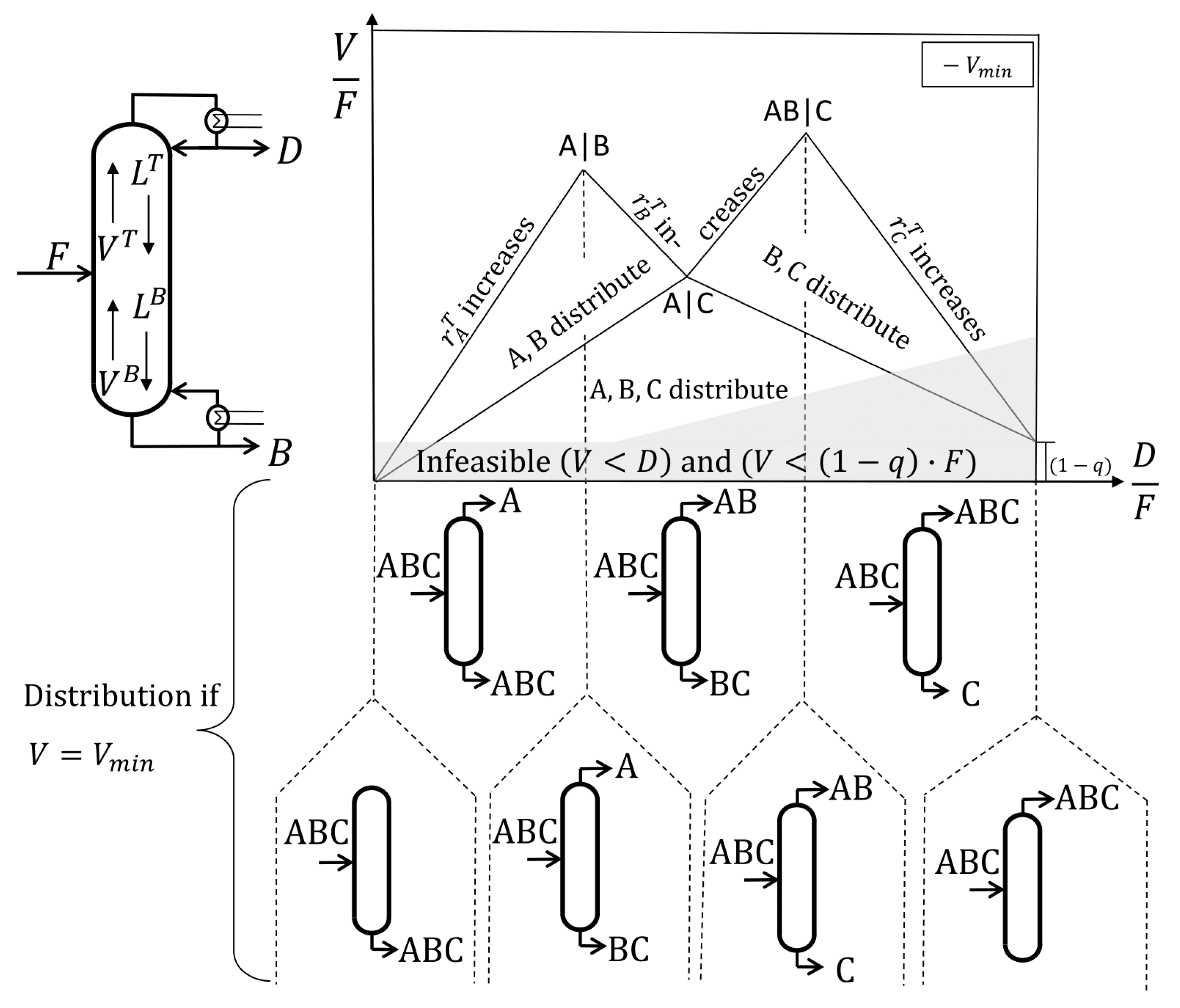
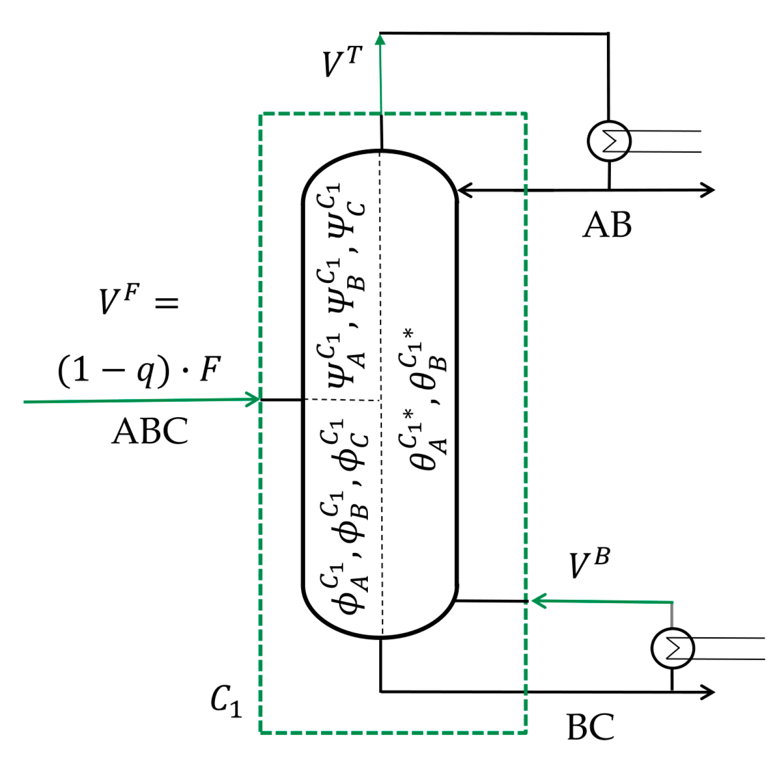
An example of a ternary mixture containing components ABC with A, the light boiler, and C, the heavy boiler, is given in Figure 2. The V_min diagram is obtained by the concept of a simple standard distillation column with an infinite number of stages. The recovery r describes the molar flow of a component in the distillate stream compared to the feed stream (see Equation (1)), having a value from zero to one. The corresponding recovery at the bottom of the column is calculated with the bottom stream.

$$r_i^T=\frac{D_i}{F_i}$$

(1)

The internal liquid flow L and vapor flow V are differentiated according to their location in the column, and the superscripts T and B indicate the corresponding recovery in the top (distillate) and the bottom stream of the column, respectively. This syntax was adopted from the publications of Halvorsen and Skogestad [8,9,10], who developed the method.

In any case, there are two infeasible regions indicated by the grey-shaded area in Figure 1. First, the vapor flow inside the column cannot be smaller than the amount of vapor in the feed stream, resulting in $V<\left(1-q\right)·F$ with q, the liquid fraction in the feed stream, to be infeasible. Second, there cannot be a higher distillate stream than vapor going up, which means that $V<D$ is infeasible. Having this in mind, the V_min line will be explained in the following. For a column without distillate stream, the minimum vapor flow would also be zero, and due to this, the diagram starts at (0|0). Increasing the distillate stream means increasing the recovery of the light boiler, which is component A in the top of the column. In order to get pure component A in the distillate without impurities, the minimum vapor flow shown in the diagram as a solid line is necessary. If less vapor is used, component B will also be in the distillate stream, and one says it distributes between the distillate and the bottom stream. Using more than the minimum vapor flow in a region above the V_min line is a waste of energy since the same product composition is reached even though more vapor is produced. Following the V_min line from the starting point (0|0), a straight line will be found on which the recovery of component A in the top of the column increases from zero to one. Reaching the recovery of one while the recoveries of the middle and heavy boiling components B and C are still zero is called a sharp split between A and B (A|B); in the following, it is written as the AB split. Sharp splits without a distributing component can be seen as maxima in the V_min diagram. Proceeding to higher D/F ratios also causes component B to be found in the distillate stream in addition to A, resulting in a decreasing minimum vapor flow. While the recovery of component B in the top of the column increases from zero to one, a minimum is passed. At that point, a sharp A|C, later denoted as AC, split at the minimum vapor demand is performed with component B distributing. For the ternary system, this split is called the preferred split of the prefractionator. A column works at the preferred split if it separates the lightest and the heaviest boiling components entering its feed stream at the corresponding minimum vapor flow. A further increase of the distillate stream after the AC split requires a higher minimum vapor flow for a distillate stream containing only component A and B. This means that the V_min line increases until the next maximum, the sharp AB|C split, is reached. Note that this split will result in the following be denoted as the BC split, even though component A is also considered to be in the top of the column. A further increase of the distillate streams means that also component C will move to the top product. This results in a decrease of the vapor flow demand. Nevertheless, this region is not meaningful for separation processes.

In summary:

• There are maxima and minima describing the vapor demand for sharp splits between the components
• For a multicomponent feed mixture (n = number of components) there are generally $\frac{n·\left(n-1\right)}{2}$ sharp splits, thereof $\left(n-1\right)$ without distributing component, $\left(n-2\right)$ with one distributing component etc. and $\frac{n·\left(n-1\right)}{2}+2$ significant points including:

  ○

  First boundary condition: no vapor results in no distillate $(0|0)$

  ○

  Second boundary condition: distillate is at least the vapor fraction of the feed $(1|1-q)$

• Infeasible region: $V<D$ and $V<\left(1-q\right)·F$
• Preferred split: Split between the lightest and heaviest component fed at the corresponding minimum vapor flow

3. Calculation of V_min Diagrams

V_min diagrams can be calculated by an analytical solution of the Underwood equations, which will be described in greater detail in the following chapter. First, the Underwood Roots will be briefly introduced in Section 3.1 and afterwards the analytical calculation is presented in Section 3.2. In the end, the significant steps used to calculate a V_min diagram of a four component mixture will be shown in Section 3.3.

3.1. Definition of Underwood Roots

The Underwood Roots are based on a mass balance around a simple distillation column with a feed stream at its middle, with the rectifying section above the feed stage and the stripping section below. An infinite number of stages, a constant molar flow, and constant relative volatilities of the components are assumed. The latter one is denoted as α_i, which is the distribution ratio of component i K_i compared to the distribution ratio of the overall heavy boiling component K_HB in the original feed mixture, as shown in Equation (2).

$${\alpha }_i=\frac{\raisebox{1ex}{$y_i$}\!\left/ \!\raisebox{-1ex}{$x_i$}\right.}{\raisebox{1ex}{$y_{HB}$}\!\left/ \!\raisebox{-1ex}{$x_{HB}$}\right.}=\frac{K_i}{K_{HB}}$$

(2)

where x_i, is the molar fraction of component i in the liquid phase and y_i, is the molar fraction of component i in the vapor phase. With these assumptions, Underwood [11] defined Equations (3) and (4) [14].

$${\displaystyle \sum }_i^n\frac{{\alpha }_i·x_i^T}{{\alpha }_i-\Phi }=R^T+1$$

(3)

$${\displaystyle \sum }_i^n\frac{{\alpha }_i·x_i^B}{{\alpha }_i-\Psi }=R^B$$

(4)

The superscript T indicates the top of the column and B is the bottom; accordingly, R^T is the reflux ratio, R^B is the boil up ratio, and Φ and Ψ are the Underwood Roots. There are different roots above and below the feed stage, which are called actual roots:

• Φ is the actual root in the rectifying section
• Ψ is the actual root in the stripping section

A pinch point analysis results in the following definitions for the actual roots: Equation (5) for the rectifying section and (6) for the stripping section [14].

$$\Phi =\frac{L^T}{V^T·K_{HB}}$$

(5)

$$\Psi =\frac{L^B}{V^B·K_{HB}}$$

(6)

L is the molar liquid stream and V the molar vapor stream. These internal streams differ depending on the performed product split. Hence, there are as many actual roots as components n in each section and their values are between the values of the relative volatilities of each component α_i (Equation (7)).

$$\begin{gathered} {\alpha }_1>{\Phi }_1>{\alpha }_2>{\Phi }_2>\dots >{\Phi }_n \\ {\Psi }_1>{\alpha }_1>{\Psi }_2>{\alpha }_2>\dots >{\alpha }_n \end{gathered}$$

(7)

A decreasing vapor flow results in increasing Ψ and decreasing Φ, which means that there is an intersection of the top and bottom roots. At this value, the minimum vapor flow V_min is reached and the roots are called common roots θ. There are n − 1 common roots fulfilling Equation (8).

$${\alpha }_1>{\Phi }_1={\Psi }_2={\theta }_1>{\alpha }_2\dots >{\alpha }_n$$

(8)

The common roots are called active roots ${\theta }^{*}$ if their value lies between the values of relative volatilities of the components, which are split as shown in Figure 3a. With $n_{dist}$, the number of distributing components (components with $r_i^T\ne 1$ or $0$) there is $n_{dist}+1$ active roots:

• For sharp splits (no distributing component), there is always only one active root, which is the one with a value between the volatilities of the components split
• For sharp splits with one distributing component, there are two active roots
• For sharp splits with two distributing components, there are three active roots etc.

Figure 3b symbolically shows all kinds of Underwood Roots in a distillation column for a sharp AC split with four components fed.

3.2. Analytical Calculation of V_min Diagrams

V_min diagrams are based on the Underwood Roots. The general calculation procedure is always the same, independent of the number of components. First, the Underwood Roots of the feed stream have to be calculated (Section 3.2.1). Second, in the case of sharp splits with distributing components, the recoveries of the distributing components have to be determined. If there are no splits with distributing components, this step is canceled. Third, the minimum vapor flow, as well as the distillate streams, can be calculated with the active roots and the recoveries (step 2 and 3 are presented in Section 3.2.2). Note that only the extreme points of the V_min diagram are calculated, which can be connected by straight lines. For a better understanding, the procedure is explained for a four component system in Section 3.2.3.

3.2.1. Calculation of the Common Roots

The common roots of the feed mixture are calculated with the first Underwood equation which is also called the feed equation (Equation (12)). In the following, the derivation of the equation is presented. First, a vapor flow balance around the column is performed, as shown in Figure 4.

Where F is the feed stream and V is the vapor stream; the superscripts B, T, and F indicate the streams at the bottom and top of the column and the feed stream, respectively; and q is the liquid fraction of the feed. The vapor balance results in Equation (9).

$$\left(1-q\right)·F+V^B=V^T$$

(9)

Based on the Underwood Roots, the vapor stream in the top of the column is defined by Equation (10) (for the derivation, see [15]).

$$V^T={\displaystyle \sum }_{i=1}^n\frac{{\alpha }_i·D_i}{{\alpha }_i-\Phi }={\displaystyle \sum }_{i=1}^n\frac{{\alpha }_i·F·z_i·r_i^T}{{\alpha }_i-\Phi }$$

(10)

D_i is the molar flow of component i in the distillate stream, z_i is the molar concentration of component i in the feed stream, and $r_i^T$ is the recovery of the component in the distillate stream (Equation (1)). The vapor flow in the bottom of the column is defined by Equation (11).

$$V^B={\displaystyle \sum }_{i=1}^n\frac{{\alpha }_i·B_i}{{\alpha }_i-\Psi }={\displaystyle \sum }_{i=1}^n\frac{{\alpha }_i·F·z_i·r_i^B}{{\alpha }_i-\Psi }$$

(11)

B_i is the molar flow of component i in the bottom stream and $r_i^B$ is the corresponding recovery related to the fed stream of the component. The minimum vapor flow is reached at $\Phi =\Psi =\theta$, with $r_i^B+r_i^T=1$. A combination of Equations (9)–(11) results in the so called feed equation, which is used to calculate the common roots (Equation (12)). Note that $r_i^B$ is defined for the outgoing bottom product, whereas the bottom vapor stream is incoming, which results in a negative sign that causes the recoveries to be canceled out.

$$V^F=\left(1-q\right)·F={\displaystyle \sum }_{i=1}^n\frac{{\alpha }_i·F·z_i}{{\alpha }_i-\theta }$$

(12)

3.2.2. Calculation of Minimum Vapor Flow

The second Underwood equation (Equation (13)) is used to calculate V_min depending on the active root ${\theta }^{*}$. Note that Equation (13) represents Equation (10) for the V_min case, meaning $\Phi =\theta$.

$$V_{min}={\displaystyle \sum }_{i=1}^n\frac{{\alpha }_i·D_i}{{\alpha }_i-{\theta }^{*}}={\displaystyle \sum }_{i=1}^n\frac{{\alpha }_i·z_i·F}{{\alpha }_i-{\theta }^{*}}·r_i^T$$

(13)

The index * means that only the active root of the split is used for the calculation. The corresponding distillate stream is calculated according to Equation (14).

$$D={\displaystyle \sum }_{i=1}^n{z}_i·r_i^T·F$$

(14)

The obtained data for V_min and D divided by the feed stream are plotted in the V_min diagram.

3.2.3. Example: V_min Diagram of a Four Component Feed

The relative volatilities of the feed components can be approximated manually by the extended Raoult’s Law, which is also implemented in simulation programs as Aspen HYSIS^®. There, the K-values of each component in the mixture can be read out and the relative volatilities α_i are determined with Equation (2). The common roots are calculated with Equation (12). Applying Equation (13) results in three equations that are needed to calculate the V_min diagram: Equation (15) for the first root A, Equation (16) for root B, and Equation (17) for root C.

$$\frac{V_{min}}{F}=\frac{{\alpha }_A·z_A}{{\alpha }_A-{\theta }_A^{*}}·r_A^T+\frac{{\alpha }_B·z_B}{{\alpha }_B-{\theta }_A^{*}}·r_B^T+\frac{{\alpha }_C·z_C}{{\alpha }_C-{\theta }_A^{*}}·r_C^T+\frac{{\alpha }_D·z_D}{{\alpha }_D-{\theta }_A^{*}}·r_D^T$$

(15)

$$\frac{V_{min}}{F}=\frac{{\alpha }_A·z_A}{{\alpha }_A-{\theta }_B^{*}}·r_A^T+\frac{{\alpha }_B·z_B}{{\alpha }_B-{\theta }_B^{*}}·r_B^T+\frac{{\alpha }_C·z_C}{{\alpha }_C-{\theta }_B^{*}}·r_C^T+\frac{{\alpha }_D·z_D}{{\alpha }_D-{\theta }_B^{*}}·r_D^T$$

(16)

$$\frac{V_{min}}{F}=\frac{{\alpha }_A·z_A}{{\alpha }_A-{\theta }_C^{*}}·r_A^T+\frac{{\alpha }_B·z_B}{{\alpha }_B-{\theta }_C^{*}}·r_B^T+\frac{{\alpha }_C·z_C}{{\alpha }_C-{\theta }_C^{*}}·r_C^T+\frac{{\alpha }_D·z_D}{{\alpha }_D-{\theta }_C^{*}}·r_D^T$$

(17)

The terms $\frac{{\alpha }_i·z_i}{{\alpha }_i-{\theta }_i^{*}}$ from Equations (15) to (17) are known, whereas the unknowns are the recoveries and V_min. Depending on the splits, there are different combinations for the recoveries. The combinations are shown in

Table 1. Recovery matrix describing different splits for the separation of a four components mixture containing ABCD.

	Splits	AB	AC	BC	AD	BD	CD
Comp.
$r_A^T$		1	1	1	1	1	1
$r_B^T$		0	Unknown	1	Unknown	1	1
$r_C^T$		0	0	0	Unknown	Unknown	1
$r_D^T$		0	0	0	0	0	0

. Component A is always in the top stream of the column ($r_A^T=1$) and D is always in the bottom stream ($r_D^T=0$), so the last term in Equations (15) to (17) can be canceled.

If, for example, components B and C are separated in a sharp split, component A is completely in the top of the column, as well as component B, whereas component C and D are at the bottom. If there are distributing components, their recovery in the top of the column for a sharp split is unknown. The unknown recoveries, as well as the corresponding minimum vapor flows for the splits, are calculated with Equations (15)–(17). Which of these equations has to be applied is given by the active roots, which depend on the performed split, as shown in

Table 2. Active roots (indicated by *) during different splits for separation of four components ABCD (from Figure 3a).

	Splits	AB	AC	BC	AD	BD	CD
U. Root
θA (Equation (15))		*	*		*
θB (Equation (16))			*	*	*	*
θC (Equation (17))					*	*	*

and Figure 3a.

With the knowledge of the active roots for the splits, the V_min diagram can be calculated as follows [12]:

• Sharp splits: One unknown and one equation

  ○

  AB: V_min unknown, active root θ_A*, Equation (15)

  ○

  BC: V_min unknown, active root θ_B*, Equation (16)

  ○

  CD: V_min unknown, active root θ_C*, Equation (17)

• Sharp splits with one distributing component: Two unknowns and two equations

  ○

  AC: V_min and $r_B^T$ unknown, active root θ_A* and θ_B*, Equations (15) and (16)

  ○

  BD: V_min and $r_C^T$ unknown, active root θ_B* and θ_C*, Equations (16) and (17)

• Sharp splits with two distributing components: Three unknowns and three equations

  ○

  AD: V_min; $r_B^T$ and $r_C^T$ unknown; active roots θ_A*, θ_B* and θ_C*, Equations (15)–(17)

• Afterwards, the corresponding distillate stream D of each V_min can be calculated with Equation (14)

This calculation procedure can for example be implemented in MATLAB, a commercial computational program. Then, only the feed stream properties have to be specified and the whole V_min diagram is calculated. Based on this code, V_min diagrams for different mixtures can be obtained with very low effort.

3.3. V_min Diagrams by Rigorous Simulations

V_min diagrams can also be obtained by using a rigorous commercial process simulator such as Aspen Plus^®. For this purpose, only one column is needed, as shown in Figure 2 (e.g., RadFrac). Design specifications are used to describe the splits. This assumes a three component feed consisting of components A, B, and C. The minimum vapor flow for the sharp AB split shall be calculated, and in order to do this, a design specification is added as local specification for the block. The design specification in this case is a very small mole fraction of component A in the bottom stream (e.g., 0.0001), which is the same for the mole fraction of component B in the top stream. If a sharp split with distributing components as AC is calculated, the mole purity of component A in the bottom is still set to a very small value, such as 0.0001, whereas now the mole fraction of component C in the top is also set to this small value. This procedure is easily extended to multicomponent mixtures. The vapor flow directly results from the simulation. Since a detailed description of the procedure is given in the literature [8], this will not be discussed further.

4. V_min Diagrams for Specific Column Configurations

For fully thermally coupled columns, the actual Underwood Roots of the feed mixture entering a column carry over to subsequent columns. This means that the actual root in the top of a column ${\Phi }_i$ carries over with the distillate stream to the following column, where it becomes the common root. The same occurs for the bottom stream, where the actual roots in the bottom of the column ${\Psi }_i$ carry over with the bottom stream to the subsequent column and become the common root for the following split [16]. Note that, formally, there is no longer a distillate and a bottom stream for fully thermally coupled columns. Nevertheless, the distillate stream is plotted in the V_min diagram. For the thermally coupled columns, they are a kind of pseudo stream. The distillate stream describes the difference in vapor stream leaving and liquid stream entering at the top of the column, respectively, for the bottom stream. In order to keep the syntax of the original V_min diagram of a single column the same, they are still specified as these.

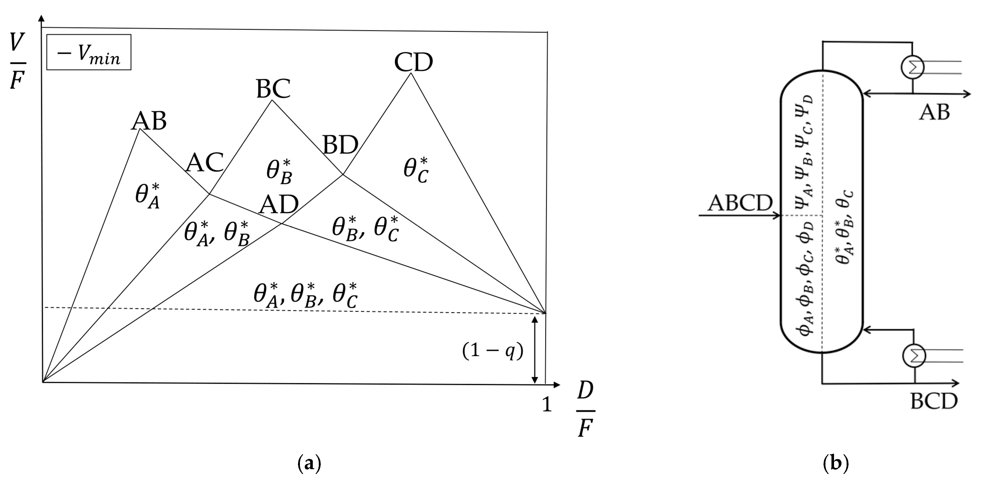
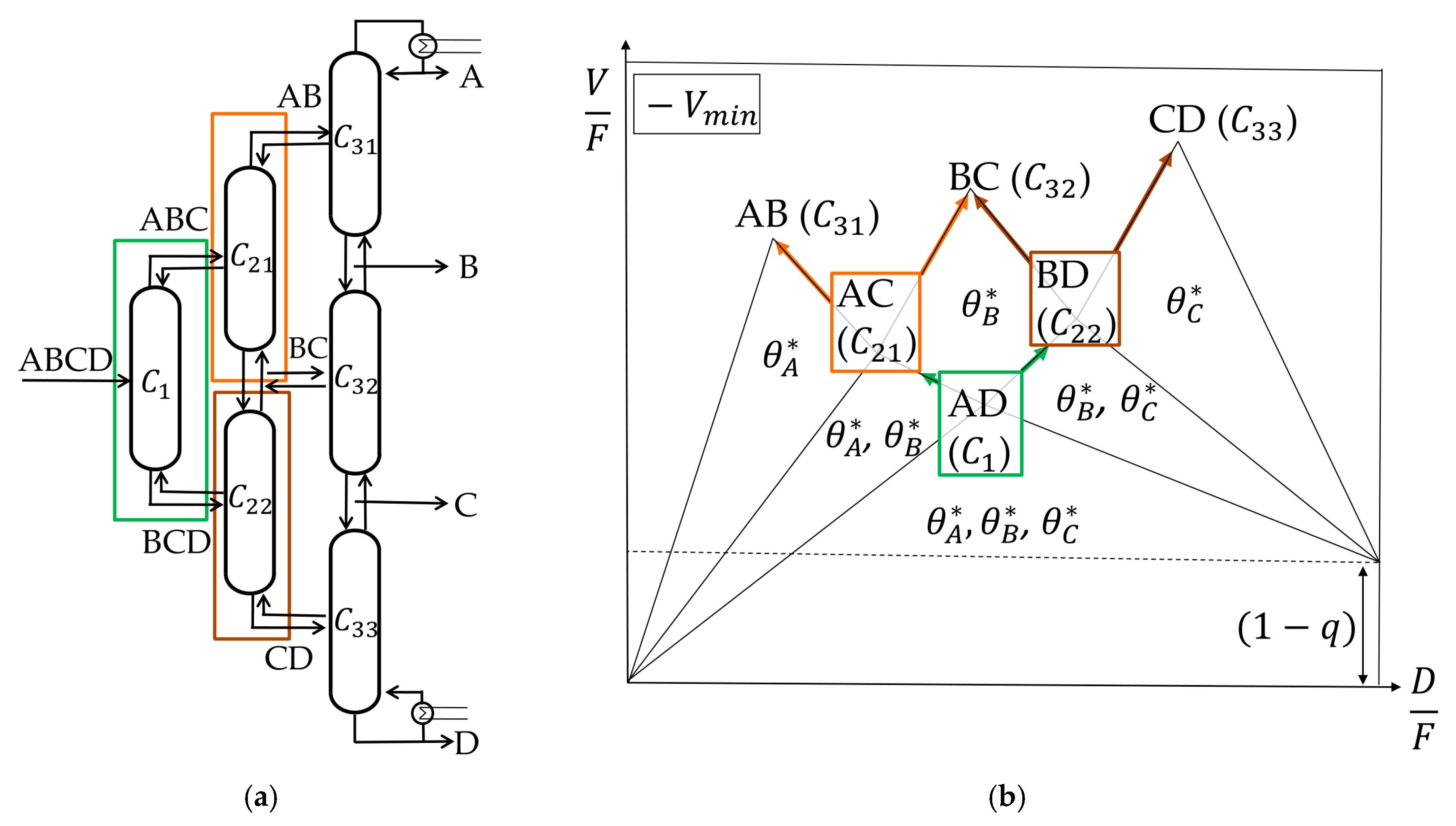
4.1. Petlyuk Cofiguration

In the Petlyuk configuration, each column splits the heaviest and lightest boiling components entering the column at the corresponding minimum vapor flow. This also means that the intermediate boiling components are distributed between the top and the bottom stream. It is said that the columns work at their preferred splits. For each column working at its preferred split, the actual Underwood Roots that carry over are also the common roots from the pre-sequent column. This means that the V_min diagram of a feed mixture in a conventional column is also valid for a Petlyuk configuration without changes. Note that the common roots θ_i can only carry over if they are active. Figure 5a shows a Petlyuk configuration and Figure 5b the corresponding V_min diagram.

The first column (prefractionator, C₁) splits component A and component D at the corresponding minimum vapor flow (its preferred split). This split is the lowest V_min point in the diagram. In this case, the common roots A, B, and C are active. In the column that is connected to the distillate stream of the prefractionator, C₂₁, component A is the lightest and C the heaviest boiling component which are split (again preferred split). The common roots A and B, lying between the volatilities of component A and C, carry over to this column. The same is true for the column connected to the bottom stream of the prefractionator (C₂₂). Component B is the lightest and D the heaviest boiling component. The roots B and C carry over and describe the split between the two components. The same is true for the following sharp splits without distributing components. As long as each thermally coupled column is allowed to work at its preferred split, the V_min diagram will not change. Note that the highest peak in the diagram shows the total necessary vapor needed to separate the feed mixture in a Petlyuk configuration.

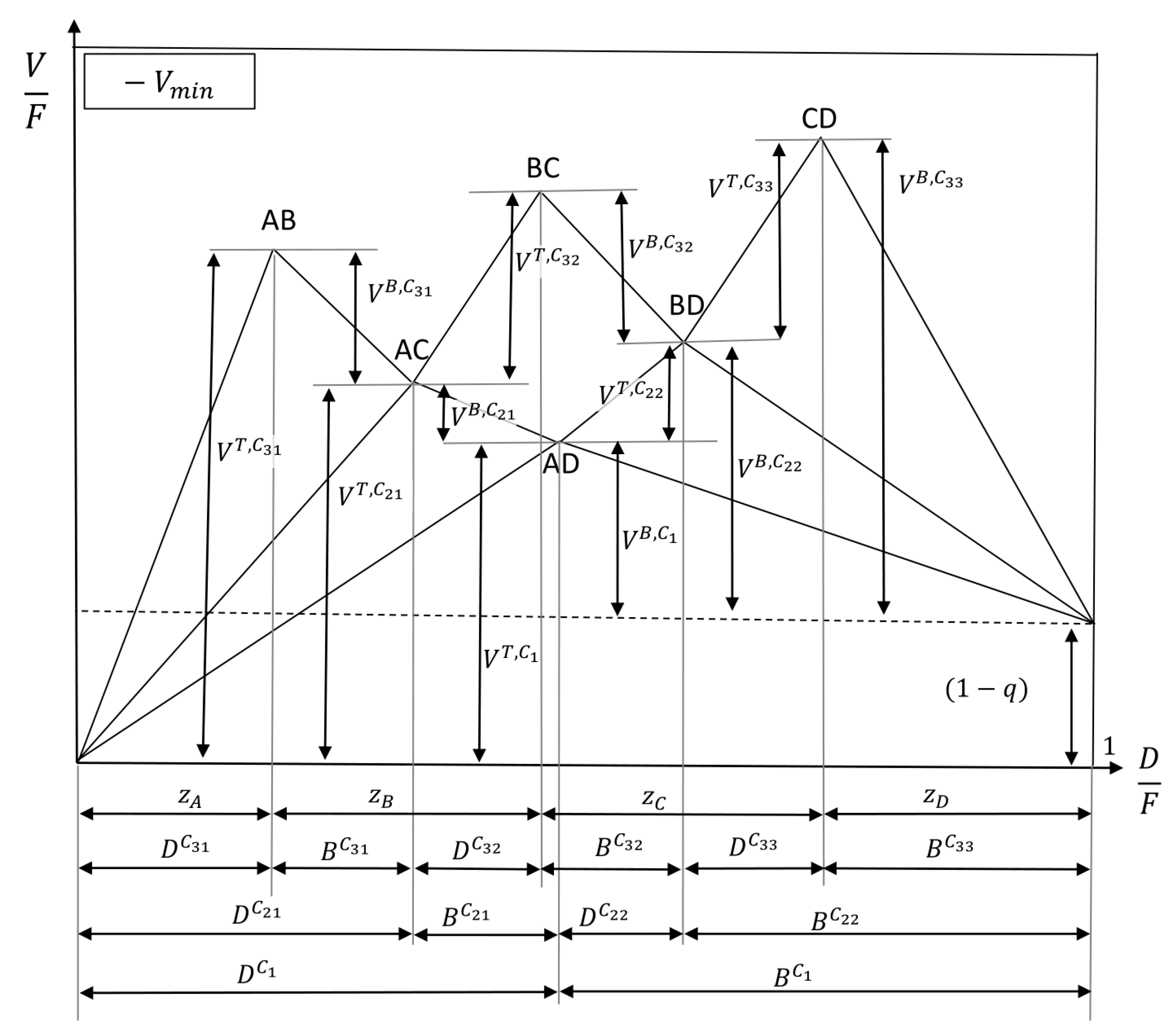
With the V_min diagram, all coupling streams in a Petlyuk configuration, meaning the vapor, as well as liquid streams, can be determined as shown in Figure 6.

The vapor streams can always be calculated by a balance around the particular columns. For example, the vapor stream at the top of column C₁ $\left(V^{T,C_1}\right)$ is the vapor stream entering at the bottom $\left(V^{B,C_1}\right)$ plus the amount of vapor in the feed stream (1 − q). The column C₂₁ is fed with the vapor of column C₁. Therefore, the internal vapor stream at the bottom of the column $\left(V^{B,C_{21}}\right)$ is the difference between the performed split (AC) and the prior split (AD) $\left(V^{B,C_{21}}=V_{min,AC}-V_{min,AD}\right)$. Internal liquid streams are determined by a molar balance at the head of the column, resulting in Equation (18).

$$L^{T,C_i}=V^{T,C_i}-D^{C_i}$$

(18)

Also note the difference between the vapor at the top and the bottom of the columns, for example, in column C₃₃, which performs the split between component C and D. The bottom stream is the vapor which is needed to separate C and D, including the prior split from A and B, which can also be written as the ABC|D split. The vapor in the top stream is only the vapor needed to split components C and D entering the column from the prior one. The internal feed stream entering only contains component C and D. This means that the top vapor stream only describes the vapor needed for the C|D split.

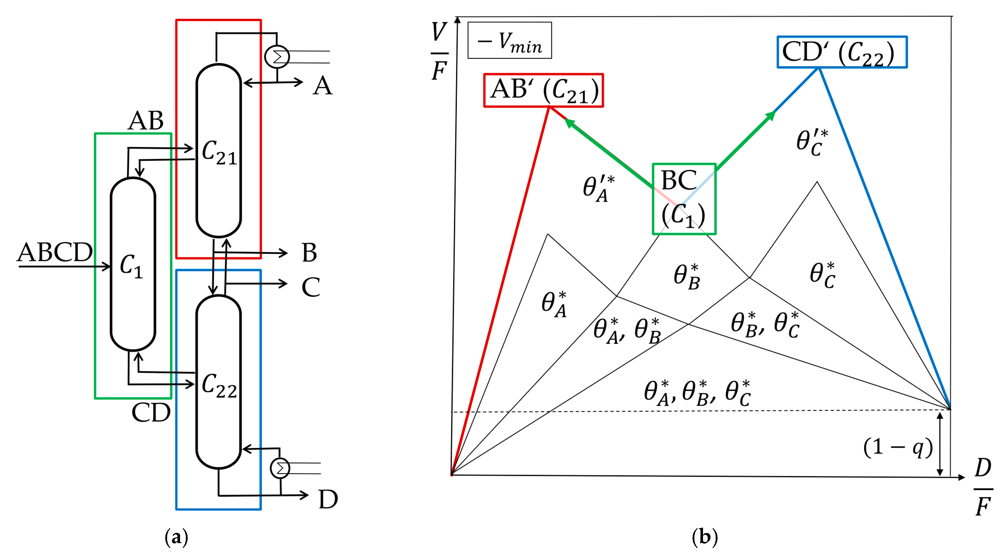
4.2. Kaibel Configuration

The Kaibel column is a simplified configuration that enables the separation of four components in one column shell with only one dividing wall. It is the only yet realized DWC to separate four component mixtures [7,17]. The corresponding thermodynamic equivalent sequence of thermally coupled columns is shown in Figure 7a. One major difference of the Kaibel column compared to the conventional Petlyuk sequence from Figure 5a is the split in the prefractionator. It is not working at its preferred split which is AD, but at a sharp BC split. Hence, the columns are no longer working in the most energy efficient way, resulting in a higher energy consumption of the Kaibel configuration compared to the Petlyuk configuration in any case [18]. The V_min diagram of the original feed is still valid, but only in the prefractionator, and at the BC instead of the AD split. The minimum vapor flow of the subsequent columns has to be recalculated and results in a change of the V_min diagram, as shown in Figure 7b. This is discussed in the following.

For feasible processes, the vapor flow in subsequent columns is always higher than in the pre-sequent. Accordingly, performing the column C₂₁ with a lower vapor stream than C₁ is impossible. Therefore, it is obvious that the V_min diagram must change. A closer look at the Underwood Roots also shows that the diagram has to be adapted. The only active root in C₁ is common root B θ_B because the BC split is performed, which is not the preferred one. The common roots A and C are not active and cannot carry over. Only the actual roots of the prefractionator carry over, which means that a performance at minimum vapor flow is no longer feasible. To determine the new V_min diagram for a Kaibel configuration, first the V_min diagram of the prefractionator C₁ is calculated, as described in Section 3.2.3. The active roots in C₂₁ θ_A’ and C₂₂ θ_C’ are calculated with a new feed equation, which is derived by a vapor balance around the corresponding column, as explained in Section 3.2.1. The resulting feed equation used to calculate θ_A’ in C₂₁ is shown in Equation (19).

$$V_{min,BC}=V^{T,C_{21}}-V^{B,C_{21}}={\displaystyle \sum }_{i=1}^n\frac{{\alpha }_i·z_i·F}{{\alpha }_i-{\theta }_A^{’}}·r_i^{T,C_1}=\frac{{\alpha }_A·F·z_A·r_A^{T,C_1}}{{\alpha }_A-{\theta }_A^{’}}+\frac{{\alpha }_B·F·z_B·r_B^{T,C_1}}{{\alpha }_B-{\theta }_A^{’}}$$

(19)

$V_{min,BC}$ is known from the V_min diagram which is valid in the prefractionator and the recoveries of A and B are one. The terms for component C and D were canceled out because their recoveries at column C₁ are zero. The resulting new minimum vapor flow for the AB split is shown in Equation (20). Due to the fact that vapor is fed to the middle of column C₂₁, the minimum vapor flow of the AB split equals the vapor flow at the top of the column (compare to Figure 6).

$$V_{min,AB}{}^{\text{'}}=V^{T,C_{21}}=\frac{{\alpha }_A·F·z_A}{{\alpha }_A-{\theta }_A^{\text{'}}}$$

(20)

The feed equation in column C₂₂ is also derived by a vapor balance. Now, component C and D are in the feed stream to column C₂₂ and $V_{min,BC}$ is a leaving stream instead of an entering stream. Equation (21) is used to calculate the new common root C (${\theta }_C^{\text{'}}$).

$$-V_{min,BC}+\left(1-q\right)·F=V^{T,C_{22}}-V^{B,C_{22}}={\displaystyle \sum }_{i=1}^n\frac{{\alpha }_i·z_i·F}{{\alpha }_i-{\theta }_C^{’}}·r_i^{B,C_1}=\frac{{\alpha }_C·F·z_C·\left(1-r_C^{T,C_1}\right)}{{\alpha }_C-{\theta }_C^{’}}+\frac{{\alpha }_D·F·z_D·\left(1-r_D^{T,C_1}\right)}{{\alpha }_D-{\theta }_C^{’}}$$

(21)

It is assumed that the composition of the vapor from C₂₂ to C₁ is the same as the one in the liquid stream leaving C₁ at the bottom to C₂₂. The recoveries of C and D in the top stream of C₁ are zero. Now note that the new common root ${\theta }_C^{\text{'}}$ is only valid for the feed stream entering C₂₂ only containing component C and D and not A and B. In addition to that, since there is vapor leaving the column at the middle, the minimum vapor for the CD split equals the bottoms vapor stream and not the top vapor stream. Based on this, Equation (22) is used for the calculation of the new CD split.

$$V_{min,CD}{}^{’}=V^{B,C_{22}}+\left(1-q\right)·F=V^{T,C_{22}}+V_{min,BC}-\left(1-q\right)·F+\left(1-q\right)·F=\frac{{\alpha }_C·F·z_C·r_C^{T,C_{22}}}{{\alpha }_C-{\theta }_C^{’}}+V_{min,BC}$$

(22)

with a recovery of component C at the top of column C₂₂ $r_C^{T,C_{22}}=1$.

Another possibility to determine the new common roots would be to calculate the actual roots in column C₁. Thus, also a vapor balance is made, but in this case, around C₁ instead of C₂₁/C₂₂, as shown in Equation (23) for the top section of C₁.

$$V^{T,C_1}=\frac{{\alpha }_A·F·z_A·r_A^{T,C_1}}{{\alpha }_A-{\Phi }^{C_1}}+\frac{{\alpha }_B·F·z_B·r_B^{T,C_1}}{{\alpha }_B-{\Phi }^{C_1}}=V_{min,BC}$$

(23)

with ${\Phi }^{C_1}={\theta }^{C_{21}}={\theta }_A^{\text{'}}$, both calculations result in the same values for the common roots in C₂₁ and C₂₂.

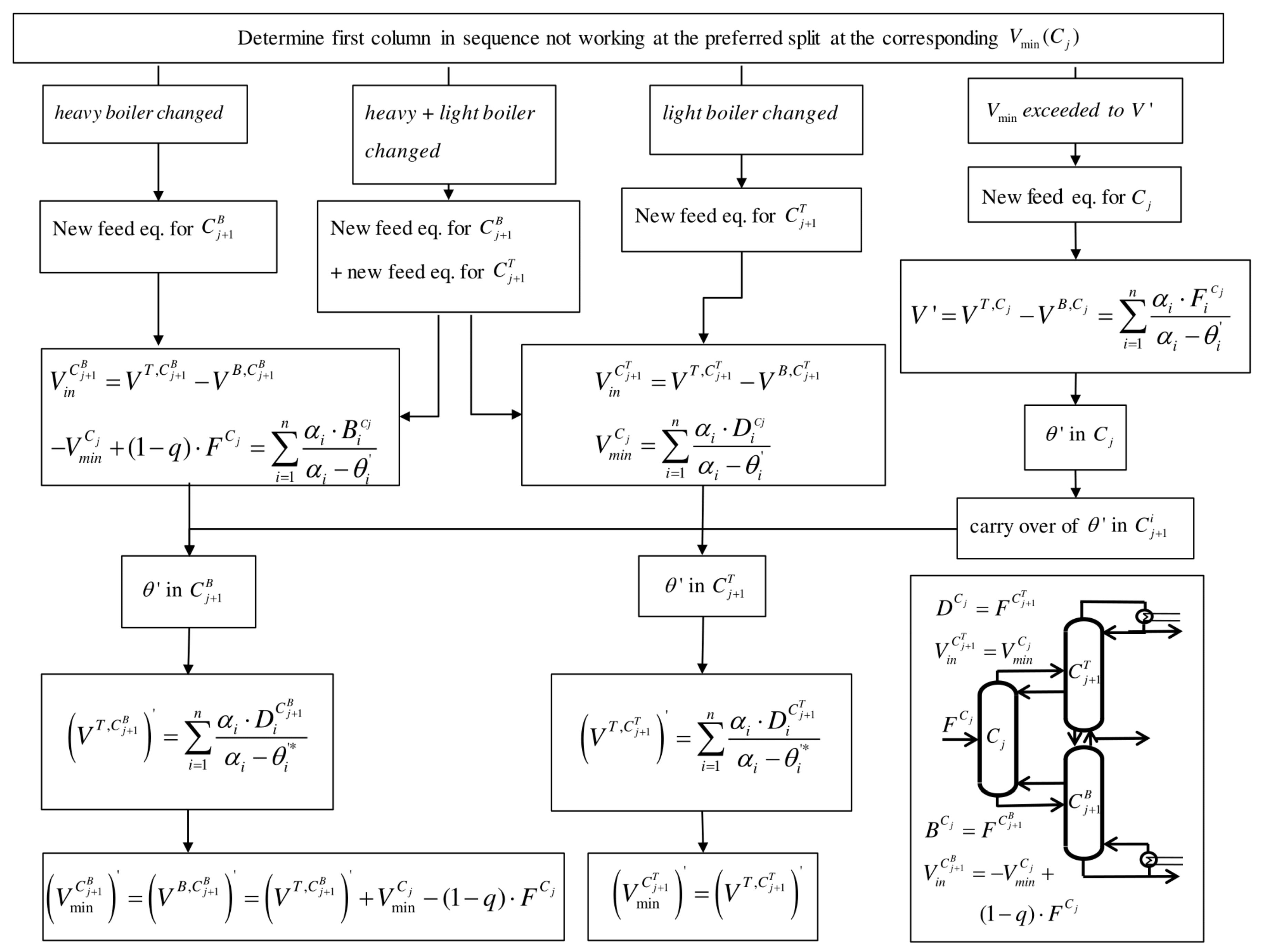
4.3. V_min Diagrams for Other Column Configurations

As explained before (Section 4.2), the V_min diagram changes as soon as one column does not work at its preferred split. This means that it does not perform the sharp split between the lightest and heaviest boiling component in its feed stream at the minimum vapor flow. This results in a change of the common and therefore active roots.

Adapted column configurations can be important in order to reduce the complexity of the process, for example, by minimizing the number of vapor splits, as presented by Ge et al. [13]. An adapted column sequence results in changes of thermal coupling and thus the V_min diagram. In order to obtain the new V_min diagram in the subsequent columns, a systematic procedure is suggested, as shown in Figure 8.

As soon as one column is not working at the preferred split, some of the common roots cannot carry over to the following columns. This can be the case if a split is skipped or if more vapor is provided than the minimum vapor necessary. Both cases result in a change of common root(s). In the first case, new common root(s) are calculated by determining the feed equation for the subsequent column. This is performed with a vapor balance as shown in Section 4.2. Note that the feed stream to the subsequent columns is different than the feed to the first column; for $C_{j+1}^T$, the feed is the distillate stream of $C_j$, and for $C_{j+1}^B$, it is the bottom stream of $C_j$. In the second case, more vapor is provided than necessary (V > V_min), which results in a new common root in the corresponding column which carries over to subsequent columns. Generally, the flowsheet in Figure 8 enables a total calculation of the V_min diagram based on the original feed composition, no matter which sequence of thermally coupled columns is used.

5. Initialization of Rigorous Simulation

For the initialization of a simulation via V_min diagrams, one point has to be considered if liquid side streams are assumed. No vapor leaving in side streams and assuming a feed with q = 1 means that the whole amount of vapor produced by the reboiler at the bottom of C₃₃ is leaving column C₃₁ at the top. This means that all sharp splits without distributing components are performed at the vapor amount of the most difficult split. Hence, for the case of liquid side streams, not the minimum vapor flow of each split can be implemented in the simulation [19]. There are also other methods to compensate for an excess of vapor, for example, a vapor side stream or a distribution of the vapor in the whole column arrangement instead of only in the columns in the last row. Small differences can be compensated for by using superheated or subcooled feed streams, as presented in [4]. Nevertheless, these cases will not be considered in this work.

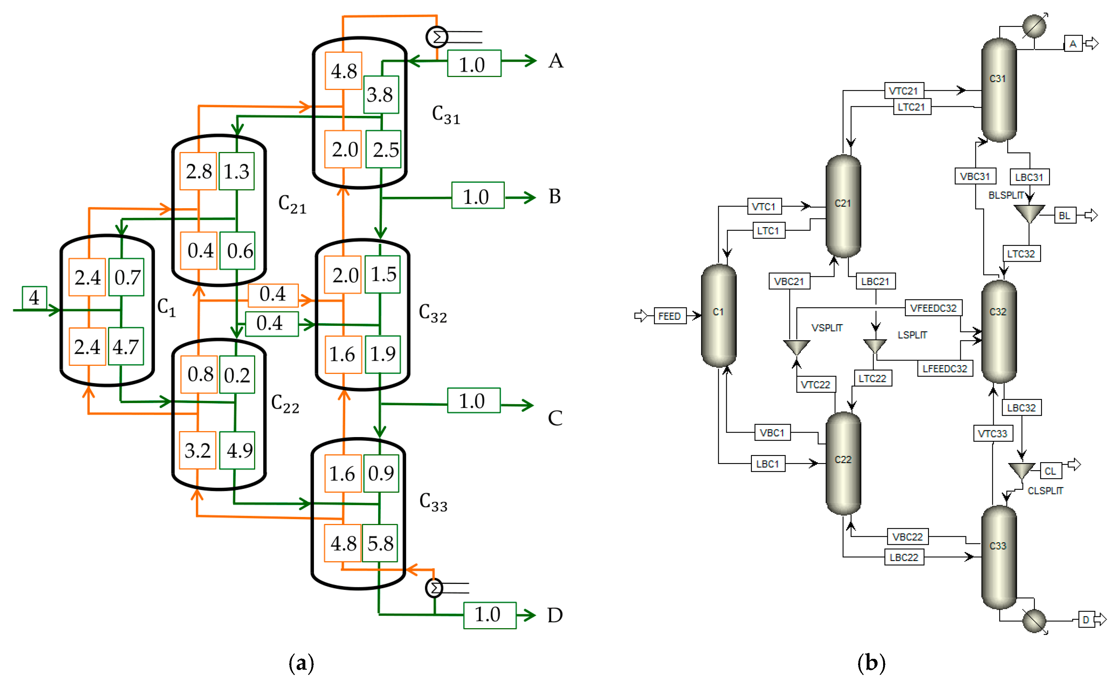
A multiple Dividing Wall Column model for the separation of four components is presented, which was simulated in Aspen Plus^®. It has to be kept in mind that an optimal solution is not searched for, and the main goal is to get a simulation that converges with the initial values. The system 3-Metylhexane (A)/Toluene (B)/Ethylbenzene (C)/1-Methyl-3-Ethylbenzene (D) was used for the simulation (z_i = 0.25). First, the V_min diagram was calculated, which is shown in Figure 9, with a MATLAB code performing the calculation presented in 3.2.3. K-values of the feed (q = 1) were determined in Aspen HYSIS^® and are all divided by the K-value of the heavy boiler 1-Methyl-3-Ethylbenzene according to Equation (2), resulting in α_i [7.5, 4.5, 2.2, 1].

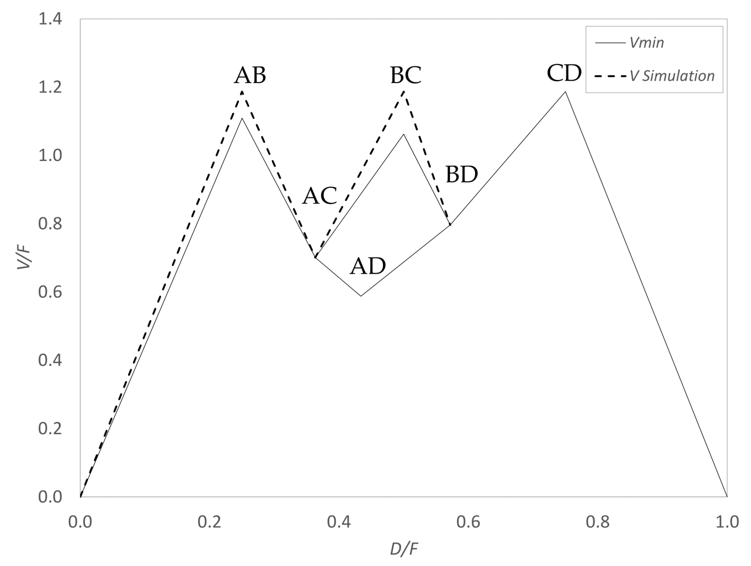
The most difficult split is the CD split. As explained before, this results in the same vapor amount at the AB as well as BC peak for the simulation, which is indicated as a dashed line in the diagram. Internal streams were read out according to Figure 6 and Equation (18), and a detailed description can be found in [12]. All internal streams determined with Figure 9 are shown in Figure 10a.

The simulation was performed as a six-column Petlyuk arrangement with liquid side streams implemented in Aspen Plus^®, as shown in Figure 10b. The column model RadFrac was used due to several reasons. First, columns without a condenser and reboiler are necessary. Second, some of the columns have to be fed with more than one feed stream. Third, the results are needed for each column stage. All three points are not available in the other models as DSTWU. For each column, 50 theoretical stages were assumed, which approximates an infinite number of stages. Feed streams from the pre-sequent columns always enter at the middle of the column at stage 25. To calculate thermodynamics, NRTL was used since all binary systems were fully defined.

Comparing the top streams of C₂₂ with the bottom streams of C₂₁ results in a liquid, as well as vapor stream, leaving the two columns to C₃₂. The streams in the opposite direction are neglected. Two splitters (LSPLIT and VSPLIT) were implemented to regulate the distribution of the streams. The values that were used for initialization are shown in

Table 3. Initial values used for rigorous simulation in Aspen Plus^®.

Variable	Unit	Value	zA (mol/mol)	zB (mol/mol)	zC (mol/mol)	zD (mol/mol)
VBC22	kmol/h	3.20	0.00	0.00	0.42	0.58
LTC21	kmol/h	1.40	0.69	0.31	0.00	0.00
LTC1	kmol/h	0.60	0.58	0.32	0.11	0.00
VBC1	kmol/h	2.40	0.00	0.20	0.36	0.44
A (distillate C31)	kmol/h	1
RB at C33	1	4.8
$BLSPLIT=\frac{BL}{LBC31}$	1	0.40
$CLSPLIT=\frac{CL}{LBC32}$	1	0.52
$LSPLIT=\frac{LFEEDC32}{LBC21}$	1	0.63
$VSPLIT=\frac{VFEEDC32}{VTC22}$	1	0.50

.

With the initial values shown in Table 3, a converging simulation was obtained. The purities of the components are shown in Equation (24).

$$\begin{gathered} x_A^A=99.9\% \\ {x}_B^{BL}=93.7\% \\ {x}_C^{CL}=93.3\% \\ {x}_D^D=98.9\% \end{gathered}$$

(24)

The mixture was separated successfully even though the product streams are not of high purity. This is caused by the three assumptions on which the Underwood method is based. These are constant molar flows, an infinite number of stages, and constant relative volatilities. The latter one was found to deviate up to 30% in terms of the values in the feed stream. Additionally, the molar flows were found not to be constant. Nevertheless, it is clear that with the short-cut initialization method of V_min diagrams simulation can be performed successfully.

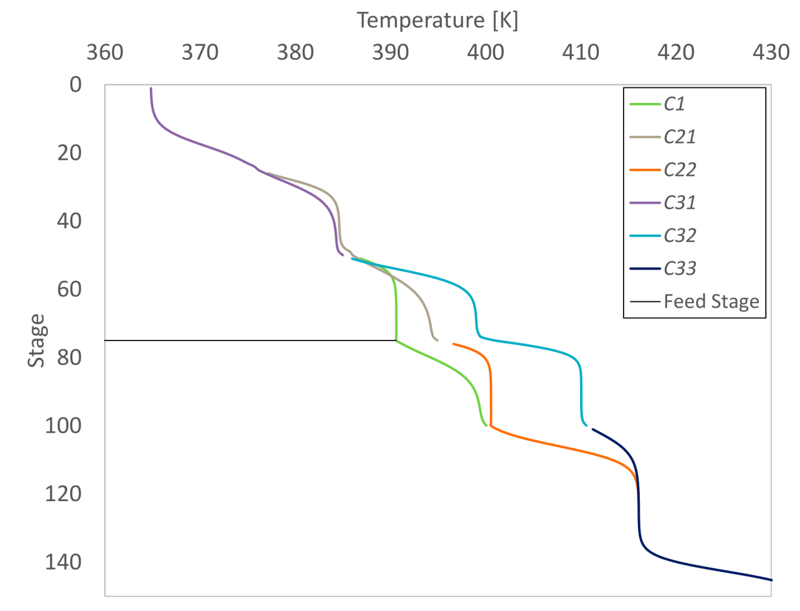
The temperature profile of the process is shown in Figure 11. Stage numbering starts at the top of the columns.

As typically seen for distillation columns, the temperature increases from the bottom to the top of the column. For the special case of Dividing Wall Columns, the temperature splits on different sides of the dividing walls. In the middle section around the feed stage, the temperature is the lowest in the prefractionating section (column C₁). The temperature has a higher value behind the first dividing wall (lower part of C₂₁ and upper part of C₂₂). A further increase can be noted in the last column row at the same stage as the feed (column C₃₂). At the liquid and vapor splits, the temperature profiles cross (for example C₂₁-C₁ at stage 50).

With this example, it was shown that the initialization of rigorous simulations with V_min diagrams is possible.

6. Summary

The main goal of this work was to present the V_min diagram as a robust tool to initialize rigorous simulations of mDWCs. First, the V_min method was presented, showing that the calculation procedure is always the same, independent of the number of components and the column configurations. First, the standard V_min diagram for one column is calculated. In order to do this, the first step is to determine the feed equation which is used to determine the common Underwood Roots of the original feed stream (Section 3.2.1). Second, the active roots are used to calculate the minimum vapor streams (Section 3.2.2). For every additional component, there is one equation and one unknown one, which raises the computational effort but does not change the general procedure. Afterwards, the equivalent column sequence describing the mDWC has to be evaluated. In any case, the V_min diagram calculated with the initial feed properties is at least valid in the prefractionator. If one of the columns does not work at its preferred split, the diagram changes for the subsequent columns. New roots are calculated by determining a new feed equation around the respective column (Section 4.3), which are again used to calculate the minimum vapor amount (Section 3.2.2). In the end, it could be proven that initialization of rigorous simulations with V_min diagrams in a robust and fast way is possible (Section 5).

In summary, the V_min diagram is a simple short-cut method that can effectively be used to initialize rigorous simulations, which in the end, can be used to construct complex multiple Dividing Wall Columns.