Optimizing the Use of Chemical Inhibitors in Oil and Gas Fields by Developing Cost-Effective Strategies

Abstract

Corrosion, salt deposition, and biofouling critically impair flow assurance and mechanical integrity in oil and gas production systems, resulting in escalating operating costs and environmental burdens. This study presents a screening-level multi-criteria decision-making framework grounded in petroleum engineering practice. Unlike conventional MCDA approaches that require extensive laboratory testing for each asset, our model enables the rapid assessment of inhibitor transferability between technologically similar fields using normalized field parameters and actual procurement data. The model integrates a correlation analysis of the key field parameters of temperature, acid gas content, salt concentration, flow velocity, and water cut with a weighted effectiveness coefficient. A dataset of operational records was coupled with factual procurement prices from 2020 to 2025 to simultaneously optimize inhibitor type and dosing. The novelty lies in the multiplicative weighting scheme and the concept of critical deviation thresholds, which allow engineers to identify cost-saving opportunities without compromising the 90% protection target. Application of the model presented in this article allows a reduction in annual chemical-related operational expenditures. The proposed methodology provides petroleum engineers with a robust, data-driven screening tool to design cost-effective chemical treatment strategies that maintain corrosion protection and reduce environmental load, thereby advancing oil field chemistry technology and supporting efficient oil and gas field development.

1. Introduction

The contemporary oil and gas sector faces a complex interplay of technological, economic, and regulatory challenges that underscore the importance of research into the use of chemical reagents [1,2,3]. On one hand, corrosion inhibitors, scale-preventing agents, biocides and anti-paraffin/bitumen deposition chemicals are an objective technological necessity. These formulations ensure fault-free production processes, stable output and reliable transportation of hydrocarbon feedstock, preventing premature equipment failure [4,5]. On the other hand, the scope of chemical usage constitutes a substantial share of both operating (OPEX) and capital (CAPEX) costs for companies, thereby highlighting the importance of economic optimization to a priority scientific-practical task [6,7]. The core economic dilemma lies in the conflict between the technological imperative to apply reagents comprehensively and the exponential growth of associated expenditures that directly inflate the cost of final products [8]. This problem is compounded by an interrelated set of factors: market risks—difficulties in replacing highly specialized reagents, coupled with a trend toward monopolization of specific segments of the oil field chemicals market—generate critical price pressure and threaten shortages of essential formulations [9]; cost inefficiency arises when sub-optimal products are used, leading to direct financial losses including purchase and logistics costs as well as hidden expenses for mitigating the consequences of inadequate performance, such as unscheduled repairs of corroded equipment, cleaning from deposits, and forced downtime of facilities [3]; and high implementation cost and extensive duration of laboratory and pilot-plant testing of new reagents require significant time and financial resources, delaying the realization of a positive economic effect.

The environmental dimension deserves special attention. The use of chemical reagents in oil extraction and processing inevitably increases anthropogenic pressure on the environment. Risks of toxic compounds entering the atmosphere, water bodies and soils during normal operations and especially during accidental spills pose a direct threat to ecological safety [4,5]. This necessitates not only improved monitoring and protection systems but also a reassessment of reagent selection that incorporates ecotoxicological characteristics and potential ecosystem damage. Therefore, economic evaluation of chemical use must include not only direct costs but also environmental expenses associated with minimizing negative impacts and eliminating pollution consequences [6].

Despite these challenges, the sector retains significant cross-functional optimization potential. A promising direction is the adaptation of successful reagent applications across subsidiaries operating under similar geological–technical conditions. However, transplanting technology without scientific justification carries risks of misfit to a particular site’s specifics and requires a validated methodology that minimizes such risks and avoids unwarranted expenditures.

It is important to clarify the scope and novelty of the proposed approach. The methodology does not aim to replace laboratory and pilot plant testing of new inhibitor formulations; such testing remains a mandatory prerequisite for introducing any chemical reagent into field operations, as it validates both the corrosion inhibition efficiency and the compatibility with specific process fluids. Instead, the present work addresses the subsequent stage: once a reagent has been successfully tested and incorporated into the corporate inventory of approved chemicals, the question arises whether this same reagent can be economically transferred to another asset with comparable technological conditions, thereby avoiding repeated and costly qualification trials.

In this context, the novelty of our contribution lies in the development of a multiplicative screening model that formalizes the similarity assessment between assets. Unlike conventional MCDA frameworks that typically rely on static expert weights and linear additive aggregation, our model employs the following:

• A normalized dimensionless effectiveness coefficient for each technological parameter.
• Parameter-specific weights derived from a structured literature- and expert-based procedure.
• The concept of critical deviation thresholds that quantify the maximum permissible drift from the reference operating point while maintaining the target protection level (E_target = 90%). This enables a rapid, data driven compatibility check, reducing the need for repeated experimental campaigns.

Compared to traditional TEA (techno-economic analysis) and LCCA (life-cycle cost assessment), which typically evaluate a single asset over its entire life-cycle, our model focuses on the operational reallocation of existing reagents among multiple assets, capturing immediate OPEX reduction opportunities through the use of actual procurement prices from 2020 to 2025. The economic evaluation is thus anchored in current market realities rather than generic cost assumptions.

The aim of this study is to develop a screening-level methodology for the economic justification of chemical reagent selection and application in the oil and gas sector. Specifically, we construct an economic–mathematical model whose objectives are as follows:

• Conduct an analytical review of contemporary approaches to economically justifying the use of chemical reagents on oil field enterprises and identify their limitations.
• Analyze and systematize existing practices for selecting and applying major classes of chemical reagents–corrosion inhibitors, scale-preventing agents, biocides and others—using several subsidiaries of an oil–gas holding as examples.
• Perform a correlation analysis of key technological parameters involved in reagent application (dosage, environmental conditions, and effectiveness) and associated economic indicators (reagent cost and costs due to failures).
• Based on the analysis, develop a methodology for economically justifying the choice of chemical reagents that includes a decision-making algorithm and a system of differentiated criteria—technological and economic—with assigned weights.
• Build an economical—mathematical model formalizing the proposed methodology, enabling simulation modeling to evaluate cumulative costs and economic effectiveness across various reagent application scenarios.
• Validate the developed methodology and model on generalized data gathered during the analytical review and calculate the expected economic effect of their implementation.
• Formulate practical recommendations for implementing the research results to establish a corporate decision-support system in the field of oil–gas chemistry.

The novelty of the present study can be summarized as follows:

• Introduced a multiplicative screening model that links normalized technological parameters with actual procurement prices to assess the feasibility of inhibitor transfer between assets.
• Formalized the concept of critical deviation for each parameter, providing engineers with a practical tolerance interval that preserves 90% of protection effectiveness.
• The weight coefficients, derived from a structured literature- and expert-based procedure, were designed for iterative calibration as operational data accumulate, making the model adaptable to specific field conditions.

The economic evaluation is grounded in real market data (2020–2025), ensuring practical relevance for corporate procurement and inventory management.

2. Methods

As the methodological basis for optimizing operating costs of oil field chemical usage, an adaptive transfer approach was chosen that assumes the use of successful technological solutions in adjacent or analogous conditions. However, the specificity of the production environment imposes strict constraints: any economic optimization cannot be carried out at the expense of technological effectiveness and process safety. Consequently, the search for cost-reduction opportunities must proceed strictly within the bounds of a technological range of alternatives defined by permissible equipment operating regimes and reagent characteristics.

The key difficulty in formalizing such a problem lies in the heterogeneity of the raw data. Technological parameters that influence inhibitor protection efficacy have different physical natures and incompatible units of measurement (flow rate, temperature, chloride content, pressure, etc.). To bring them into a unified, dimensionless form and to correctly assess each factor’s contribution to the resulting indicator, an apparatus of normalized coefficients was applied. This approach allows a specific parameter to transform from absolute parameter values to their relative deviations from reference (optimal) values.

The basic assumption of the model is that the loss of inhibitor protection effectiveness is directly proportional to the absolute deviation of a current parameter value $x_i$ from its optimal (target) value $x_{opt,i}$. It is, however, obvious that different factors influence the final result unequally: changes in some parameters can critically affect the protective properties of the reagent, whereas fluctuations in others may be negligible. To quantitatively account for this sensitivity, each parameter is assigned a weighting coefficient ${\omega }_i$ that takes values in the interval $0<{\omega }_i\le 1$. The higher the weight, the more critical the deviation of that factor from optimum is with respect to the loss of protective effects.

Based on physical meaning and model requirements, the sought efficiency coefficient $E_i$ (characterizing a single parameter’s contribution to overall effectiveness) must satisfy the following boundary conditions:

• E_i = 1 when x_i = x_opt,i, corresponding to no deviation and thus an ideal parameter value;
• The function E_i monotonically decreases with the absolute deviation |x_i − x_opt,i|;
• The rate of decrease (steepness of efficiency drop) under equal conditions is higher when the weighting coefficient ω_i is larger, i.e., when the parameter is more significant for the inhibition process.

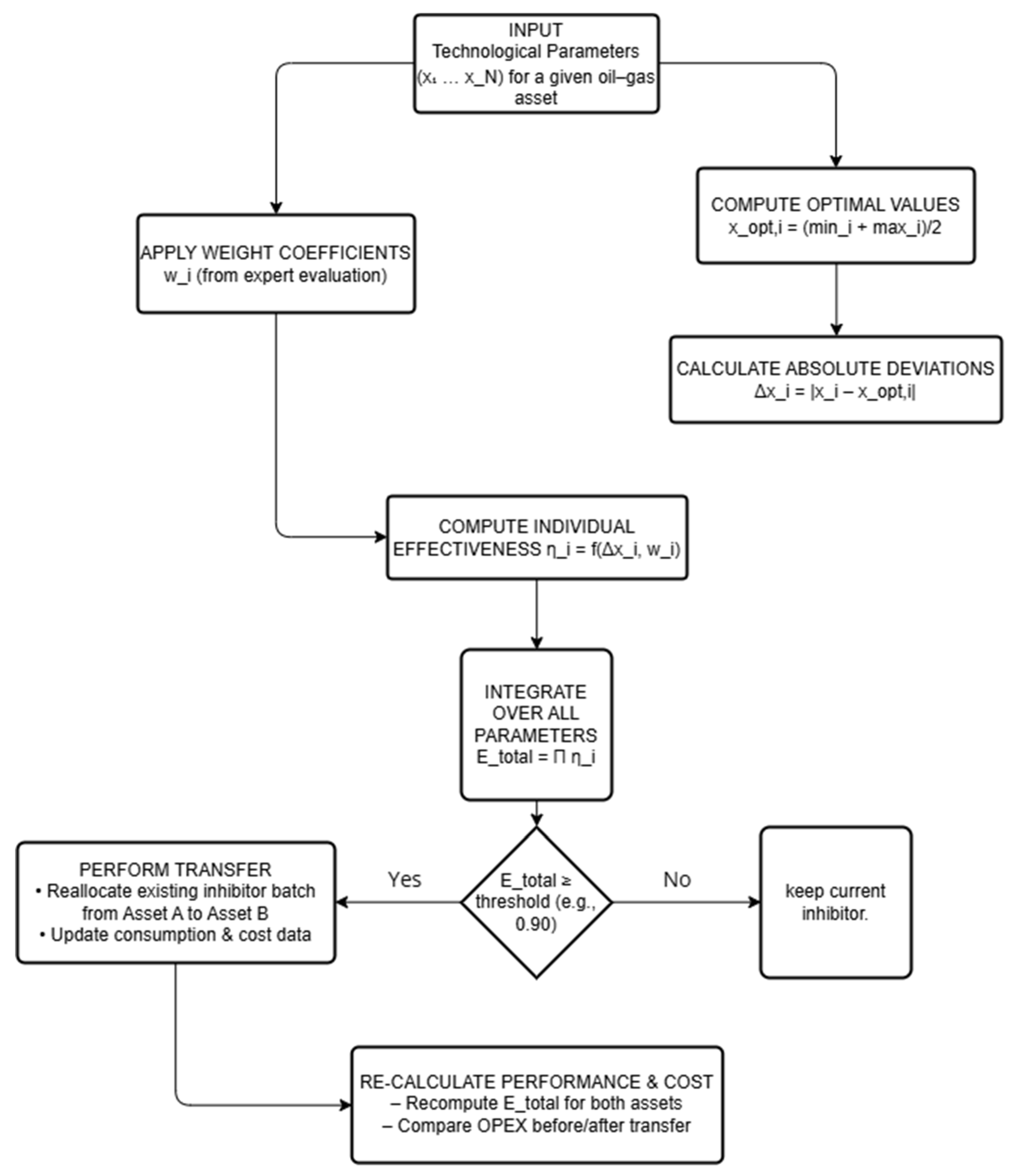
The logic derived from these boundary conditions and weighting principles can be operationalized into a stepwise decision-making workflow. This procedure, summarized schematically in Figure 1, translates heterogeneous field data into a dimensionless composite efficiency index, which then serves as the gating criterion for inhibitor application logic.

In the decision-making workflow (Figure 1), the term “reallocate the inhibitor from Asset A to Asset B” denotes a logistical substitution: the asset under consideration switches from its originally assigned reagent to a different product already present in the corporate inventory, provided that the effectiveness screening confirms its suitability. This may involve either a change in procurement specification (brand replacement) or, where physically feasible and cost-effective, the transfer of existing stock. The model itself does not mandate physical movement of chemicals; it identifies optimal combinations of “asset—inhibitor brand” based on technological similarity and procurement costs.

2.1. Initial Data and Scope of Application—Operational Dataset

2.1.1. Representative Parameter Ranges for an Oil-and-Gas Condensate Field

In the next table we present compilation of representative parameter ranges for an oil-and-gas condensate field (

Table 1. Parameter Ranges and Their Role as a Reference Basis.

Parameters	Minimum	Maximum	Average	Unit
Temperature	40.00	80.00	60.00	°C
H2S concentration	0.50	4.00	2.25	% vol.
CO2 concentration	0.30	1.50	0.90	${10}^3$, ppm
O2 concentration	0.05	5.00	2.525	${10}^{-3}$, % vol.
Chloride content	50.00	250.00	150.00	$\mathrm{g}{\mathrm{L}}^{-1}$
pH of aqueous phase	5.50	7.00	6.25	–
Flow velocity	1.00	5.00	3.00	$\mathrm{m}{\mathrm{s}}^{-1}$
Inhibitor concentration	50.00	150.00	100.00	ppm

) [7].

The mean values of each parameter range were selected as the reference point for normalization, rather than as a true technological optimum. This choice reflects standard industrial practice: an oil and gas enterprise, when introducing chemical reagents under a given set of technological parameters, first identifies the reagent that demonstrates the highest performance under those nominal conditions, and only then deploys it within the facility’s regular chemical line-up. Thus, the midpoint of the parameter interval corresponds to the conditions for which the most effective reagent has already been established, allowing the mean to serve as a legitimate reference for comparative assessment. Importantly, if the model is applied to assets with different operating envelopes, the reference point can be intentionally shifted toward the lower or upper boundary, for example, towards lower H₂S concentrations or lower temperatures, where inhibitor performance is typically more favorable. Such displacement allows the user to delineate the subset of assets for which adaptive transfer remains viable under deliberately tightened or relaxed limits.

Furthermore, this optimum can, when necessary, be intentionally shifted toward either the upper or the lower boundary of the parameter range. Such a displacement makes it possible to delineate the subset of assets for which adaptive transfer remains viable under deliberately relaxed or tightened operational limits, i.e., to determine the precise object pool that can accommodate re-allocation of the inhibitor without compromising the required technological effectiveness.

2.1.2. Distribution and Justification of Weight Coefficients

To assemble a dataset adequate for statistical analysis and model construction, we collected 5000 real operational combinations of the specified parameters from two years of field measurements at multiple sites within the oil-and-gas complex. The recorded values span the full defined ranges, reflecting the natural variability inherent in production conditions.

This empirically derived dataset forms the foundational input for the parametric analysis that underpins the development of our economical–mathematical model.

The pivotal stage in constructing the model is determining the contribution (weight) of each technological parameter to the integrated inhibitor-effectiveness indicator. Because a direct quantitative assessment based solely on raw field measurements is often impractical, we adopted an expert-evaluation approach grounded in a systematic analysis of fundamental physical–chemical mechanisms and corroborated by industry-wide literature and historical operational data.

For the systematic database and qualitative assessments, source [7,8] was used, supplemented with sector reports and standard corrosion models (Butler–Volmer equation, corrosion-rate correlations). Determining a quantitative measure of influence (weight coefficient) for each technological and reagent parameter on the overall inhibitor effectiveness is a core task in model construction. In the absence of a historical operational dataset for a specific field, a structured expert-evaluation approach based on critical analysis and synthesis of complementary sources was applied. This approach transforms qualitative descriptions and empirical dependencies known from the literature and practice into a formalized system of quantitative ratings [9,10].

The methodology comprises three interrelated components:

• Basic expert framework—the authoritative reference “Engineer’s Guide to Oilfield Chemicals and Fluids” (Infinity Energy Solutions) served as the primary source of systematic knowledge. It offers a ranked description of key factors (e.g., H₂S concentration, inhibitor dosage, water-phase mineralization) affecting chemical protection efficacy, providing a starting point for assigning high-order base weights (0.6–0.7) [11].
• Contextual adaptation and physical-chemical justification—to tailor the general principles to conditions relevant to an oil-and-gas condensate field, the base estimates were critically adjusted based on the following:

  ○

  Industry data—analysis of sector reports (including those from major production operations) allowed the incorporation of specific fluid compositions and typical operating ranges (e.g., a relatively low standard oxygen content led to a weight of 0.1 for O₂).

  ○

  Fundamental models—for parameters with clear theoretical dependencies, weights were justified through these models (e.g., the flow-velocity weight of 0.4 is derived from a quadratic relationship between erosion wear and Reynolds number thresholds that trigger turbulence and film failure).

  ○

  Empirical correlations—published experimental and field data verified the weights (e.g., a weight of 0.6 for mineralization is supported by a linear correlation, documented in studies conducted at leading corrosion research laboratories, between chloride concentration and the pitting corrosion rate, directly reducing inhibitor effectiveness) [12,13].

• Internal consistency principle—the final weight system was checked for logical consistency. Parameters sharing a common physical mechanism (e.g., H₂S and pH affecting proton activity) were cross-validated to avoid over-estimation of interdependent factors, ensuring model balance [14,15].

The outcome of this methodology is the set of weight coefficients shown in

Table 2. Weight coefficients for parameters influencing inhibitor effectiveness.

Parameters	Rationale & Brief Explanation (Based on Source Analysis)	Weight (${\mathit{\omega }}_{\mathit{i}}$)
Temperature	B Thermal desorption of inhibitor reduces efficacy by 30–50% in 40–80 °C range	0.50
H2S concentration	Directly competes with inhibitor for active sites, near-zero effectiveness without dedicated inhibition	0.70
CO2 concentration	Enhances acidification, increasing corrosion rate	0.40
O2 concentration	Minor effect in closed systems but can contribute to cathodic reactions	0.10
Chloride content	High chloride destabilizes protective film, accelerates pitting	0.60
pH of aqueous phase	Stability window of many amine-based inhibitors	0.20
Flow velocity	Erosion–corrosion scales with v2, turbulence accelerates film removal	0.40
Inhibitor concentration	Threshold behavior of adsorption layer formation, critical for continuous protection	0.70

. Each value was preceded by an analysis that considered both its absolute impact on corrosion processes and its relative importance within the specific technological context of the modeled field.

It should be emphasized that the proposed model operates within the constraints of an existing corporate reagent portfolio, where each candidate inhibitor has already undergone mandatory laboratory and field pilot qualification in accordance with industry standards (e.g., NACE SP0108 or analogous corporate protocols) [16]. Consequently, the primary chemical and compatibility risks—such as emulsion formation, scaling tendency, or incompatibility with produced water—have been screened out prior to inclusion in the portfolio [12,17]. The model’s role is not to replace such testing but to identify, among the already qualified reagents, the most cost-effective option for a given set of operating conditions, based on the similarity of key technological parameters. The physical–chemical rationale behind each weight coefficient (Table 2) is grounded in well-established mechanisms: for instance, the high weight assigned to H₂S concentration reflects its direct competition with inhibitor molecules for active adsorption sites on the metal surface; the weight for temperature accounts for thermally activated desorption [12]; and the weight for chloride content is justified by its well-documented role in pitting corrosion acceleration [18,19].

The sum of the weight coefficients is deliberately not normalized to unity. This design choice is mathematically advantageous for the multiplicative structure of the model (Equation (2)), where weights are used as exponents of the deviation ratio. In this formulation, weights represent the sensitivity multipliers of each parameter’s influence on the overall effectiveness, rather than probability-like importance scores. Normalizing to unity would impose an arbitrary constraint—a reduction in one weight would force an increase in another—which does not reflect the independent physical nature of the parameters [12]. For instance, the influence of H₂S concentration on inhibitor adsorption is not mechanically linked to the influence of flow velocity; each factor acts through distinct physical mechanisms [12,17]. The unnormalized weight system preserves this independence and allows each weight to be calibrated individually as empirical data accumulate, without affecting the relative importance of other parameters.

It is important to note that the sum of the weight coefficients is deliberately not normalized to one. In the proposed economical–mathematical model they are used as multipliers of relative significance when computing a weighted integrated effectiveness indicator ($E_i$), rather than as probabilities. This approach visually ranks factors by the strength of their influence and accurately incorporates their contribution in a multi-factor model where the final effect arises from parameter interaction, not simple additive accumulation.

2.2. Coefficient of Effectiveness for an Individual Parameter

To assess the contribution of each individual parameter within a given technological combination, a normalized effectiveness coefficient $E_i$ was calculated using Formula (1):

$$E_i=1-{\omega }_i·{\displaystyle \frac{\left|x_i-x_{opt,i}\right|}{x_{max,i}-x_{min,i}}}$$

(1)

where $E_i$ is the effectiveness coefficient for the $i$ parameter, indicating how close the current value is to optimum, ${\omega }_i$ is the weight coefficient reflecting the influence of the $i$ parameter, $x_i$ is the current value of the parameter in the combination, $x_{opt,i}$ is the optimal (target) value, taken as the arithmetic mean of the range boundaries, $x_{max,i}$ is the maximum value of the parameter, and $x_{min,i}$ is the minimum value of the parameter.

This formula guarantees that $E_i=1$ when $x_i=x_{opt,i}$ and that $E_i$ decreases monotonically as the parameter deviates from its optimum, proportionally to its weight ${\omega }_i$.

2.3. Integrated Indicator of Overall Effectiveness

The overall effectiveness of inhibitor application for each set of parameters ($E_{total}$) was defined as the product of the individual effectiveness coefficients across all considered parameters in Formula (2). This multiplicative approach captures the compounded impact of all factors, whereby deterioration in any single factor reduces the total outcome.

$$E_{total}=\prod _{i=1}^n{E}_i$$

(2)

where $n$ is the number of controlled parameters.

The integral indicator $E_{total}$ thus obtained quantitatively characterizes the overall inhibition effectiveness for a given set of technological parameters and serves as an objective criterion in the adaptive transfer procedure. This is according to the decision-making logic (Figure 1).

2.4. Determination of Critical Parameter Deviations

For practical application of the model, it is useful to define the boundary conditions under which the system retains acceptable performance. We introduce the concept of a critical parameter deviation as the maximum absolute deviation $∆x_i^{critical}$ from the optimal value $x_{opt,i}$ at which the overall effectiveness $E_{total}$ does not fall below a prescribed threshold $E_{threshold}$, assuming all other parameters are fixed at their optimal levels.

With the remaining parameters fixed, $E_{total}=E_i$, and setting $E_{threshold}=90\mathrm{\%}$, the condition becomes $E_i=1-{\omega }_i·{\displaystyle \frac{\left|x_i-x_{opt,i}\right|}{x_{max,i}-x_{min,i}}}\ge E_{threshold}$, and solving for the inequality yields the formula for calculating the critical deviation:

$$∆x_i^{critical}={\displaystyle \frac{1-E_{threshold}}{{\omega }_i}}·(x_{max,i}-x_{min,i})={\displaystyle \frac{0.1}{{\omega }_i}}·(x_{max,i}-x_{min,i})$$

(3)

This expression provides a quantitative criterion for assessing whether a given technological parameter remains within the safe operating window. The calculated critical deviations for each parameter are presented and analyzed in Section 3 (Results), where their practical implications for inhibitor selection are discussed.

2.5. Development and Formalization of the Model

The model was developed in a sequential manner: during the formalization stage, a representative set of input data is analyzed and an integrated technological indicator is defined, providing the foundation for the subsequent economic assessment of the adaptive reagent-transfer methodology. The key link that connects the technical calculations to the economic analysis is the financial-parameter block, which incorporates the capital cost, unit cost of the reagent and its technological dosage. These parameters are calculated using up-to-date external data and industry norms, thereby enabling a transition from technological effectiveness to a comprehensive economic evaluation.

2.5.1. Determination of the Discount Rate

The average key rate for each year was calculated as a weighted mean, where the weights correspond to the number of days each rate value was in effect during that calendar year. Formally, for each year $Y$ the average rate ${\overline{R}}_i$ was computed using Formula (4):

$${\overline{R}}_i={\displaystyle \frac{{\sum }_{\mathrm{d}=1}^m(R_d·D_d)}{D_Y}}$$

(4)

where $R_d$ is the key rate value in annual percentage terms, $D_d$ is the number of days during which $R_d$ was active within year $Y$, $D_y$ is the total number of days in year $Y$, and $m$ is the number of distinct rate values observed in year $Y$.

Applying this methodology to the 2020–2025 data yielded the yearly average key rates presented in

Table 3. Results of calculating the annual average key rate.

Year	Average Key Rate, % per Annum
2020	5.02
2021	5.94
2022	10.17
2023	10.44
2024	15.93

. These values are used as the risk-free discount rate in the subsequent economic calculations.

These data serve as the basis for calculating the present value in subsequent economic modeling.

2.5.2. Calculation of the Unit Cost of the Inhibitor

Determining the unit cost of an inhibitor (price per ton of reagent) is a critically important step for building the economic component of the model. In a highly volatile chemical reagent market, the use of actual, up-to-date market data ensures the adequacy of subsequent economic effectiveness calculations. To achieve maximum relevance and objectivity, the base price is not derived from aggregated market reviews but instead extracted directly from real purchase data of large oil-and-gas companies. The inhibitor manufacturers considered in this paper are LLC “Mirrico”, LLC “NPC “InTechProdService”, JSC “PolyEx”, JSC “SNPKH”, JSC “NPC “ChemTechno”, and JSC “OZNH”, with the official procurement portal serving as the primary information source.

For this calculation, several competitive procurement procedures for corrosion inhibitors conducted between 2020 and 2025 were analyzed. For each procedure, the unit cost was obtained by dividing the total contract value by the delivery volume.

To bring all cost figures to a common reference point, every obtained unit cost was then adjusted to the planning horizon—the end of 2025. This adjustment was made by discounting each original cost using the annual key rate of the central bank as the risk-free rate: the original unit cost for a given procurement year was compounded forward over the number of years separating that year from 2025.

The results of the calculation are summarized in

Table 4. Calculated historical unit cost of the inhibitor.

Reagent Number	Year	Original Unit Cost, usd./t	Present-Value Unit Cost, usd./t
1	2024	1929	2237
2	2025	2314	2314
3	2020	1645	2582
4	2024	2338	2710
5	2024	2328	2699
6	2024	2329	2701
7	2024	2364	2741
8	2024	2035	2359
9	2024	2155	2498

.

2.5.3. Normalization of Reagent Consumption

Determining a rational inhibitor dosage for each specific operating scenario is a pivotal problem that sits at the intersection of physical–chemical kinetics and industrial economics. The proposed method rests on the principle of reasonable sufficiency: finding the minimum reagent concentration that guarantees attainment of the required protection level (target effectiveness $E_{threshold}$).

The intensity of inhibitor injection (consumption per unit time) directly depends on two key parameters: the volume of fluid being pumped and the requisite chemical concentration [15]. For a straight pipe section of a constant cross-section, the volumetric flow rate of inhibitor $Q_{inhibitor}$ is defined by

$$Q_{inhibitor}=Q_{fluid}·K_{inhibitor}·{10}^{-6}$$

(5)

where $Q_{fluid}$ is the volumetric flow rate of the process fluid in the pipe in ${\mathrm{m}}^3·{\mathrm{h}}^{-1}$, $K_{inhibitor}$ is the required inhibitor concentration in the medium in ppm and ${10}^{-6}$ is the conversion factor from ppm to a fraction.

The volumetric flow rate of the fluid for a circular-cross-section pipe is obtained from velocity and geometric parameters:

$$Q_{fluid}=v·S=v·{\displaystyle \frac{\pi ·D^2}{4}}$$

(6)

where $v$ is the fluid velocity in ms⁻¹, $S$ is the cross-sectional area of the pipe in m² and $D$ is the internal diameter of the pipe, m (assumed constant for comparable assets).

To convert volumetric figures to mass flow, $G_{inhibitor}$, used directly in cost calculations, the inhibitor density ${\rho }_{\mathrm{и}\mathrm{н}\mathrm{г}}$ is taken as 900 kg m⁻³, giving

$$G_{inhibitor}=Q_{inhibitor}·{\rho }_{inhibitor}$$

(7)

Thus, the final relationship between technological parameters and the mass flow rate is expressed by

$$G_{inhibitor}=v·{\displaystyle \frac{\pi ·D^2}{4}}·K_{inhibitor}·{10}^{-6}·{\rho }_{inhibitor}$$

(8)

For consistency across calculations, the following constants were adopted: the pipe internal diameter $D=0.15$ m (typical for on-site collectors) and the inhibitor density ${\rho }_{inhibitor}$ is taken as 900 $\mathrm{k}\mathrm{g}·\mathrm{m}$⁻³, which is an average density for amine-based liquid corrosion inhibitors.

Regarding the effect of pipe diameter, the model assumes a representative pipe internal diameter of 0.15 m, which corresponds to the typical size of produced oil gathering pipelines within the studied assets (field collectors, satellite pipelines) at the studied sites. The actual flow velocity is inversely proportional to the diameter, so any deviation from the assumed diameter will change the velocity and, consequently, the critical deviation threshold for this parameter. However, this effect is automatically propagated throughout the model, since the actual velocity value is substituted directly into Equation (1). For the assumed application area—production and field oil gathering systems—pipe diameters are standardized within a relatively narrow range (100–200 mm) and do not exhibit critical deviations that could affect the screening results [13]. For sites with significantly different pipe sizes (e.g., main pipelines or main trunk pipelines), the actual diameter should be substituted, and the model should be recalibrated accordingly [13,20]; however, such sites typically use different classes of inhibitors and are beyond the scope of this methodology.

An iterative algorithm was applied to each of the 5000 technological combinations to select the optimal concentration that yields a target protection effect $E_{target}=90\mathrm{\%}$. From these data the key operating metrics were derived: daily volumetric and mass consumption of inhibitor, as well as the specific consumption $g_{inhibitor}$ in grams of inhibitor per cubic meter of pumped fluid. The resulting present-value cost figures are summarized in

Table A1. Representative results of inhibitor-specific consumption calculation.

Parameters	№ 1	№ 2	№ 3	№ 4	№ 5	№ 1000	№ 2000	№ 3000	№ 4000	№ 5000
$\mathrm{Fluid} \mathrm{flow}, Q_{fluid}$	255.11	94.79	288.82	253.83	265.28	155.86	110.69	244.29	260.19	232.2
$\mathrm{Volumetric} \mathrm{inhibitor} \mathrm{flow}, Q_{inhibitor}$	0.026	0.008	0.013	0.019	0.031	0.019	0.007	0.02	0.029	0.01
$\mathrm{Mass} \mathrm{inhibitor} \mathrm{flow}, G_{inhibitor}$	23.38	9.32	13.9	20.85	34.57	20.53	8.22	22.43	31.75	11.11
$\mathrm{Specific} \mathrm{consumption}, g_{inhibitor}$	91.64	98.31	48.11	82.15	130.33	131.71	74.28	91.84	122.02	47.84

. This metric is essential for planning material–technical supply and subsequent economic evaluation.

2.5.4. Assessment of Nominal Effectiveness and Generation of a Variable Inhibitor Cost Array

The final element of the parameterization of the developed economical–mathematical model is the incorporation of two key factors that determine the credibility of forecasted estimates: market price volatility for inhibitors and differentiation in their intrinsic protective characteristics.

The unit-cost figures shown in

Table 5. Nominal effectiveness of corrosion inhibitors.

Inhibitor ID	Critical Deviation, $∆{\mathit{x}}_{\mathit{i}}^{\mathit{c}\mathit{r}\mathit{i}\mathit{t}\mathit{i}\mathit{c}\mathit{a}\mathit{l}}$ (Relative)	Nominal Effectiveness, ${\mathit{E}}_{\mathit{n}\mathit{o}\mathit{m}\mathit{i}\mathit{n}\mathit{a}\mathit{l}}$
1	7.14	95
2	8.57	96
3	0.00	90
4	8.57	96
5	4.28	93
6	2.86	92
7	8.57	96
8	0.00	90
9	12.85	99

reflect the pricing of real commercial products available on the market. Each product has a unique effectiveness profile, quantitatively expressed through the classic metric “percentage protection” or “degree of corrosion-rate reduction” [20,21]. To enable correct comparative analysis and justified reagent selection, the model operates not with absolute prices but with an integrated indicator “unit cost per unit of protective effect”, which levels out differences in the inherent effectiveness of formulations.

The relationship between the relative deviation from the optimum dosage and the loss of protective effectiveness is approximated linearly within the 90–100% protection range. This linearization is justified as a local approximation of the Langmuir adsorption isotherm, which governs the coverage of inhibitor molecules on the metal surface. In the high-coverage regime (θ → 1, corresponding to protection > 90%), the adsorption isotherm can be linearized because the surface is near saturation, and small variations in concentration produce approximately linear changes in coverage [22]. The maximum recorded deviation (12.85%) was normalized to 99% protection, while a zero deviation corresponds to the minimum acceptable threshold of 90%. This approximation is sufficient for screening purposes but should not be extrapolated to protection levels below 90%, where the Langmuir isotherm becomes distinctly non-linear. The resulting nominal effectiveness values for nine representative inhibitors are presented in Table 5.

A zero critical deviation for inhibitors 3 and 8 indicates that these reagents operate at the very limit of their technological potential; even minor fluctuations in composition or medium parameters can push the system out of guaranteed protection, implying a minimal “margin of safety”. In contrast, inhibitor 9 exhibits the greatest operational tolerance alongside the highest intrinsic effectiveness, which correlates with its maximum present-value cost of 2498 USD per ton, positioning it as a preferred product with an expanded stability envelope.

To align the model more closely with real-world supply-chain conditions—where the material–technical service selects among alternatives that differ in “price–quality” trade-offs—we assembled a dataset drawn directly from actual procurement records. Using historical contract data, we sampled 5000 realistic procurement scenarios. Each scenario represents an individual purchase order and is characterized by a dual set of parameters:

• The price per ton at which the reagent was acquired and its nominal effectiveness rating as recorded in the vendor’s technical specification sheet.
• The present-value unit cost of the reagent is treated as a stochastic variable, discretely varying across nine fixed values corresponding to 2025 prices (Table 4).
• The nominal effectiveness is functionally linked to the inhibitor identifier according to

  Table 6. Representative sample of the inhibitor parameter array.

  Number of Combination	Inhibitor ID	Present-Value Unit Cost, USD/Ton	Nominal Effectiveness, ${\mathit{E}}_{\mathit{n}\mathit{o}\mathit{m}\mathit{i}\mathit{n}\mathit{a}\mathit{l}}$ %
  4	6	2700	92
  33	6	2700	92
  37	1	2237	95
  40	1	2237	95
  59	4	2710	96
  999	1	2237	95
  1990	5	2699	93
  3005	4	2710	96
  4007	7	2741	96
  4997	1	2237	95

  .

The procurement-based sampling scheme reflects a realistic logistical scenario in which multiple lots of reagents purchased at varying prices and exhibiting different technological performance coexist within the inventory [23]. A representative fragment of this dataset is presented in Table 6.

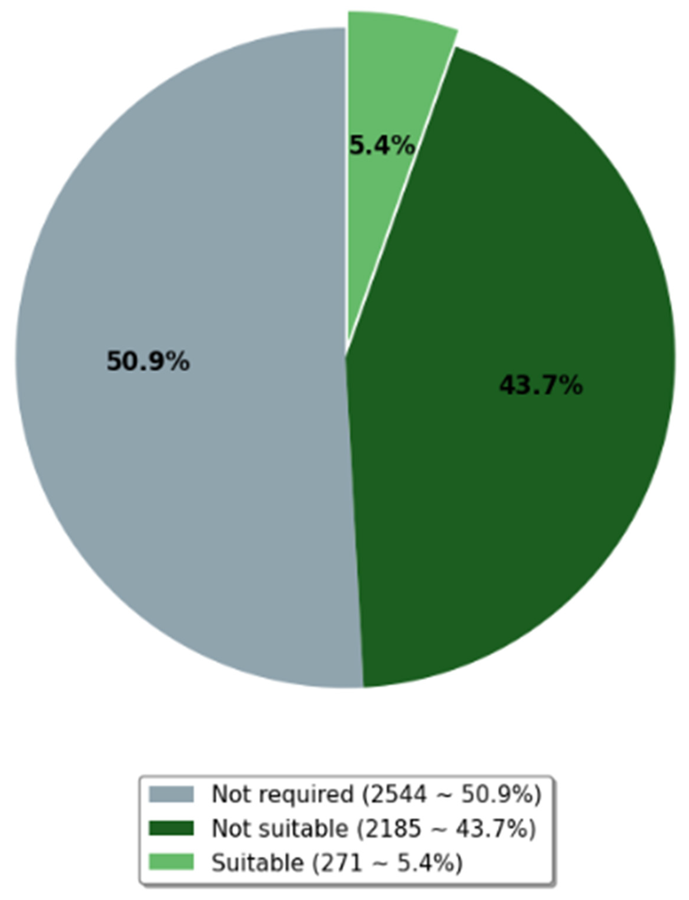
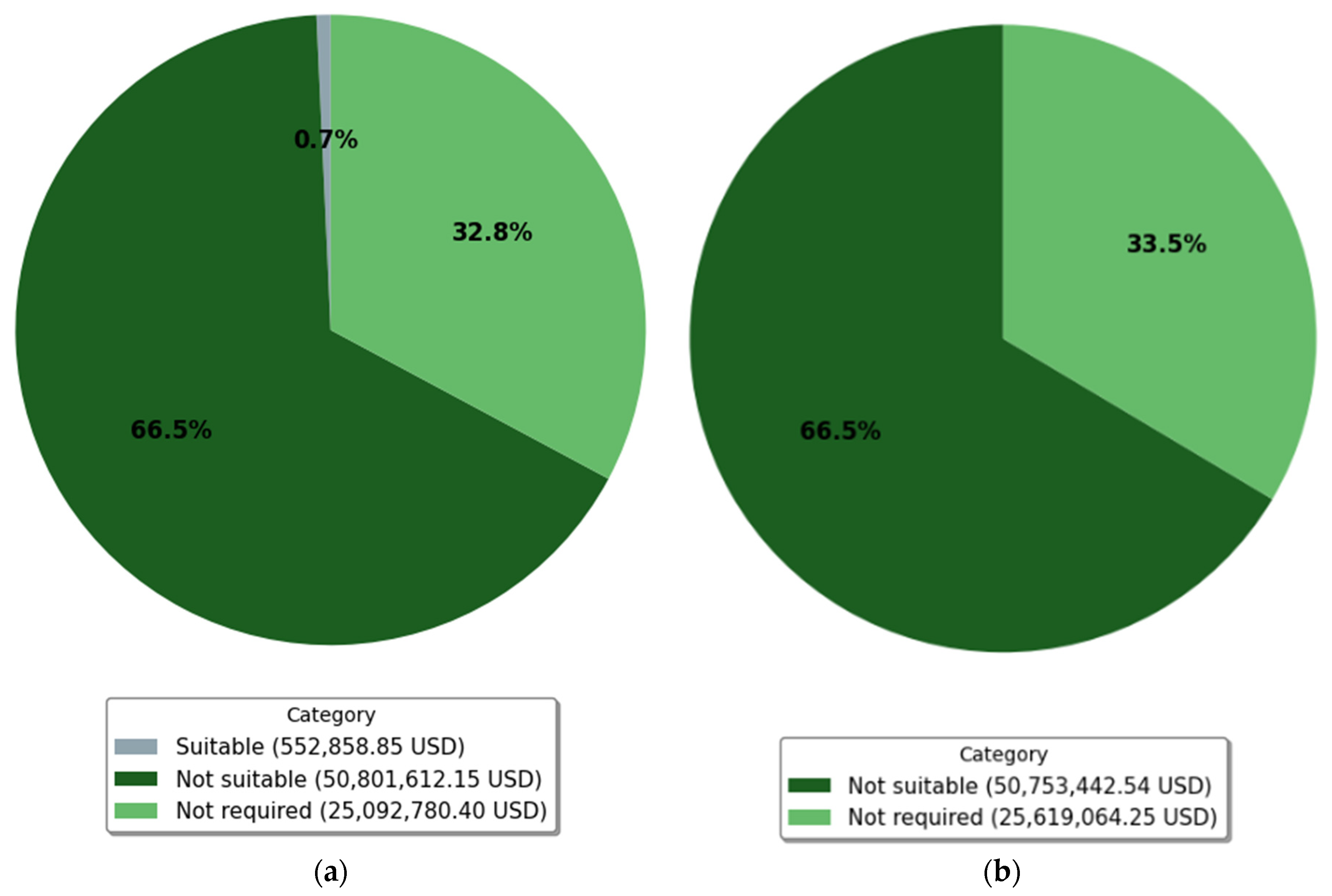
Applying the compatibility logic to the full set of 5000 real operational combinations yields the distribution displayed in Figure 2. Three categories emerge: Not required—the originally supplied inhibitor is already the most economical option meeting the 90% effectiveness threshold; Not suitable—no cheaper alternative can be adopted without compromising protection; and Suitable—a cost-effective substitute with sufficient nominal effectiveness exists. The pie chart shows that only the “Suitable” segment (dark green) offers room for cost reduction, whereas the majority of field situations fall into the other two groups.

The constructed dataset thus serves as the integral link closing the model loop: technological parameters that determine reagent demand for each asset (Table A1) form the system’s input, while commercial parameters defining the cost of meeting that demand constitute the output. The joint analysis of these arrays establishes an analytical foundation for progressing to the final research stage—the quantitative assessment of economic effectiveness achieved through adaptive redistribution of reagent resources among technologically similar assets.

3. Results

3.1. Critical Deviation Analysis

The critical deviations computed using Equation (3) for each of the eight technological parameters are presented in

Table 7. Critical deviations of parameters that preserve effectiveness at ≥90%.

Parameters	Weight, ${\mathit{\omega }}_{\mathit{i}}$	Range, ${\mathit{x}}_{\mathit{m}\mathit{i}\mathit{n},\mathit{i}}-{\mathit{x}}_{\mathit{m}\mathit{a}\mathit{x},\mathit{i}}$	$∆{\mathit{x}}_{\mathit{i}}^{\mathit{c}\mathit{r}\mathit{i}\mathit{t}\mathit{i}\mathit{c}\mathit{a}\mathit{l}}$, Absolute	$∆{\mathit{x}}_{\mathit{i}}^{\mathit{c}\mathit{r}\mathit{i}\mathit{t}\mathit{i}\mathit{c}\mathit{a}\mathit{l}}$, Relative
Temperature	0.5	40–80	8 °C	20.0%
H2S concentration	0.7	0.5–4	0.5% vol.	14.3%
CO2 concentration	0.4	0.3–1.5	0.3% vol.	25.0%
O2 concentration	0.1	0–5	5.00 ppm	100.0%
Chloride content	0.6	50–250	$33.33 \mathrm{g}{\mathrm{L}}^{-1}$	16.7%
pH of aqueous phase	0.2	5.5–7	0.75	50.0%
Flow velocity	0.4	1–5	$1.00 \mathrm{m}{\mathrm{s}}^{-1}$	25.0%
Inhibitor concentration	0.7	50–150	14.28 ppm	14.3%

, both in absolute units and as a percentage of the parameter range, clearly illustrating the “margin of safety” for each factor.

The results allow the ranking of parameters by their degree of “criticality”: the tightest operational tolerance (smallest relative critical deviation) belongs to hydrogen sulfide concentration and inhibitor concentration, both at 14.3% of their respective ranges. Chloride content follows with 16.7%, while temperature allows a 20.0% deviation. Flow velocity and CO₂ concentration share a 25.0% tolerance, and pH exhibits the widest safe band after oxygen (50.0%). The oxygen parameter, having the lowest weight (0.1), tolerates any value within the whole observed range (100%), as its influence on inhibitor effectiveness in closed systems is negligible. These results confirm that H₂S and inhibitor dosage are the most critical factors, whereas chloride content and pH have a broader operating window.

The ranking of parameters by their critical deviation reveals that H₂S concentration and inhibitor concentration have the tightest operational tolerances (14.3% of their respective ranges). This finding is consistent with well-established physico-chemical mechanisms. H₂S directly competes with inhibitor molecules for active adsorption sites on the metal surface; at elevated H₂S concentrations, the formation of iron sulfide scales can either enhance or impair protection but typically reduces the effective surface coverage of organic inhibitor films [12]. Similarly, inhibitor concentration exhibits a threshold behavior: below a critical concentration, the adsorption layer is incomplete, leaving bare metal exposed to corrosive species; above this threshold, additional dosage yields diminishing returns in protection but significantly increases cost.

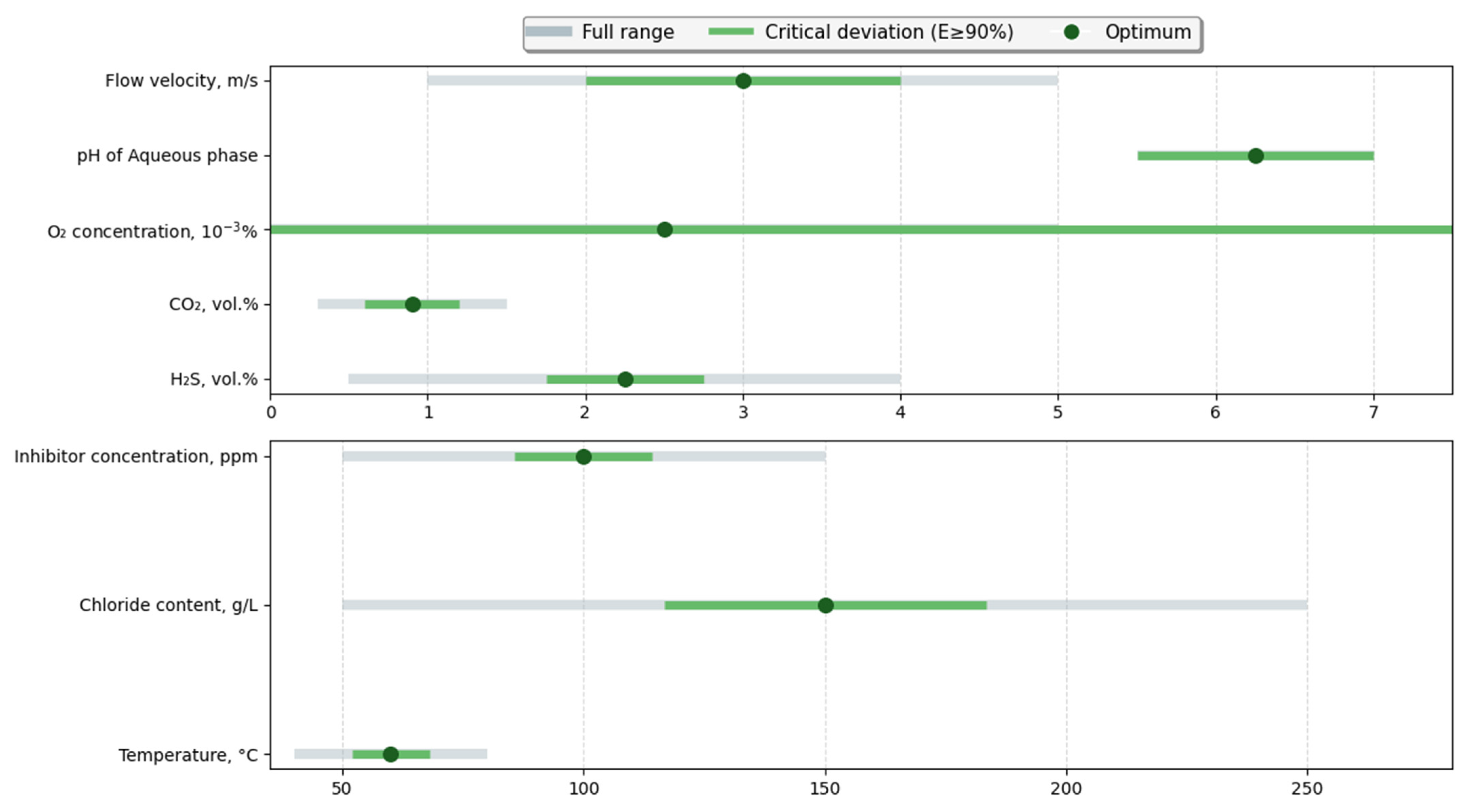
To complement the numerical data in Table 7, Figure 3 provides a graphical interpretation of the permissible deviation ranges. The light-grey bars span the full observed interval (min–max) for each technological parameter, while the green segments mark the critical deviation corridor: as long as a parameter stays within this green band, the integral effectiveness $E_{total}$ remains at least 90%, assuming all other parameters are held at their optimum. The black dots locate the optimum value itself. It is important to clarify that the term “reference point” here refers to the arithmetic mean of the parameter range, which serves as a baseline for normalization rather than a true technological optimum determined through experimental optimization. This choice is justified by standard industrial practice: when introducing a chemical reagent, an oil and gas enterprise first identifies the reagent that demonstrates the highest performance under nominal (average) conditions and only then deploys it in the field. Thus, the midpoint of the parameter interval corresponds to the conditions for which the most effective reagent has already been established. This reference point can be shifted toward the lower or upper boundary when the model is applied to assets with different operating envelopes (e.g., towards lower H₂S concentrations or lower temperatures, where inhibitor performance is typically more favorable). For a detailed justification of this approach, see Section 2.1.1. This visualization immediately distinguishes parameters with wide operating windows (e.g., pH and oxygen) from those demanding extremely tight control (e.g., CO₂ and H₂S concentrations).

3.2. Assessment of the Economic Effectiveness of the Proposed Reagent-Management Model

In the Results section, we present the economic effect obtained by shifting from a fixed (“inert”) inhibitor supply regime to an adaptive scheme that reallocates reagents among technological units that were calculated [24,25]. The methodological basis for the calculation relies on comparing annual operating costs (OPEX) under two scenarios:

• Baseline scenario (CPY_base,i)—For each technological situation, the inhibitor initially assigned in the dataset (

  Table 8. Representative results of annual operating cost calculations.

  Number	Annual Requirement, ${\mathit{M}}_{\mathit{y}\mathit{e}\mathit{a}\mathit{r}}$	Cost of Original Inhibitor	Cost per Year of Original Inhibitor	Cost per Year of Optimized Inhibitor
  4	7.6	$2700	$20,554	$17,025
  33	8.8	$2700	$23,715	$19,644
  37	9.6	$2237	$21,489	$21,489
  40	2.9	$2237	$6448	$6448
  59	5.0	$2710	$13,643	$11,260
  999	5.8	$2237	$12,949	$12,949
  1990	9.0	$2699	$24,165	$20,027
  3005	9.0	$2710	$24,448	$20,178
  4007	2.7	$2741	$7495	$6117
  4997	9.8	$2237	$21,847	$21,847

  ) is used. The cost and effectiveness of the reagent correspond to a random combination that simulates the actual presence of different lots in inventory.
• Optimized scenario (CPY_optimized,i)—For the same technological situation, from the entire pool of available inhibitors (5000 records), the reagent with the lowest unit cost is selected, provided its nominal effectiveness E_nominal is at least equal to the threshold value that guarantees the target protection level E_threshold = 90%.

3.2.1. Method for Calculating Annual Operating Costs

The economic block of the model uses the following input data:

• Daily mass flow of inhibitor $G_{inhibitor}$(kg per day), calculated for each technological combination (Table 7). This figure already incorporates dose optimization that ensures $E\ge E_{threshold}$.
• Present-value unit cost of the inhibitor (USD per ton), corresponding to a specific commercial product.
• Nominal effectiveness $E_{nominal}$ (%), indicating suitability for use under conditions demanding high protection.

The inhibitor’s daily mass flow rate (kg/day) was projected to an annual requirement by multiplying it by 365 days and converting kilograms to tons. The resulting annual mass, expressed in tons per year, was then multiplied by the unit cost (USD per ton) assigned to the given technological situation, yielding the annual operating expenditure for reagent procurement.

3.2.2. Optimization Algorithm

For each of the 5000 technological combinations, the following procedure is executed.

From the available inhibitors (Table 7) a subset of candidates is selected satisfying $E_{nominal}\ge 0.90$.

The inhibitor with the lowest unit cost in this subset is selected; its cost is $C_{min}$.

• Calculate the ${CPY}_{optimized,i}$.
• For comparison, ${CPY}_{base,i}$ corresponding to the originally assigned inhibitor in the dataset is recorded.

Thus, the optimized scenario represents a situation where the technical service, aware of the real demand and current inventory of different inhibitor grades, replaces expensive or overly effective reagents with the most economical available option without compromising corrosion-protection quality [11,22].

3.2.3. Results and Economic Effect Assessment

To evaluate the economic viability of the adaptive inhibitor redistribution strategy, annual operating costs were computed for each of the 5000 technological situations under two regimes: a baseline scenario that retains the originally assigned inhibitor and an optimized scenario that selects the cheapest admissible alternative without compromising the 90% protection threshold. The calculation procedure, detailed in Section 3.2.1 translates the optimized daily inhibitor consumption into annualized procurement costs.

A representative subset of the results is presented in Table 8, which lists ten technological combinations together with their annual inhibitor requirement, the unit cost of the originally assigned product, and the corresponding annual expenditures for both the baseline and the optimized cases.

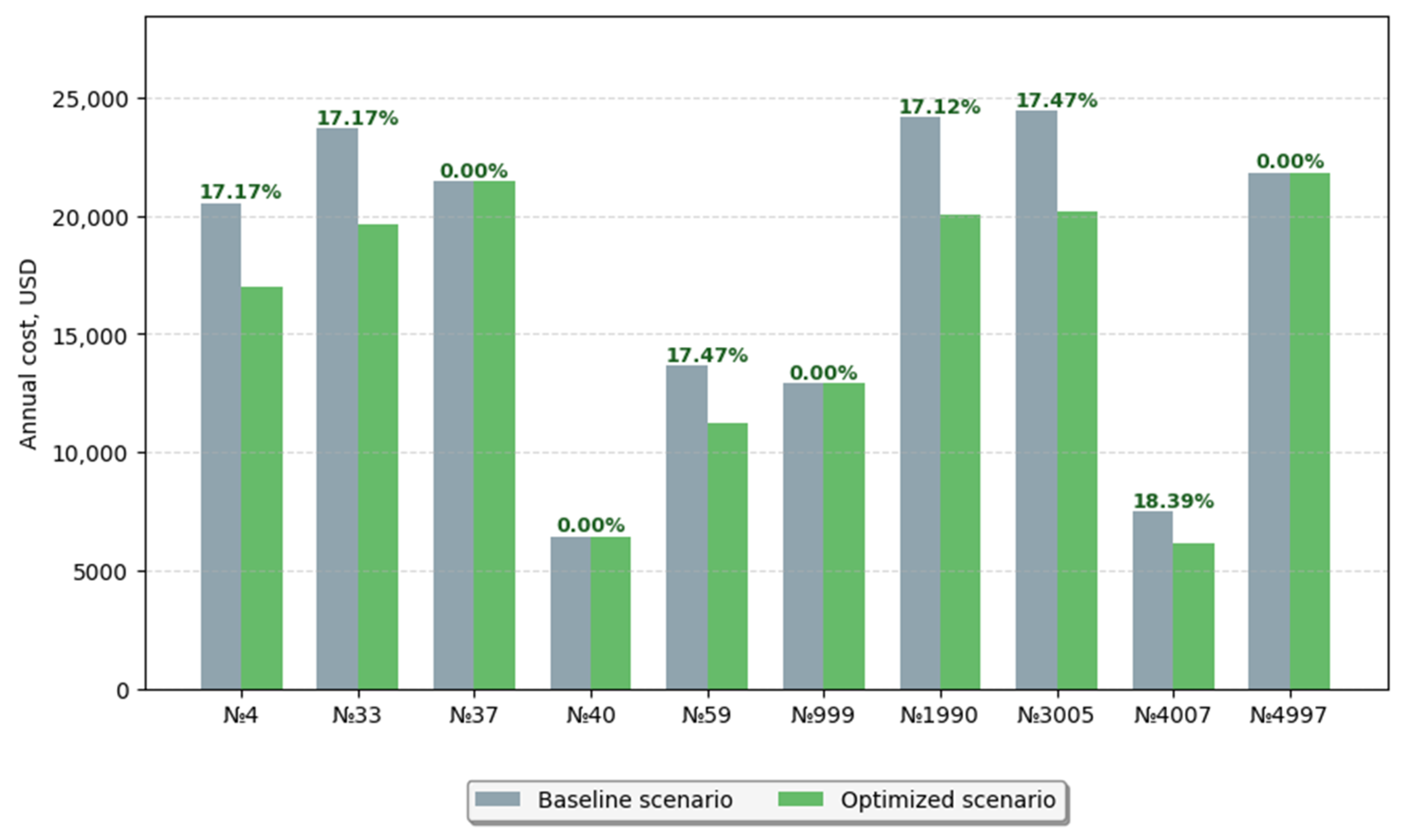
To vividly illustrate the cost reduction obtained through inhibitor substitution, Figure 4 compares the baseline and optimized annual costs for the same ten combinations in a grouped bar chart. The green bars, representing the optimized scenario, are consistently lower than or equal to the grey baseline bars. The percentage values above each pair quantify the relative savings: they reach up to 17–18% for several combinations, whereas combinations that already employed the cheapest suitable inhibitor (№ 37, 40, 999, 4997) show no change. This visualization clearly demonstrates that substantial cost savings are achievable without any loss of protective performance.

The key findings are as follows:

• Magnitude of unit effect. Relative cost reductions range from 0% (when the initial inhibitor is already the cheapest) to approximately 25% for high-cost, highly effective grades that can be replaced by more affordable analogues with sufficient protective capability. The average saving across all combinations is 0.7%.
• Integrated annual effect. Summing the annual costs of all 5000 technological units provides a holistic measure of the economic potential of the adaptive reagent-management system.

Before proceeding to the integrated indicator, it is instructive to inspect how the total annual costs are distributed among the three compatibility categories introduced earlier: “Suitable”, “Not suitable”, and “Not required”. Figure 5a,b display this distribution for the baseline and the optimized scenarios, respectively. In both charts the “Not suitable” and “Not required” categories dominate the total expenditure, but the “Suitable” slice visibly contracts after optimization, directly reflecting the savings realized in that segment.

The integrated economic effect is then quantified by Equation (9):

$$∆OPEX=\sum _{i=1}^{5000}{CPY}_{old,i}-\sum _{i=1}^{5000}{CPY}_{new,i}$$

(9)

Beyond the aggregated saving, a more detailed breakdown reveals that the economic benefit is not uniformly distributed across the 5000 combinations. Approximately 95% of the total ΔOPEX (552,858 USD) originates from 69% of the cases—those where the baseline inhibitor belonged to the highest price quartile, more than 2650 USD per ton; in contrast, combinations in which the original inhibitor already had a unit cost below 2650 USD per ton contributed about 5% to the total saving, even when a cheaper alternative existed. This finding suggests that a targeted intervention—focusing only on high-cost, overly effective reagents—would capture most of the economic gain while minimizing operational disruption.

Processing the complete dataset yields total annual inhibitor purchase costs of 80,012,389 USD under the baseline scenario and 79,459,531 USD under the optimized scenario. Consequently, the expected yearly economic benefit from implementing adaptive reagent redistribution among units with similar technological parameters amounts to 552,858 USD (expressed in 2025 prices).

4. Discussion

4.1. Comparison with Existing Approaches and Positioning of the Proposed Framework

The proposed methodology sits at the intersection of techno-economic screening, multi-criteria decision analysis (MCDA), and operational cost optimization. However, it differs from classical MCDA implementations (e.g., AHP, TOPSIS, PROMETHEE) in several respects. First, the decision criteria are not aggregated additively; instead, we employ a multiplicative product of normalized effectiveness coefficients, which reflects the compounded nature of inhibitor performance degradation—a single critical parameter falling outside its safe operating window can compromise the entire protection system. Second, the weight coefficients are not normalized to unity, which preserves their physical interpretation as sensitivity multipliers rather than probability-like importance scores. Third, the model is explicitly designed for operational screening, where the decision space is constrained to an existing inventory of already approved reagents and where the primary objective is rapid cost-saving identification rather than comprehensive life-cycle optimization.

In contrast to conventional TEA and LCCA studies, which typically assess a single project or asset over its entire lifespan, our approach evaluates the reallocation of chemicals across multiple assets within a single planning horizon (annual procurement cycle). The economic block is directly fed with real purchase prices extracted from actual tenders (2020–2025), ensuring that the output reflects current market volatility. This makes the model particularly suitable for supply-chain management in large oil-and-gas holding companies, where reagents are frequently procured in bulk and distributed among subsidiaries.

4.2. Interpretation of Results and Advantages of the Approach

In the contemporary industrial economy, multidisciplinary cost-management approaches are increasingly relevant. The integrated model presented here synthesizes technical–economical analysis (TEA), life-cycle cost assessment (LCCA) and multi-criteria decision-making (MCDA). This methodological blend moves beyond conventional accounting for direct costs, providing a comprehensive evaluation of technological effectiveness in conjunction with environmental and economic factors [23,24]. The study is grounded in an extensive dataset comprising 5000 combinations of real field parameters. During validation, 271 parameter sets—corresponding to the “Suitable” category in Figure 5—were identified as meeting the key criterion of adaptive reagent transfer feasibility. Quantitative analysis demonstrates that even under constrained applicability of flexible dosing schemes, operational cost optimization yields a significant reduction in annual expenditures [13,25]. The achieved savings of 552,858 USD, reflected in a 0.7% reduction in annual operating costs (CPY), confirm the model’s validity and its high practical potential for the real sector. The model is built on principles of universality, making it applicable to a wide range of oil-and-gas assets. A critical prerequisite for correct functioning is the formalization of input parameters that determine reagent efficacy. These include thermodynamic indicators (temperature), concentrations of aggressive constituents (H₂S and CO₂), and hydrodynamic flow characteristics—in total, eight key variables. The mathematical model incorporates a weighting mechanism for these parameters, with weight coefficients subject to iterative adjustment as empirical data accumulate, thereby enhancing predictive accuracy in assessing actual reagent performance.

Beyond the immediate goal of reducing operating expenses, the developed toolkit acquires strategic importance within supply-chain management [26,27]. Market conditions are characterized by high uncertainty: production discontinuation of specific reagent lines or exit of manufacturers can narrow the competitive base. The integrated model enables rapid simulation of how such market fluctuations affect overall economic outcomes. In the event of price increases or shortages of a particular product, the system automatically adapts the dosing strategy, switching to alternative, more cost-effective reagents without compromising required protection levels. Thus, the model serves not merely as a calculation tool but as a flexible mechanism for adaptive management of production inventories amid market volatility.

4.3. Reducing Environmental Impact Risks

Adaptive management of the reagent inventory can substantially reduce ecological costs in the oil-and-gas sector. Each corrosion-inhibitor formulation, scale-preventing agent, biocide, etc., contains a unique combination of active substances that, when dosed correctly, lowers concentrations of toxic compounds (sulfates, chlorides, and heavy metals) in the working environment [28,29]. For instance, amine-based inhibitors form complex ions that do not enter the oil phase and thus do not pollute water bodies.

Economically justified allocation of reagents across assets diminishes the risk of equipment overload, thereby reducing the likelihood of sudden failures and spills. Switching to an optimized dosing regimen extends the service life of corrosion-resistant equipment, lowering the probability of pipeline or tank leaks.

The benefits of operational management are evident: fewer incidents and spills, cost savings from mitigated consequences, and enhanced corporate reputation as a responsible environmental steward. Ultimately, the adaptive system delivers not only financial gains (OPEX reduction of 0.7%) but also a sustained decrease in pollution risks, making it a valuable tool for strategic planning in the oil-and-gas industry.

4.4. Limitations and Future Directions

The proposed methodology offers an integral approach to valuing chemical reagent use in the oil-and-gas sector based on TEA, LCCA and MCDA. Although widely applicable, the model has inherent limitations that must be consciously considered when interpreting results and implementing it operationally. Transferring a specific chemical composition from one asset to another requires adherence to a set of technological, geological and infrastructure parameters [30,31]. The model incorporates eight key variables (temperature, H₂S, CO₂, O₂, mineralization, pH, flow velocity, and inhibitor concentration). Any deviation from the optimal value of one of these parameters reduces protective effectiveness and, consequently, increases costs. Therefore, transferring a reagent necessitates a separate regression analysis for each “asset-product” pair, considerably complicating practical implementation [32,33].

Moreover, the economic efficiency calculated within this methodology is based on total expenditures across all assets included in the analysis (Table 4). When expanding the asset portfolio, the model retains linearity only under the assumption of homogeneous technological regimes and comparable environmental parameters [34,35,36]. In practice, peripheral fields with unique geological characteristics often exhibit effectiveness coefficients that differ markedly from the averages used in the model, leading to bias in OPEX and NPV estimates.

5. Conclusions

This study presents a screening-level methodology for the economic justification of inhibitor selection and reallocation across oil and gas assets. The proposed model integrates eight key technological parameters—temperature, H₂S concentration, CO₂ concentration, O₂ concentration, chloride content, pH of the aqueous phase, flow velocity, and inhibitor concentration—with actual procurement prices (2020–2025) to identify cost-effective substitution opportunities without compromising the required protection effectiveness. The core of the methodology is a multiplicative screening model based on normalized dimensionless effectiveness coefficients and parameter-specific weights, combined with the concept of critical deviation thresholds that quantify the maximum permissible drift from the reference operating point while maintaining the target protection level of 90%.

The main findings can be summarized as follows.

Economic potential: The economic optimization, grounded in real procurement data, demonstrated that annual operating costs (OPEX) for inhibitor procurement can be reduced by 552,858 USD (approximately 0.7% of total reagent procurement costs) through adaptive reallocation of inhibitors among technologically similar assets. Relative cost savings per technological combination range from 0% (where the initially assigned inhibitor is already the most economical) to approximately 25% for high-cost, highly effective grades that can be replaced by more affordable analogues with sufficient protective capability. Notably, 95% of the total savings originate from 69% of the cases—those where the baseline inhibitor belonged to the highest price quartile (>2650 USD per ton)—suggesting that targeted intervention on expensive reagents captures most of the economic gain.

Environmental implications: By enabling more precise dosing and reducing the likelihood of incidents associated with improper reagent selection—such as accelerated corrosion, equipment failure, and spills—the adaptive management of the reagent inventory contributes indirectly to reducing environmental pollution risks. The model supports the selection of reagents with lower ecotoxicological impact by incorporating environmental criteria alongside technological and economic factors.

The proposed methodology is designed as a practical tool for petroleum engineers, procurement specialists, and corrosion management teams, enabling rapid, data-driven decisions in chemical inventory management. Its modular structure allows for iterative calibration of weight coefficients as field data accumulate, making it adaptable to diverse operating conditions across different subsidiaries of oil and gas holding companies. Unlike traditional MCDA approaches that require static weight normalization, our multiplicative framework preserves the independent physical nature of each parameter and allows individual weights to be adjusted without affecting the relative importance of others.