Article

Steady-State Modeling of a Natural Convection-Driven, Condensing Methanol Reactor

1
Brusche Process Technology B.V., Twentepoort West 29, 7609 RD Almelo, The Netherlands
2
Sustainable Process Technology, Faculty of Science and Technology, University of Twente, P.O. Box 217, 7500 AE Enschede, The Netherlands
*
Authors to whom correspondence should be addressed.
ChemEngineering 2026, 10(5), 62; https://doi.org/10.3390/chemengineering10050062
Submission received: 20 March 2026 / Revised: 30 April 2026 / Accepted: 7 May 2026 / Published: 12 May 2026

Abstract

In this paper, a flexible steady-state model of a highly integrated, natural convection-driven condensing methanol reactor was developed. The flowsheet model includes 1D submodels of the different sections of the integrated reactor–condenser and includes a method to estimate the maximum possible natural convection-driven flow. Experimental data are used to create a shortcut description for the heat transfer coefficients in the model. The model results indicate that when heat losses can be mitigated, autothermal operation is possible. The major part of the heat integration takes place in the economizer section; however, a significant amount of heat transfer occurs at the catalyst bed also. The model predicts that the loop mass flow and single-pass conversion strongly depend on the catalyst bed inlet temperature. Experimentally measured catalyst preheater and condenser duties suggest, however, that the model-calculated mass flow is likely too low and that it is less dependent on the catalyst bed inlet temperature than the model predicts. A possible cause for this is the neglect of radial temperature gradients in the catalyst bed in the model, overestimating the conversion. Another possible cause is a measurement error in the bed inlet temperature, causing the actual temperature to be lower than the measured value. Natural convection calculations show that the maximum achievable flow strongly depends on the single-pass conversion and that given a single-pass conversion, a minimum temperature difference is required for flow in the right direction. Sensitivity analyses (neglecting heat losses to the environment) show that with the current heat transfer description, the feasible operating range for autothermal, natural convection-driven flow is sizeable. However, at lower recycle mass flows, heat transfer is too fast, leading to premature condensation in the economizer section. If the heat transfer coefficient is smaller than the currently predicted value, autothermal operation is possible in a wide range of conditions. If heat losses are mitigated, the maximum productivity of 2000 kg MeOH m cat . 3 h 1 is achievable at high pressure, a moderate catalyst bed inlet temperature and a low condenser temperature.

1. Introduction

It is widely accepted that methanol can play an important role as a chemical intermediate and medium for energy storage in the chemical industry of the future [1,2,3]. This is because methanol can be made selectively from CO2 [4] (possibly produced via direct air capture) and hydrogen (made via the electrolysis of water with green electricity), is a relatively safe, easily stored and transported liquid at ambient conditions, and can be converted to a wide range of chemicals [1,3,5]. Methanol can also be converted to electricity in a fuel cell and thus has potential application as a large-scale energy storage medium [6]. Finally, methanol has a high hydrogen density and can be converted back to hydrogen and CO2 relatively easily, making it a candidate for hydrogen storage and transportation [7].
The synthesis of methanol traditionally uses CO-rich synthesis gas, which is a process that is over a century old [8,9]. It is, however, possible to use the same catalyst to convert CO2-rich syngas to methanol as well [10]. The equilibrium conversion is significantly lower when starting from CO2-rich synthesis gas (20–25% when starting from CO2 as opposed to 60–70% when starting from CO under typical operating conditions). This means that in a conventional chemical process, methanol synthesis from CO2 requires a large gas recycle with the associated large equipment volumes and compressors. Furthermore, water is produced as a by-product when starting from CO2, leading to a much higher water partial pressure during the reaction, which negatively affects the catalyst stability and lifetime [11,12,13].
Several approaches are investigated to solve these challenges, ranging from electrochemical [14,15,16,17] and photochemical processes [18,19] to thermochemical processes using innovative reactor designs. The former two technologies are still in the development phase, and more research is required before it can be applied commercially [14,16,18]. In the thermochemical processes category membrane reactors [20,21,22,23,24], sorption-enhanced reactors [25,26,27,28] and condensing methanol reactors [29,30,31] have been developed. The membrane and sorption-enhanced reactors are appealing, since they remove water in situ, driving the equilibrium further toward the product side and positively affecting catalyst stability by lowering the steam partial pressure. However, the selectivity and long-term stability of the membranes and scaling up of the process are still challenges to be solved [32], and the operation of a sorption-enhanced reactor is significantly more complex than a traditional reactor due to the dynamic nature of the adsorption processes and the fact that sorbents are not perfectly selective [25]. The condensing methanol reactors are therefore especially interesting, as they are simple in construction and operation (requiring no membranes or sorbents). In a condensing methanol reactor, the products are condensed inside the reaction vessel either by using very high pressures to promote condensation at the catalyst bed [33,34] or by locally lowering the temperature and condensing the products in a separate section [30,31]. While both approaches can lead to near 100% yields over the whole reactor, this last approach is better for the stability of the catalyst [13,33].
In the work of van Schagen et al. [31], the experimental setup of a highly integrated, natural convection-driven condensing methanol reactor was discussed and successfully demonstrated. In this reactor, CO2 is hydrogenated to methanol and water over a commercial Cu/ZnO/Al2O3 catalyst. The methanol and water produced are condensed by locally lowering the temperature and removed as liquid. The unconverted gases are internally recycled, allowing for a near-100% yield of methanol. By placing the warm catalyst bed in the bottom of the reactor and the cool condenser at the top, a driving force for free convection gas circulation is generated so that the reactor can operate without any moving parts. Furthermore, internal heat integration between the hot catalyst outlet stream and the cold gas recycle is targeted to realize operation without any external heat input (so-called autothermal operation). Finally, the reactor concept has been designed and proven to operate intermittently, dealing with fluctuations in the available feedstock internally without requiring large buffers for the feedstocks or energy. This makes the concept well suited for decentralized operation on renewable energy sources [35,36] or for chemical energy storage [2].
For details about the reactor design, the reader is referred to van Schagen et al. [31], but the design is briefly summarized here. The major part of the reactor is essentially a vertical tube-and-shell heat exchanger (with seven 1” tubes with a length of about 1.5 m placed in a unit cell configuration). The catalyst bed is located in the bottom part of the seven tubes. Just before the catalyst bed in each tube, an electrical heating element is placed for start-up purposes. Above the tube and shell sections, a condenser section is located in which the products are condensed using a water-cooled, finned condenser.
The reactor operation was successfully demonstrated in the work of van Schagen et al. [31], but for further design purposes, interpretation of the experimental results, sensitivity analyses, and scaling up, it is imperative to have a reliable steady-state model of the system. While there are many studies on the steady-state modeling of the processes using commercial flowsheeting tools [37,38,39,40,41] or detailed studies on modeling the catalyst bed [42,43,44], the integrated nature of the reactor studied in this paper requires an integrated model describing heat and mass transfer in the various parts of the reactor as well. Furthermore, traditional flowsheeting programs are not able to calculate the circulation flow in the system that is driven by natural convection. The magnitude of the circulation flow is determined by an intricate balance between density differences in the system (in turn, affected by heat transfer and reactant conversion) and friction in the system. The circulation flow subseqently affects the reactor performance (single-pass conversion and heat transfer), meaning that a highly integrated model is required to describe these effects. The objective of this paper is therefore to develop and explore a steady-state model of the reactor. The model should be modular, working with unit operations connected by streams, which is similar to conventional flowsheeting tools to allow the rapid exploration of alternative designs. The customizability of the model is also required to be able to implement, for example, the internal heat integration and free convection flow calculation in the model. Furthermore, it is desirable if the model is sufficiently fast so that sensitivity analyses can be conducted in reasonable time.
First, the structure, numerical methods and model details are discussed. Special attention is given to the calculation of the maximum achievable natural convection flow in the reactor and the calculation of heat transfer coefficients for use in the model from the experimental data. Second, the model results are discussed, beginning with the comparison of experimental data to the model results and the prediction of several key performance indicators (like single-pass conversion and energy flows) by the model. Then, some more attention is given to the natural convection flow phenomena in the setup and the prediction thereof by the model. Finally, the model is used to carry out sensitivity analyses on the operating pressure, catalyst bed inlet temperature and condenser temperature. From these sensitivity analyses, a viable operating range is determined in which natural convection-driven autothermal operation is possible.

2. Modeling Methods

The goal of the model in this paper is to describe the steady-state experimental results of the experimental setup of van Schagen et al. [31] and to conduct sensitivity analyses on the setup operating and design parameters. First, the general model structure is explained, including its flowsheet. Some details are given on the numerical methods employed in the model solution. A shortcut method is then discussed to calculate the maximum achievable natural convection flow in the setup. The heat transfer description in the model and the input of experimental data to the model is then discussed, and finally, the model assumptions and limitations are discussed.

2.1. General Model Structure

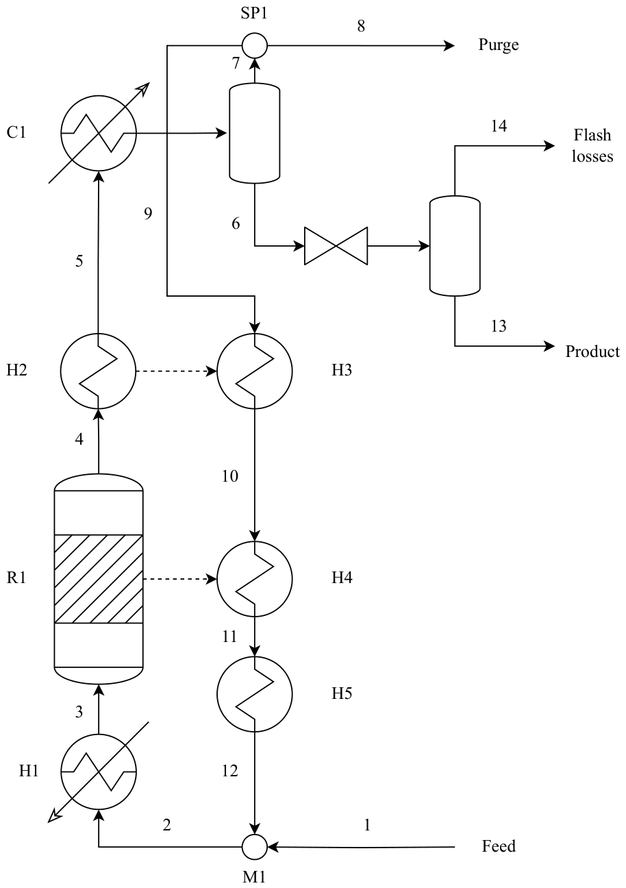
The basis for the model is the experimental setup whose details are given in van Schagen et al. [31]. The actual P&ID of the setup is simplified to the flowsheet in Figure 1. The feed (with the correct CO2/H2 ratio, pressure and temperature) enters the reactor via stream 1. Then, it is mixed with the recycle in M1. The combined stream is preheated with heater H1 (corresponding to electrical heating elements placed before the catalyst bed in the actual reactor) before being sent to the catalyst bed (R1). The heat integration zone consists of H2 and H3, where heat flows from the catalyst bed outlet stream to the recycle stream. The condenser (C1) follows after H2, and after that, the liquid product stream is flashed at atmospheric pressure. The gas recycle (stream 7) passes splitter SP1, where a small purge is installed to help the model converge. The recycle then passes H3 and H4, where heat from the tube side and catalyst bed heats up the recycle stream. H5 is a heater that can be used to model heat losses to the bottom flange of the reactor.
In the model, H3 (see Figure 1) is modeled as a utility heater with a constant outlet temperature. R1 is a 1D, plug flow reactor of which the energy balance is also modeled along with heat exchange to the shell side (to H4). Note that R1 and H4 form together the tube and shell sides of a single heat exchanger. To calculate the reaction kinetics, the 6-parameter model by Slotboom et al. is used [45]. H2 is modeled as a counter-current tube-and-shell heat exchanger together with H3 in which H2 indicates the tube side and H3 indicates the shell side. The flow profile is assumed to be plug flow in these units. C1 is modeled as a 1D plug flow condenser where heat is withdrawn from the process stream with cooling water. After the condenser, the liquid product stream is split off and flashed in an adiabatic flash. In H3 and H4, heat losses to the environment can be included by specifying the heat transfer coefficient and environmental temperature. H5, finally, is a utility heater with a constant outlet temperature that can be used to account for additional heat losses in the bottom flange of the reactor. More information on the details of the individual unit operation models is given in Section S8 in the Supplementary Information.
The steady-state model is fully implemented in Python (version 3.12.7) and is built up of units (corresponding to various unit operations) that are connected by streams (see Figure 1), which is akin to well-known flowsheeting tools used throughout the industry and academia. The modified Soave-Redlich-Kwong (SRK) equation of state proposed by Mathias [46] with the parameters by van Bennekom [33] is used as the thermodynamic model. Several types of units are implemented, including utility heaters, two-stream heat exchangers, kinetic and equilibrium reactors in 1D and 2D, both isothermal and non-isothermal, condensers, flashes, compressors and a shortcut distillation column. The model is able to apply heat integration between the catalyst bed and a process stream both co- and counter-currently. The implementation of the model in Python makes it easy to use and trivially customizable while still relatively fast (by leveraging NumPy). This is a major advantage in modeling a highly integrated non-typical system like the reactor studied in this paper. In the model, it is also trivial to add/remove units and streams and change the order of unit operations. This is useful for investigating different reactor configurations and scaling up. The model is able to automatically resolve the calculation order of the flowsheet and iteratively solve recycles. Using a shortcut method, the model is also able to estimate the maximum possible natural convection recycle given the conditions in all unit operations. The thermodynamics and physical property engine of the model is implemented in C++ to allow fast calculations, but it is useable from Python. Details about this engine are given in Sections S2 and S3 in the Supplementary Information.

2.2. Numerical Methods

In the model, the reactor (R1/H4), economizer (H2/H3) and condenser (C1) are plug flow units which require a set of differential equations to be integrated. Because all units are modeled in 1D and no axial dispersion of heat and mass is taken into account, this results in an initial value problem for all units. Some units (like the condenser) require a set of differential algebraic equations to be solved; for these units, the IDA solver from the SUNDIALS suite is used [47,48]. For the other units, the CVode solver, also from the SUNDIALS suite, is used. Calculation loops (recycle streams and heat integration loops) are iteratively calculated using a direct substitution method until the desired tolerance is met (typically a relative error in the mass and energy balances of 1 × 10⁻⁵). More details are given in Section S8 in the Supplementary Information.

2.3. Natural Convection Modeling

One particular objective for the model is to estimate the maximum recycle flow rate in the reactor that can be achieved with natural convection. To this end, a simple approach based on the 1D momentum and continuity equations is used [49]. The steady-state 1D momentum and continuity equations are given in Equations (1) and (2). Here, u is the axial velocity, ρ is the fluid density, p is the pressure, g is the gravitational constant, φ is the angle between the direction of the gravity force and the fluid flow, τ is the shear stress (friction), r is the tube radius and z the coordinate in the loop. Note that the physical properties and state variables are dependent on the location inside the reactor.
ρ u 2 z = p z + ρ g cos φ 2 τ r
ρ u z = 0
Realizing the flow path through the reactor is a loop, integrating Equations (1) over the loop and using the fact that the pressure and velocity at z = 0 and z = L are equal (since the loop is closed) yields the following:
ρ u 2 z = L ρ u 2 z = 0 = p z = L p z = 0 + 0 L ρ g cos φ d z 2 0 L τ r d z
0 = 0 L ρ g cos φ d z 2 0 L τ r d z
In the horizontal sections of the loop, gravity does not play a role (it only plays a role in the vertical tube and shell sides of the reactor); thus, it makes sense to split the buoyancy force integral in two parts corresponding to the vertical sections of the reactor. The friction integral can also be split between the catalyst bed (most likely the major contributor to the friction, verified later) and the remainder of the reactor. This leads to
0 H ρ shell g d z 0 H ρ tube g d z = 2 0 L cat . τ cat . r d z + 2 L cat . L pipe τ pipe r d z
Here, H is the height of the setup, ρ shell is the density in the shell side, ρ tube is the density in the tube side, L cat . is the length of the catalyst bed, and L pipe is the length of the loop where no catalyst bed is present. Using the Stokes–Ergun equation (from Pope et al. [50] that is better able to describe the low-velocity regime than the conventional Ergun equation) to calculate the friction in the catalyst bed and the Darcy–Weisbach equation for the rest of the loop yields the following [51]:
0 H ρ shell g d z 0 H ρ tube g d z = 0 L cat . ρ u s 2 1 ε f p d p ε 3 d z + L cat . L pipe ρ u 2 f D 2 D d z
Here, u s is the superficial velocity in the catalyst bed, ε is the bed porosity, f p is the Stokes–Ergun friction factor, d p is the catalyst particle diameter, f D is the Darcy friction factor and D is the hydraulic diameter. Note that the constants in the Stokes–Ergun equation were refitted to experimental data of the pressure drop over the catalyst bed to improve the correlation predictions (see Section S7 in the Supplementary Information). Finally, assuming that the friction in the catalyst bed is much larger than in the rest of the loop (justified because the friction in the catalyst bed at typical operation conditions calculated with the refitted Stokes–Ergun equation is in the order of 100 Pa and the friction in the rest of the piping in the setup calculated by the Darcy–Weisbach equation accounting for bends and sudden size changes using the equivalent length method [52] is less than 10 Pa due to the low velocities in the system) and introducing the mean densities on the tube and shell sides ( ρ ¯ = 1 L 0 L ρ d z ) of the reactor yields the following:
g H ρ ¯ shell ρ ¯ tube = L cat . ρ ¯ gas , cat . u ¯ s 2 1 ε f p d p ε 3
Once the temperature, pressure and composition profiles are calculated with the steady-state model, Equation (7) can be solved numerically for the superficial velocity (and in turn the mass flow). Because of the assumptions made in the derivation of Equation (7), this gives an upper bound on the achievable natural convection mass flow. In reality, the maximum flow will be slightly lower because of, for example, radial temperature gradients, additional friction in bends and diameter changes in the reactor, which are not taken into account here.

2.4. Model Input Data and Heat Transfer Description

In addition to the geometrical parameters, which can readily be inserted into the model, there are some other parameters required to run the model. Operational parameters, like pressure, feed flow, composition, temperature, catalyst bed inlet temperature (=H1 outlet temperature) and condenser temperature can be obtained from experimental data (when comparing the model to an experiment) or varied in a sensitivity analysis. An overview of the parameters used in the simulations is given in Table 1. Other parameters, notably heat transfer coefficients, cannot directly be influenced in the setup, and their values cannot be easily obtained from the experimental results. Due to local natural convection effects induced by local temperature gradients inside the tubes and inside the shell, heat transfer coefficients are expected to be different than what the standard literature correlations predict. To accurately simulate how the reactor will perform under varying conditions, an adequate description for the heat transfer coefficients is required.
The most straightforward solution would be to fit the heat transfer coefficients from the catalyst bed to the shell side and in the heat-integration zone so that the model-predicted temperature profiles match the experimental ones. However, based on Computational Fluid Dynamics (CFD) results and experimental insights not discussed in this manuscript, it is expected that the heat transfer coefficient is not constant over the length of the reactor. This is mainly because of local gas circulation effects and the definition of the driving force [53]. Capturing this heat transfer coefficient profile in a likely setup specific correlation leads to a lot of fitting parameters, which is undesirable. An alternative approach is therefore proposed. It is already assumed that the flow in the tube and shell sides of the reactor is plug flow. For this case, the energy balance in the tube side is formulated in Equation (8). Here, m ˙ is the mass flow, C p is the heat capacity, T is the tube-side temperature, z is the axial coordinate, A cs is the cross-sectional area of the tube side, a wall is the specific surface area for heat transfer, U ov is the overall apparent heat transfer coefficient and T shell is the shell-side temperature.
m ˙ C p d T d z = A cs a wall U ov z T z T shell z
A cs and a wall can be calculated from the reactor geometry. When the model is run, C p is calculated using the model-predicted composition and temperature. This is also the case for m ˙ , which is an output of the model (mainly depending on the single-pass conversion calculated by the model). The temperature gradient d T d z and temperature difference can be calculated from the experimental data and interpolated to the axial grid points the model uses. The only unknown left is the overall apparent heat transfer coefficient U ov z which can now be calculated at every axial coordinate. Using Equation (8) therefore allows the heat transfer coefficient profile to be calculated from the experimental data without any fitting. The same approach is used to calculate the apparent heat transfer coefficient for heat losses from the shell side to the environment. For the heat transfer coefficient from the catalyst bed to the shell side, this approach is less convenient because the temperature profile in the catalyst bed is unknown, so this coefficient is simply fitted so that the bed outlet temperature in the model matches the experimental value. Finally, by using this approach to calculate the heat transfer coefficients for many experiments, a correlation for the different coefficients as a function of the mass flow can be fitted.

2.5. Model Assumptions and Limitations

In the development of the model in this paper, several assumptions are made, which are discussed here. First of all, the different parts of the reactor are modeled using steady-state, 1D plug-flow models, as discussed before. The use of 1D plug-flow models leads to an efficient implementation of the model that can be solved rapidly (see Section S10 of the Supplementary Information), but they are of course a simplification of reality. This should be kept in mind especially when using the model for scaling up the system. The effect of 2D heat transfer on the catalyst bed is investigated in this paper (see Section S12 in the Supplementary Information and Figure 9) and is shown to be important. Furthermore, 2D and transient effects on heat transfer in the economizer section are studied in Chapter 6 of van Schagen et al. [53] and shown to be of significant influence as well. However, incorporating such effects in the present model would make it much more complex and slow. Since the current model is able to predict experimental trends well while still being relatively simple and fast, it achieves a good compromise between accuracy and complexity.
Heat transfer between different parts of the reactor and between the reactor and the environment are accounted for using an overall heat transfer coefficient formulation. For the experimental data comparison, these heat transfer coefficients are calculated from the experimentally measured temperature profiles, as discussed in the previous section. During the sensitivity analyses, the heat transfer coefficients are calculated with linear correlations fitted to the experimental data, whose parameters are shown in Table 2. It must be noted that these correlations are specific to this setup and not fitted in a dimensionless form due to limitations in the available data from the setup, so their results cannot readily be extrapolated to a system with different dimensions. When calculating the operability range (Section 3.6), heat losses to the environment are neglected. More details about assumptions in the different parts of the model are discussed in Sections S2, S3 and S8 of the Supplementary Information.

3. Results and Discussion

First, the model is compared with and validated against experimental data. The model requires a description for its heat transfer coefficients, which are fitted to experimental data using the shortcut method as described above. The model is subsequently used to predict quantities like the single-pass conversion, recycle flow rate and energy flows for the different experiments that were run. Then, the natural convection behavior in the setup as a function of the tube and shell sides’ temperature difference and single-pass conversion is investigated more closely. Finally, sensitivity analyses are conducted with the model on key operating parameters like the pressure, catalyst bed inlet temperature and condenser temperature. An overview is made of the range in which autothermal, natural convection-driven operation is possible as a function of the different operating parameters.

3.1. Model Validation

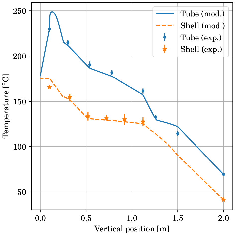
The different parts of the model (e.g., the thermodynamic engine, physical property engine, reactor models, condenser model, etc.) are validated separately against experimental data to verify their correct implementation. Details are discussed in Section S7 of the Supplementary Information. In van Schagen et al. [31], the experiments run with the condensing methanol reactor setup are described. Here, these experimental results are compared to the steady-state model output. First, the heat transfer behavior is investigated. Figure 2 shows the model-predicted temperature profiles in the tube and shell sides of the reactor (solid and dashed line) and compares this to the experimental data (points) for the experiment at 60 bar and a catalyst bed inlet temperature of 220 °C. The agreement in tube-side temperature is good with the temperature profile both matching the shape of the experimental temperature profile as well as the absolute value. For the shell side, there is also a good agreement in the trend and absolute value of the temperatures. This shows that the approach for calculating the local heat transfer coefficients works well.
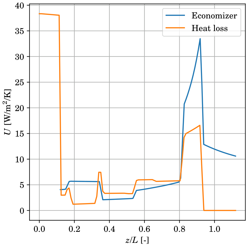
Figure 3 shows the calculated apparent heat transfer coefficient profiles for the experiment at 60 bar and a catalyst bed inlet temperature of 220 °C. Looking at the trend in the heat integration (economizer) section, it is clear (from the high heat transfer coefficient and rapidly decreasing temperature) that a lot of heat is heat integrated near the end of the tube side. Here, the shell diameter increases slightly, causing a change in flow profile and influencing the heat transfer coefficient. In the central section, the heat transfer coefficient is very low (apparently around 5 W m−2 K−1)—much lower than would be expected for typical convection through a pipe at the same mass flow and hydraulic diameter (around 35 W m−2 K−1 for laminar forced convection [54]). This low heat transfer coefficient is likely caused by local natural convection effects. The apparent heat loss heat transfer coefficient follows a similar profile, starting very high at the catalyst bed, then decaying toward the central section, and increasing again at the top of the tube and shell sections. The high value of the loss coefficient at the catalyst bed can be explained by the proximity of this section to the uninsulated steel bottom flange, allowing for large heat losses there. The jagged profiles in Figure 3 are caused by the linear interpolation of the experimental temperature profiles when calculating the heat transfer coefficients.
The trends in Figure 2 show that the tube-side temperature initially rises quickly because of the catalyst bed preheaters. Then, the exothermic reaction causes the temperature to rise even further, after which heat transfer to the shell side lets the gas temperature decay again, causing the outlet temperature of the catalyst to be lower than the inlet temperature. At the end of the tube side, in the section between the tube-side outlet and the condenser inlet, there is also significant heat loss. Looking at the shell-side temperature profile (from right to left), at the top of the tube and shell sections, the shell-side temperature rises very quickly and then stays constant for a certain amount of length. This could indicate that significant mixing happens in the shell side of the reactor (which is not included in the model), leading to the near uniform temperature. Another explanation is that the heat losses to the environment are approximately equal to the heat integrated in the section where the shell temperature is constant. Finally, as the gas in the shell approaches the catalyst bed, the temperature rises further, indicating a significant amount of heat transferred from the bed to the shell-side gas.
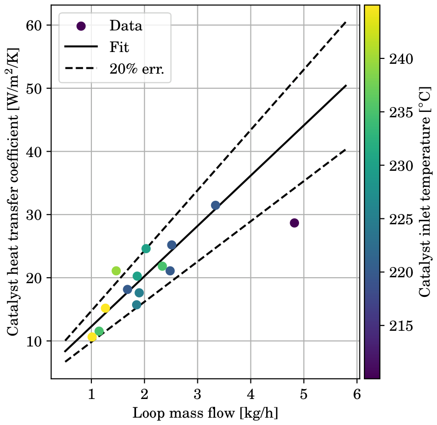
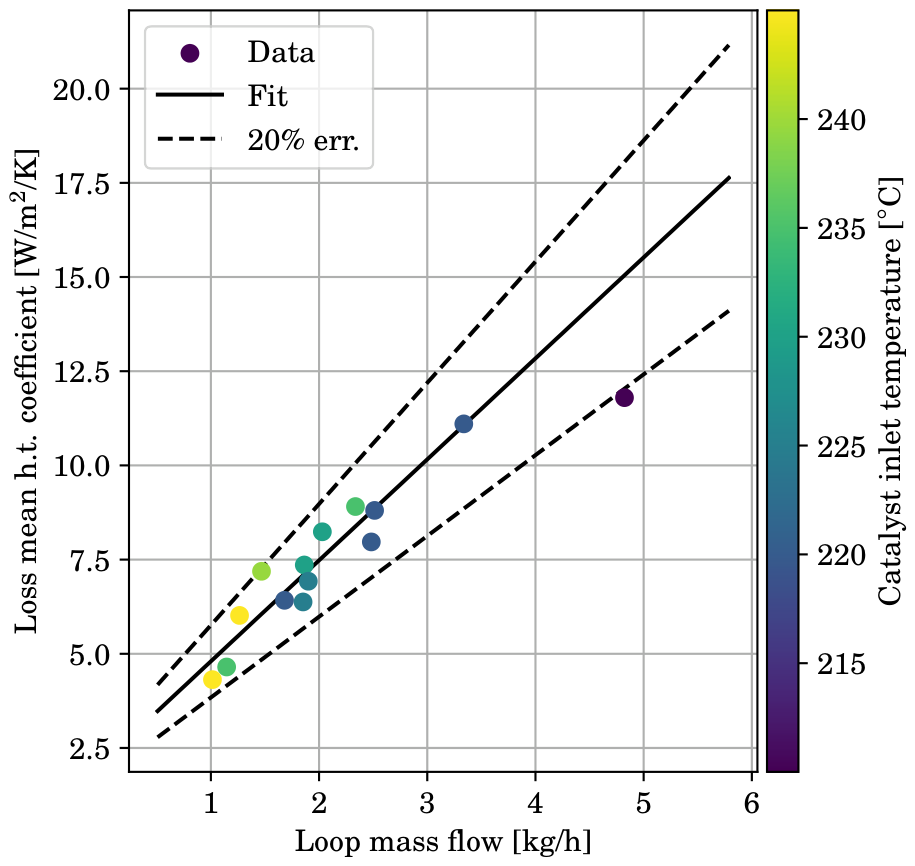
The heat transfer coefficients calculated from all experiments are compared and plotted as a function of the model-predicted mass flow in Figure 4, Figure 5 and Figure 6. Figure 4 shows the catalyst bed to shell heat transfer coefficient as a function of the model-calculated loop mass flow. The data points are slightly scattered, but the general trend shows an increasing heat transfer coefficient with increasing mass flow. This is not remarkable, looking at the similarity of the temperature profile in the reactor between the different experiments (as discussed in van Schagen et al. [31]). The catalyst bed inlet temperature is shown via the color of the data points. This parameter is, however, correlated to some degree with the mass flow as at higher bed inlet temperatures, there is a higher single-pass conversion (in the kinetically limited regime, which prevails here) and therefore a lower mass flow. A simple linear correlation for the heat transfer coefficient as a function of the mass flow is fitted to these data for use during the sensitivity analyses. Table 2 shows the fitted parameters. The right-most point (at a mass flow of around 4.8 kg h−1) is considered an outlier (since steady state was not achieved during this experiment) and not taken into account when fitting a correlation. The correlation can describe the data (except the outlier) with an error of 20% or less. It must be noted here that this correlation is specific to the setup used in this paper and cannot reliably be extrapolated to other systems with different dimensions or a different configuration.
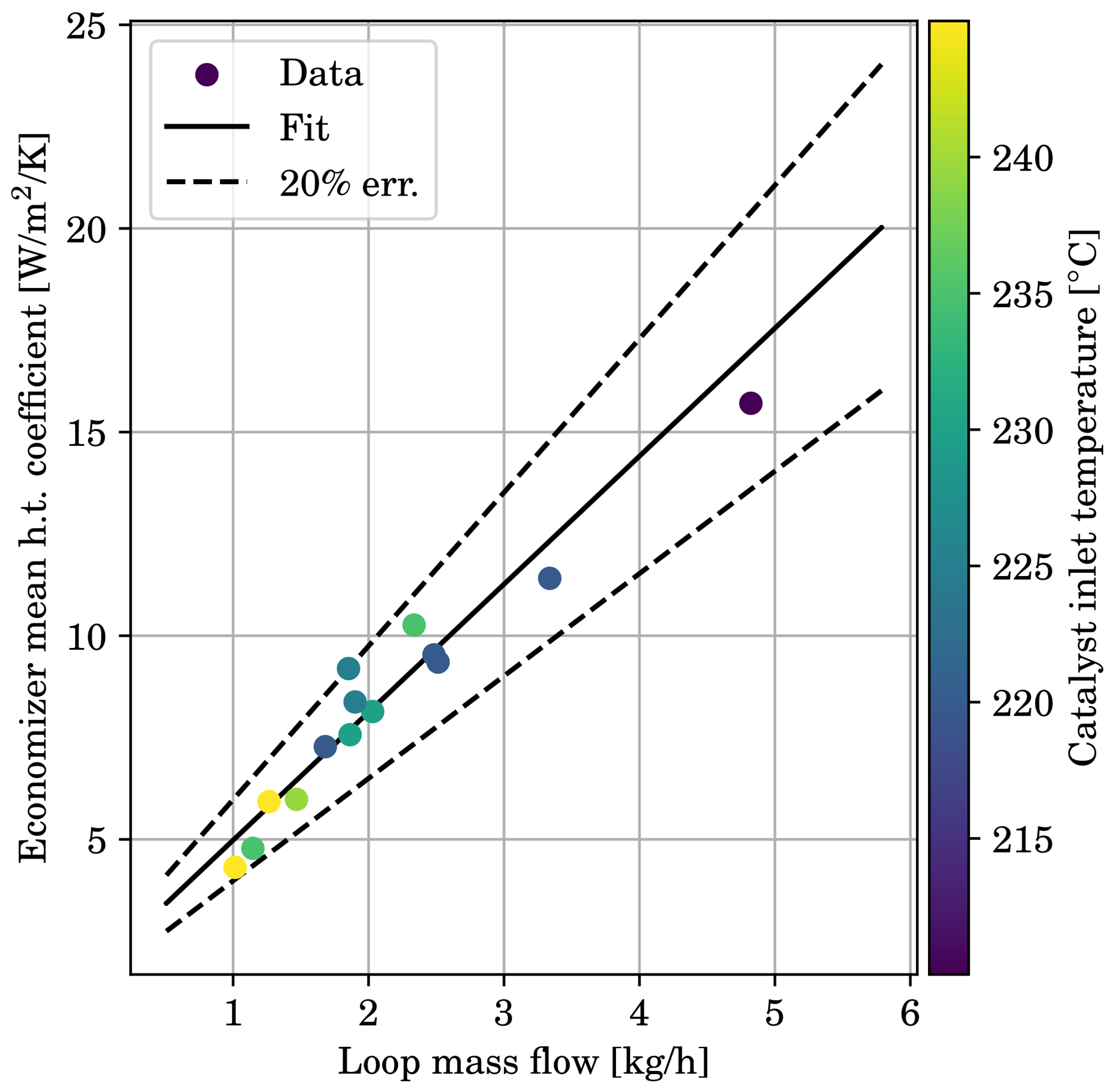
Similar observations are made on Figure 5 and Figure 6, which show the mean apparent heat transfer coefficients for heat integration and heat losses to the environment in the tube-and-shell economizer zone of the reactor. The general trends in both figures are equal: with an increasing mass flow, the apparent heat transfer coefficient increases. Again, this is expected based on the similar temperature profiles measured in the different experiments (see van Schagen et al. [31]). For both mean heat transfer coefficients, a linear correlation for the coefficient as a function of the mass flow is fitted for use during the sensitivity analyses. Table 2 shows the fitted parameters. Both the economizer heat transfer coefficient and the heat loss coefficient are reasonably well described by the correlations; the data are described with an error of 20% or less. It is emphasized again that these correlations are specific to the setup and cannot be reliably extrapolated to other systems.
In general, the apparent heat transfer coefficients (especially in the economizer section) are low—lower even than for laminar pipe flow. This effect is attributed to the local natural convection phenomena, which cause internal circulations in the tube and shell sides. This, in turn, causes the actual driving force for heat transfer to be lower than the one calculated based on the mean temperatures in the tube and shell sides. An extended, a more detailed description for the heat transfer in the reactor is therefore desired to make the model results more accurate and predictable.

3.2. Experimental Comparison

Many variables like temperature, pressure and composition can be measured in the experimental setup. The internal circulation flow, single-pass conversion and energy balance, however, cannot be easily measured experimentally. The model is therefore used to predict these variables for the various experiments. Figure 7 shows the model-calculated single-pass carbon conversion for the various experiments at high, varying pressure and varying catalyst bed inlet temperature. Looking at the trend with pressure, we can see that initially, the conversion rises with pressure to a maximum and then slowly decreases again. This is the effect of two opposing phenomena: the kinetics become faster with pressure, but the recycle flow also becomes higher (see Figure 8, showing the calculated recycle flow for the different conditions), which shortens the residence time. Initially, the former effect is stronger, leading to the increase in single-pass conversion. At higher pressure, the effect of the increasing natural convection starts to dominate (as evidenced by Figure 8), causing the conversion to decrease again—albeit only slightly. This is supported by the experimental data of van Schagen et al. [31], where it was found that the productivity increases significantly with pressure.
A more simple trend is visible in Figure 7 when looking at the effect of catalyst bed inlet temperature on the single-pass conversion. When this temperature rises, the kinetics become faster, leading to a higher single-pass conversion. This indicates that at the current conditions, the reactor is most probably operating in the kinetically-limited regime, as in the equilibrium-limited regime, an opposite effect is expected. Looking at Figure 8, it is clear that for most experiments, the effect of the catalyst bed inlet temperature on the recycle flow rate is minor with the exception of the experiment at 80 bar and a catalyst inlet temperature of 210 °C. At this temperature, the reaction kinetics in the model become slow, so that a relatively large recycle is required to achieve the experimentally measured conversion. It is probable that for this experiment, the model-predicted mean catalyst bed temperature is too low, leading to a too-high recycle flow prediction.
When comparing the model-predicted mass flow in Figure 8 (points, left y-axis) to the trend in anemometer output in the same figure (error bars, right y-axis), there are large differences. The effect of pressure on the anemometer output is minor, while there is a pronounced effect on model-predicted mass flow. Also, the anemometer output is significantly influenced by the catalyst bed inlet temperature, while the model-predicted mass flow is affected much less. One possible cause for the discrepancy between these results is a radial temperature gradient in the catalyst bed. In the model, the bed is modeled in 1D, neglecting all radial temperature gradients. Since heat transfer from the bed to the shell side is significant, however, it is possible that radial temperature gradients exist in the bed, which affect the reaction rate. Therefore, the model might overpredict the conversion, especially for the experiments with a high bed inlet temperature, causing it to predict a too-low recycle flow rate. A 2D reactor model of the catalyst bed section was developed to further investigate this.
Details about the 2D model are discussed in Section S12 of the Supplementary Information, but an example of the results is shown here. Figure 9 shows the mixing-cup-averaged axial temperature profiles calculated by the 1D model and the 2D model. For the 2D model, two situations are investigated: one where the heat transfer resistance lies fully on the shell side (‘shell lim.’) and one where the heat transfer resistance lies fully inside the catalyst bed (‘bed lim.’). For details, the reader is referred to the Supplementary Information. The shaded areas in Figure 9 show the temperature range encountered in the 2D model results. The 1D trend and the 2D trend with the heat transfer resistance on the shell side are very similar in shape, but the temperature predicted by the 2D model is higher. This leads to a higher reaction rate and subsequently a higher single-pass conversion (11.9% in the 1D model, 14.2% in the 2D model). This difference in conversion is significant and will lead to different results for especially the recycle flow if the 2D reactor model is used in the flowsheet calculations. There is a large difference between the 1D trend and the 2D trend with the heat transfer resistance in the bed. The temperature drops quickly from the inlet of the bed due to the rapid heat transfer to the shell side. This causes the reaction to slow down, leading to a low single-pass conversion (only 5.6%). Thus, depending on where the resistance for heat transfer from the catalyst bed lies, the 2D model predicts either a higher or much lower conversion than the 1D model. It must be noted, however, that the results in the case where the heat transfer resistance is located at the shell side are likely more realistic, as the thermal conductivity of the bed is relatively high. Furthermore, CFD simulations (conducted as part of the project but not discussed in this paper) also suggest that the heat transfer resistance in the catalyst bed section of the reactor lies mainly at the shell side. A more detailed investigation of the heat transfer phenomena around the catalyst bed is recommended to clarify the matter in future work.
Figure 9. Mixing-cup averaged axial temperature profiles calculated from the 1D model, the 2D model with the heat transfer resistance at the shell side, and the 2D model with the heat transfer resistance in the bed. The shaded areas show the temperature range in the 2D results.
Chemengineering 10 00062 g009
Another possible cause for the overprediction of the conversion is a measurement error in the catalyst bed inlet temperature. The thermocouple located just before the catalyst bed is also located close to the bed preheater. Since the preheater temperature is high during the reactor operation (due to poor heat transfer from the heater surface to the gas phase), it is very possible that the thermocouple measures a higher temperature than the average gas temperature entering the catalyst bed. This will also lead to a lower conversion. Improving the heat transfer around the heater in the experimental setup and a different placement of this thermocouple can solve this issue. Furthermore, the bed inlet temperature is only measured in the central tube of the multitubular reactor. It is possible that the temperature in the outer tubes (where it is not measured) is lower than in the central tube (due to, for example, heat losses to the environment), causing the mean bed inlet temperature to be lower than the measured value. The addition of thermocouples in the outer tubes is therefore recommended for future work.
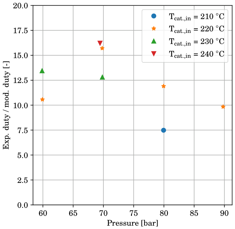
To further analyze the possible overprediction of the conversion by the model, the ratio of the experimentally measured catalyst preheater and condenser duty to the model-calculated values is investigated. The idea is as follows: if the experimentally measured duties of the catalyst bed preheater and condenser are both much higher than the model-predicted values, it is likely that the model predicts a too-low recycle flow rate (and thus a too-high single-pass conversion). Figure 10 and Figure 11 show remarkably similar trends in the duty ratios for the catalyst preheater and condenser. Comparing these results with Figure 8 (showing the model-predicted mass flow) shows that the duty ratio is largest for the points with the smallest predicted mass flow and vice versa. This indicates that the mass flow predicted by the model is probably too low for all experiments and also that the recycle mass flow is probably much more similar in all experiments than the model predicts. The absolute value of the trends in Figure 10 and Figure 11 is likely a coincidence, as there are undesired heat transfer mechanisms both at the preheater and condenser. At the preheater, heat is lost to the reactor flange due to conduction in the heater, while at the condenser, the electrical tracing present there increases the condenser duty. If these heat sidestreams are known (they can be determined, for example, from a series of experiments under inert conditions at different flow rates), the condenser duty and preheater duty can be used to estimate the recycle flow. It is recommended to investigate this possibility further with future experiments.
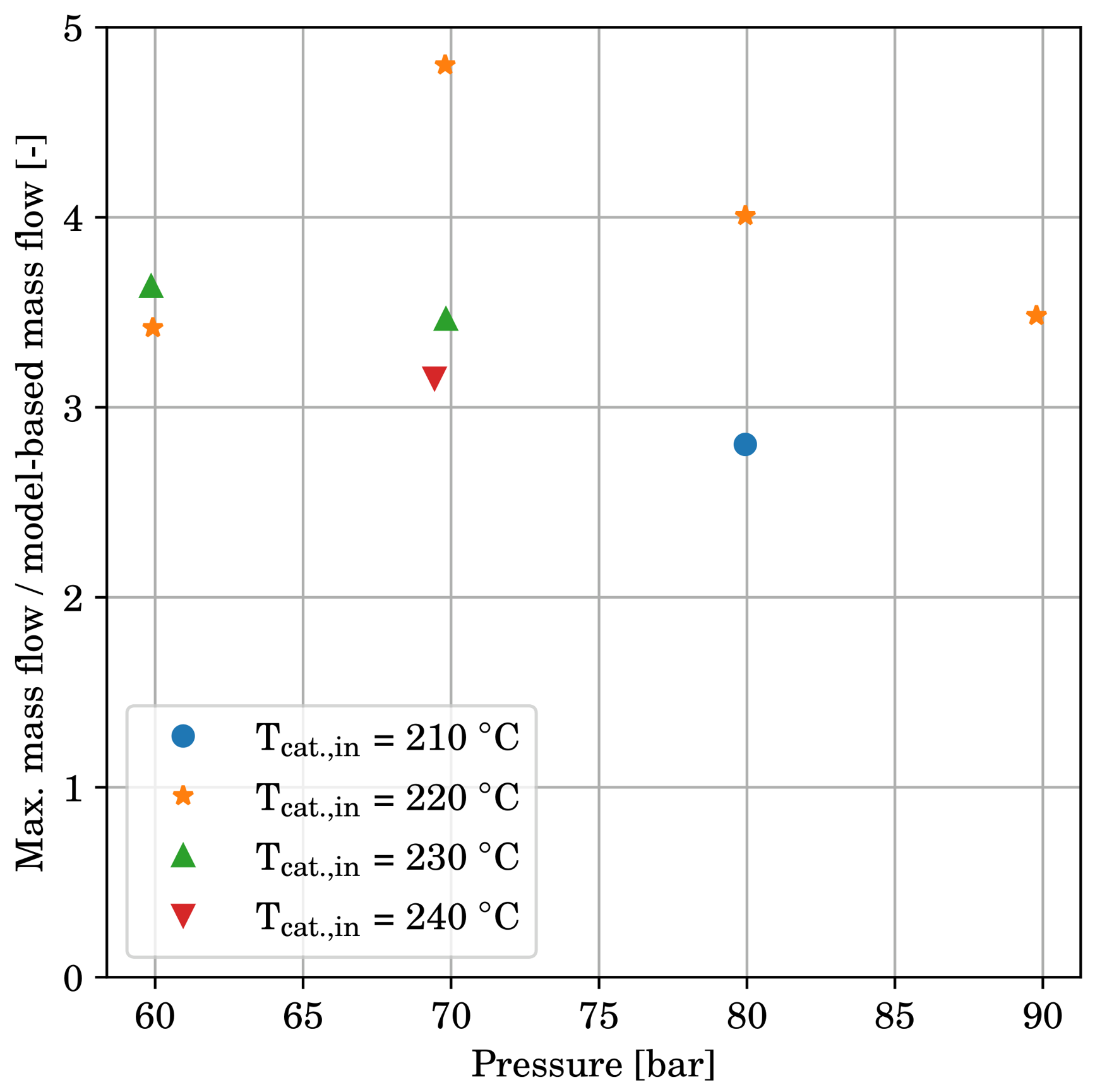
To further investigate if the hypothesis of an underprediction of the loop mass flow by the model is plausible, Equation (7) is used to calculate the maximum possible loop mass flow in the reactor for all experiments. This value is then divided by the model-calculated flow and plotted in Figure 12. In this figure, more or less the same trend is visible as in Figure 10 and Figure 11. Furthermore, the values of the maximum and model-calculated mass flow are in the range of 2.8 to 4.8, confirming that indeed, a higher mass flow can exist in the reactor than the model currently predicts.
In summary, Figure 8 and Figure 10, Figure 11 and Figure 12 indicate that the model-predicted single-pass conversion and consequently the predicted recycle mass flows are very sensitive to the temperature in the catalyst bed. The experimentally measured duties of the catalyst bed preheater and condenser are much larger than the model-predicted ones, hinting that the recycle flow in the setup might be higher than the model predicts. This hypothesis is supported by the fact that the maximum natural-convection driven mass flow calculated by Equation (7) is 2.8 to 4.8-fold larger than the model-predicted mass flow. This effect could be caused by radial temperature gradients in the catalyst bed that are currently not taken into account in the full reactor model. A study with a separate 2D model of the catalyst bed confirms that radial gradients in the bed may indeed have a significant effect on the single-pass conversion predicted by the model, and this effect should be further investigated in future experimental and modeling work. A permanent inclusion of the 2D catalyst bed model in the full reactor model is recommended for future work albeit at significant extra computational effort. A measurement error in the bed inlet temperature is another possible cause of the deviations in mass flow.
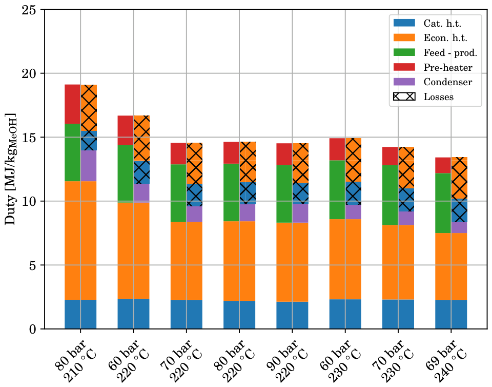
Finally, the model is used to calculate the energy flows in the setup. Figure 13 shows the energy balance over the reactor as calculated by the model for the experiments at varying pressure and catalyst bed inlet temperature. For each experiment, two bars are shown: the left bar shows the energy input streams and the right bar shows the energy output streams. Since a steady-state situation is assumed, there is no accumulation of heat, and therefore, the two bars are of equal size for each set of conditions. The bottom two sections of the bar correspond to heat integration at the catalyst bed and the economizer section (e.g., the amount of heat transferred from the catalyst bed to the shell (blue) and from the economizer tube side to the shell (orange)). Since these are internal heat streams, they are of equal size in the left and right bars. The green part of the left bars shows the difference in enthalpy flow between the feed and product streams of the reactor (most significantly influenced by the reaction heat and to smaller extent by the feed temperature). The red part of the left bar corresponds to the preheater duty and the purple part to the heat withdrawal in the condenser. Finally, the hatched parts of the right bar correspond to heat losses to the environment in the shell around the catalyst bed (blue hatched part) and the shell side of the economizer section (orange part).
From Figure 13, it becomes clear that for all conditions, the largest amount of heat integration takes place in the economizer section, as is expected. However, significant heat integration also happens at the catalyst bed despite it being only a small section compared to the rest of the reactor. The significant amount of heat transfer happening here also strengthens the suspicion of significant radial temperature gradients in the bed itself. When looking at the top part of the bars, it is clear that for all experiments, the apparent heat losses (hatched parts) are larger than the preheater duty. If the heat losses are reduced (for example with better insulation), the hatched area would be reduced in size. Since both bars must be of equal size, the left bar must therefore also be reduced in size—for instance, by lowering the preheater duty (red part, potentially to zero) or lowering the feed temperature (green part). This means that if the heat losses were minimized, the reactor can operate autothermally. It must be noted, however, that the model probably underpredicts the recycle ratio, and that at a higher recycle ratio, the picture will change. Most notably, the condenser duty will increase (because of the larger amount of sensible heat that is removed at higher recycle ratios), and therefore, the window for autothermal operation becomes more narrow.
Overall, the model gives some useful insights in the experimental data mainly with regard to energy flows, heat transfer and recycle mass flows. It is, however, likely that the model overestimates the single-pass conversion in the catalyst bed. A possible cause for this is the effect of radial temperature gradients in the bed, which is presently not included in the flowsheet model; inaccurate (too low) experimental measurements of the inlet temperature are another possible cause. According to the model results, sufficient heat integration takes place to operate autothermally if the heat losses to the environment are mitigated. The majority of the heat integration takes place in the economizer section, but a sizeable amount of heat transfer also takes place around the catalyst bed, indicating that radial temperature gradients there may indeed be significant.

3.3. Natural Convection

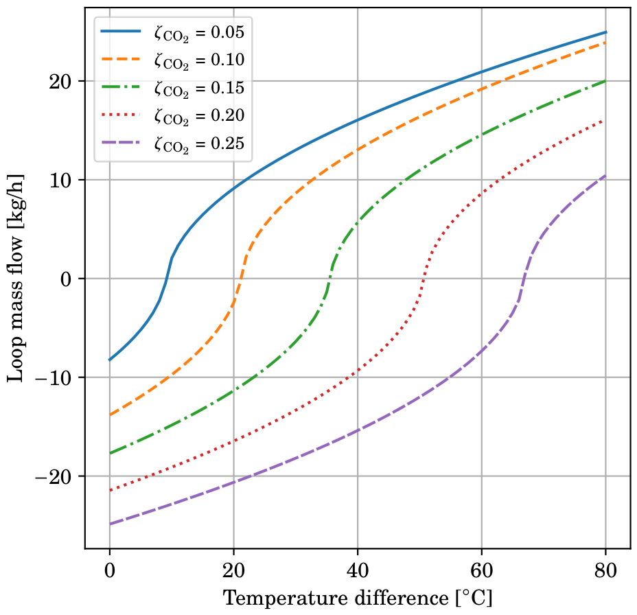
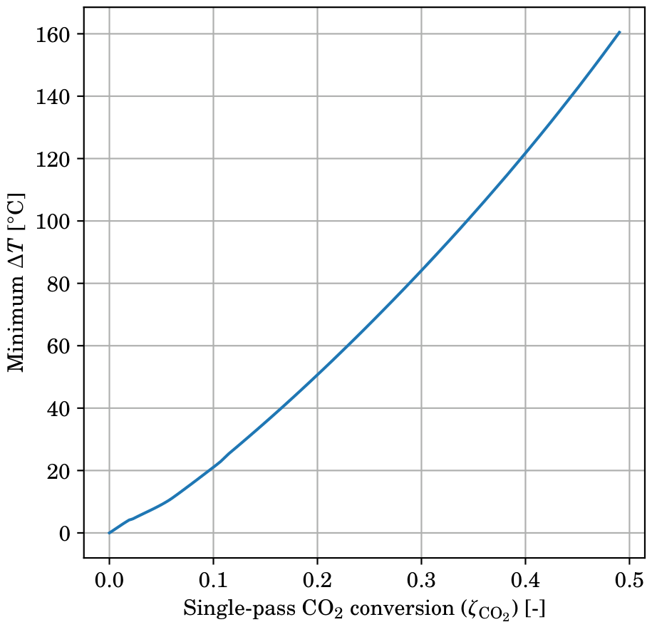
The previous section shows that the recycle flow in the reactor is an important parameter in the model. The effects of the temperature difference between the tube and shell sides of the reactor and the single-pass conversion on the achievable recycle flow are therefore further investigated. Because the mean molar mass of the gas in the shell side of the reactor is lower than that in the tube side of the reactor (since the relatively heavy methanol and water are removed in the condenser), at the same temperature, the density of the tube-side gas is higher than that of the shell-side gas. This would lead to a reverse flow in the reactor. To achieve flow in the correct direction, there is a minimum temperature difference required between the two sides so that the gas density in the shell side becomes higher than in the tube side. Figure 14 shows this minimum temperature difference (at a catalyst bed temperature of 220 °C and 80 bar with an isothermal catalyst bed) as a function of the single-pass conversion. At higher conversions, a higher temperature difference is required, which is expected, as the rising conversion increases the composition difference between the tube and shell sides of the reactor. At high conversions (above 30%), the minimum temperature difference becomes very large (even above 100 °C), making it difficult to achieve flow in the correct direction under these conditions. In practice, however, such conversions are hard to achieve in the setup because of kinetic or equilibrium limitations. Still, if there is too much heat integration or too much heat loss to the environment, it is a challenge to generate sufficient natural convection flow.
In addition to the minimum temperature difference for natural convection, the maximum flow that can be generated at a certain temperature difference is also of interest. This is shown in Figure 15 where the maximum recycle flow (calculated with Equation (7)) is plotted as a function of the temperature difference and the single-pass conversion (again assuming an isothermal catalyst bed with a temperature of 220 °C and at 80 bar). Below the minimum temperature difference, the calculated mass flow is indeed negative (e.g., in the wrong direction), which is obviously undesired. Just above the minimum value, the achievable mass flow steeply increases with the temperature difference. This is mainly because of the quadratic dependency of the friction force on the velocity (see Equation (7)). After this, the achievable mass flow rises more slowly but keeps increasing with the temperature difference. At a certain temperature difference (i.e., 50 °C), the single-pass conversion has a profound effect on the achievable mass flow. At conversions higher than 20%, the mass flow is in the wrong direction. However, at 15% conversion, a mass flow of above 10 kg h−1 is already achievable. If the temperature difference in the reactor is small (which it is—the experimentally measured temperature difference is in the order of 50 °C, see van Schagen et al. [31]), the mass flow and thus the reactor performance are largely affected by the single-pass conversion. If the temperature difference becomes too small, reverse-flow oscillations may occur in the reactor, and while the system is able to stabilize itself, these oscillations negatively affect the productivity. It is therefore important to minimize heat losses from the tube side to the environment and optimize the heat integration in the reactor.

3.4. Sensitivity Analyses

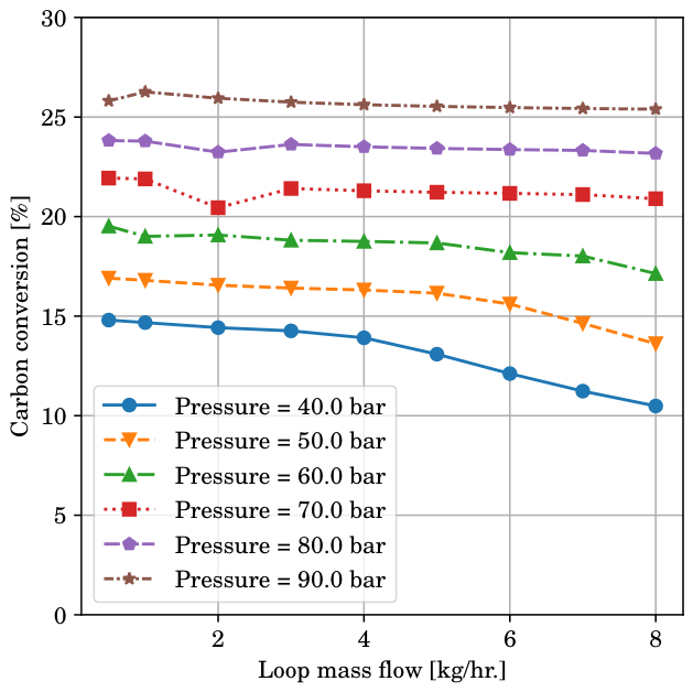
To explore the effect of the operating conditions on the reactor performance, sensitivity analyses on several operating parameters are performed using the model. Because of the steady-state 1D nature of the model and the optimized thermodynamics engine, the model is reasonably fast (one data point is calculated in around five seconds; for more details, see Section S10 in the Supplementary Information), meaning that sensitivity can be achieved in an acceptable amount of time. During these sensitivity analyses, heat losses are neglected, because it is expected that when scaling up the setup, heat losses are less important than in the current pilot setup (due to the reduced surface-to-volume ratio and because better insulation can be applied). It should, however, be taken into account when looking at the results that they represent an optimal case without heat losses, and that due to heat losses, some parameters (like carbon conversion) might be slightly lower in reality. Figure 16 shows the effect of the pressure and recycle mass flow on the single-pass conversion. At a given pressure, the carbon conversion tends to decrease with the mass flow. This is expected, and it is caused by a decreasing residence time when the loop mass flow increases. The productivity, however, always increases with increasing recycle flow (as the productivity is the product of the flow and conversion). If the single-pass conversion becomes too low, however, autothermal operation becomes unfeasible, which limits the operating range of the reactor (see Section 3.5). Also, very high mass flows are not achievable by natural convection, which is an effect which is not taken into account in Figure 16. The optimal mass flow is therefore the highest flow where autothermal operation and natural convection-driven flow are still achievable. At a constant mass flow, there is a clear positive effect of pressure, which is caused by the faster kinetics and more favorable equilibrium at higher pressure. This once again emphasizes the advantage of operating at high pressure.
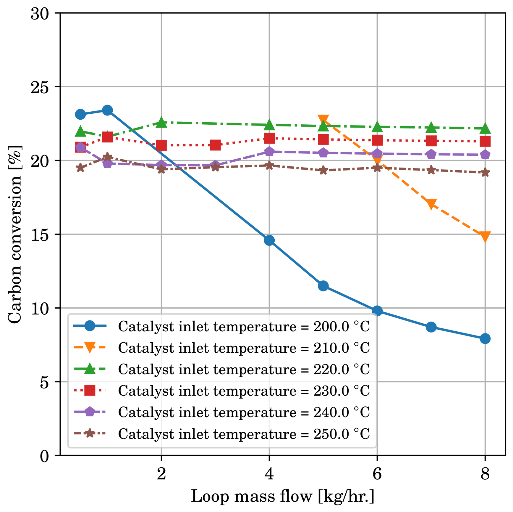
Figure 17 shows the effect of the catalyst bed inlet temperature and recycle mass flow on the single-pass conversion. At low mass flows, the conversion is high, because equilibrium is always reached in the catalyst bed. This also means that at low mass flow, if the bed inlet temperature decreases, the conversion increases as the equilibrium conversion decreases with temperature. For the lower bed inlet temperatures, at some point, the conversion starts to drop with increasing mass flow. At this point, the kinetics become so slow that equilibrium is no longer reached and kinetic limitations prevail. For higher bed inlet temperatures, this does not happen (at the mass flow range displayed) because of the faster kinetics at a higher temperature. It is thus favorable to operate at a bed inlet temperature high enough to just approach equilibrium but not so high that the conversion starts to decrease again. In this way, optimal utilization of the catalyst bed in ensured.
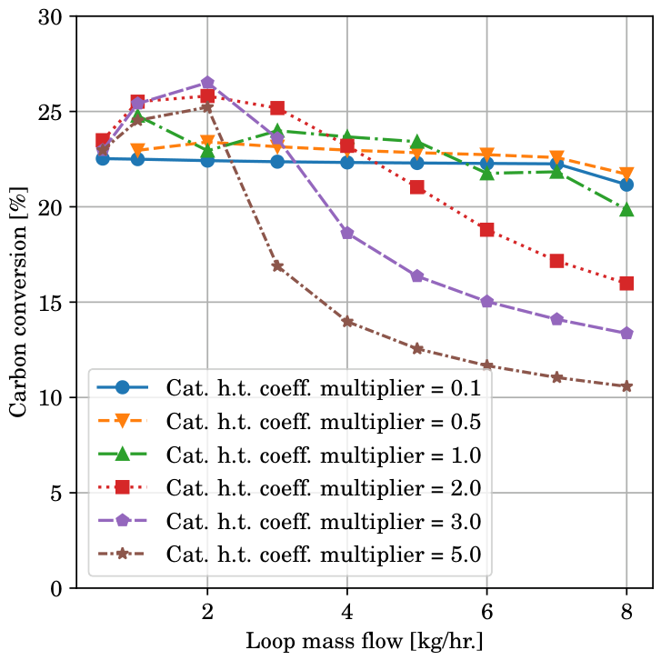
Another important parameter is the heat transfer coefficient in the catalyst bed (which is not easily measured). This parameter was therefore varied by multiplying the coefficient calculated with the shortcut correlation (Table 2) with a certain factor. Figure 18 shows the single-pass conversion as a function of the recycle mass flow in the reactor and the catalyst bed heat transfer coefficient factor. At low heat transfer coefficients, the bed operates near adiabatically (the blue line) and equilibrium conversion is achieved. Only at high mass flow rates does the residence time become so short that equilibrium is no longer reached, and the conversion starts to decay. When the heat transfer coefficient starts to increase, the conversion increases as well. This due to the heat transfer from the catalyst bed to the shell, which lowers the outlet temperature of the bed and increases the equilibrium conversion. At very high heat transfer coefficients and sufficiently high mass flows, the conversion rapidly drops because now heat transfer is so fast that the temperature in the bed becomes low enough for the system to become kinetically limited.
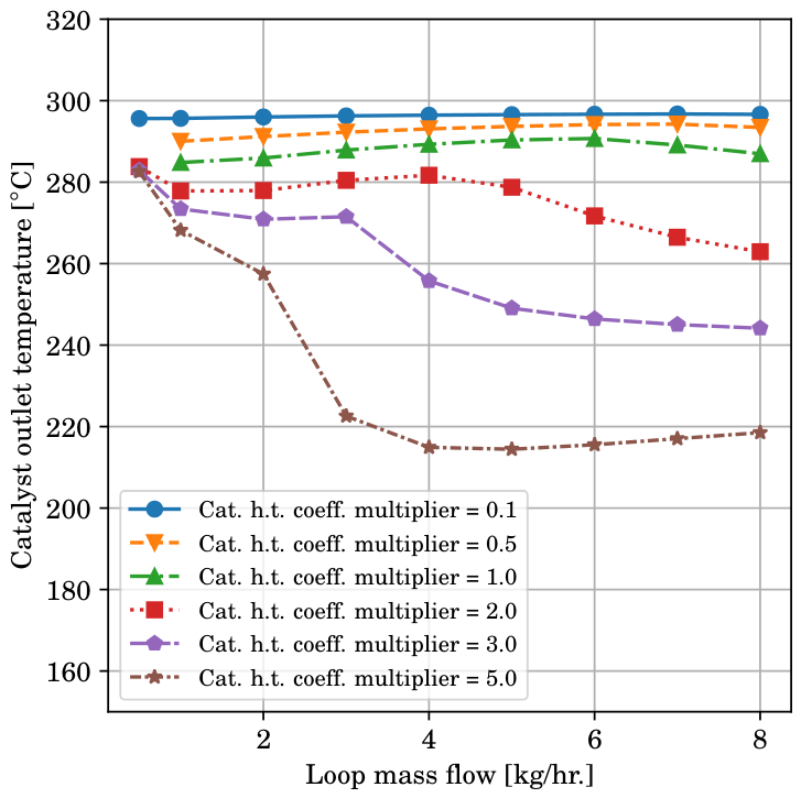
Figure 19 shows the catalyst bed outlet temperature for the same simulations. At low heat transfer coefficients, the outlet temperature approaches the adiabatic outlet temperature. As the heat transfer coefficient increases, the bed outlet temperature becomes lower, as expected. When the heat transfer becomes very fast, the figure confirms that the temperature drops to a low value (the brown line), at which point the reaction kinetics become slow enough for the system to be kinetically limited. The results show that some heat transfer around the catalyst bed is beneficial, as this increases the equilibrium conversion by lowering the bed temperature. Lowering the bed temperature has the additional benefit of better catalyst stability. Too much heat transfer, however, is not favorable, as then the temperature in the bed becomes too low, causing kinetic limitations to limit the conversion and thus the productivity (at a given mass flow).

3.5. Minimum Conversion Required for Autothermal Operation

It is possible to estimate the minimum single-pass conversion that is required to operate autothermally based on a shortcut method. The basis for this method is an energy balance over the entire reactor. If the reactor operates autothermally, the only energy streams in and out of the reactor are the feed flow, product flow and duty of the condenser equated in Equation (9), where h ˙ is an enthalpy flow in W . Working this equation out leads to Equation (10) where H denotes the specific enthalpy in J kg−1, m ˙ a mass flow in kg s−1 and Δ c H the heat of condensation (in J mol−1). A mass balance over the reactor tells us that the outlet mass flow (of liquid from the condenser) has to equal the feed mass flow, which is a fact that has been used in Equation (10). The last parts of the equation account for the sensible and latent heat withdrawn in the condenser. The factor half comes from the product composition. The composition of the inlet and outlet streams is known in the steady state; the feed consists of a 75/25 mol/mol mixture of H2/CO2, while the product consists of a 50/50 mol/mol mixture of methanol/water, allowing the feed and product enthalpies to be calculated. The heat capacity of the gas in the condenser C p can be estimated based on a typical recycle gas composition. The temperature difference over the condenser can similarly be estimated; typically, it is in the range of 60 °C to 100 °C when there is sufficient heat integration in the reactor. Finally, the internal reactor mass flow m ˙ internal is calculated from the single-pass conversion as m ˙ internal = m ˙ ζ . Rearranging yields Equation (11), which allows calculating the minimum single-pass conversion required for autothermal operation when operating with a stoihiometric 1:3 CO2:H2 feed.
0 = h ˙ feed h ˙ product + Q cond .
0 = m ˙ H feed m ˙ H product + m ˙ internal C p Δ T cond . + m ˙ M ¯ w , product 1 2 Δ c H MeOH + Δ c H water
ζ min = C p Δ T cond . H feed H product 1 M ¯ w , product 1 2 Δ c H MeOH + Δ c H water
As an example, assuming a condenser temperature difference of 80 °C, a fresh feed temperature of 200 °C, a product temperature of 60 °C and a pressure of 60 bar leads to a minimum single-pass conversion of 13.8%, which is a realistic value when compared to the values found in the sensitivity analyses later in this section. The equation shows that by lowering the temperature difference over the condenser (by raising the condenser temperature or improving heat integration in the economizer section), a lower single-pass conversion is allowed for autothermal operation. However, care must be taken to keep the condenser temperature low enough so that sufficient methanol and water are condensed. Similarly, increasing the feed temperature also gives a broader range for autothermal operation (by increasing H feed ), which makes sense. The simple equation can be used as a convenient tool to check if a design is feasible when scaling up or optimizing the reactor.

3.6. Operability Range

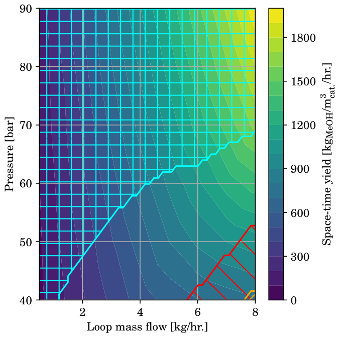
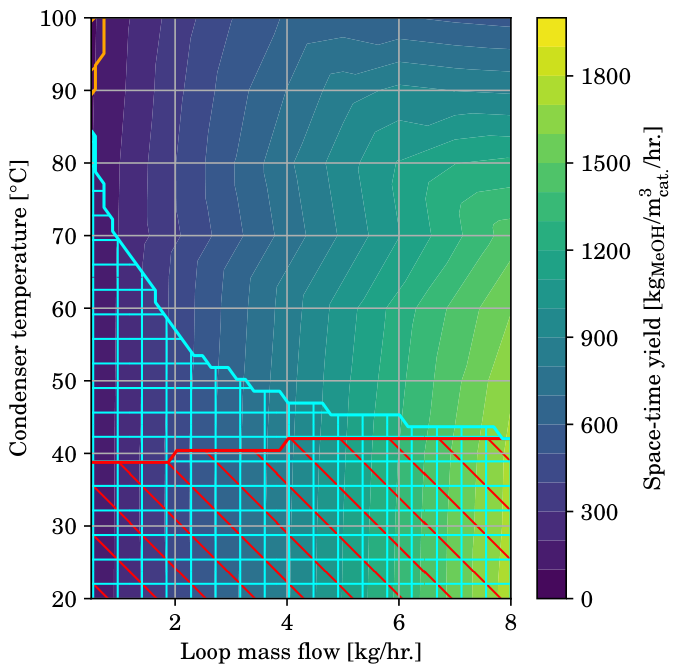
It is important to know in which range of operating conditions it is feasible to operate the reactor autothermally. With this information, the optimal operating conditions can be found. To this end, the sensitivity analyses from the previous section are extended and visualized in an alternative way. All of these simulations are run without taking into account heat losses to the environment (thus assuming a perfectly insulated setup for the same reasons as discussed in Section 3.4). If heat losses would be taken into account, the region of autothermal operation would become slightly smaller. Figure 20 shows the operability range as a function of the pressure and loop mass flow at a catalyst bed inlet temperature of 220 °C and a condenser temperature of 40 °C. The background color shows the space–time yield of the reactor (see also the color bar). Then, there are three types of hatched areas. Inside the cyan hatched area on the left-hand side, condensation will happen inside the tubes of the reactor (because there is too much heat integration). This is undesirable, but it can be solved by hindering the heat transfer in the economizer section (for example, by insulating part of the tubes). Inside the orange-colored area, the natural convection driving force is insufficient to generate the recycle flow, meaning that it is impossible to operate in this area. The red hatched area shows the conditions where autothermal operation is infeasible.
The unhatched area in Figure 20 is relatively narrow, meaning that proper operation is possible only at low pressures but at a wide range of mass flows. However, a large portion of the graph is covered by the blue hatched area, indicating that heat transfer is essentially too fast (leading to premature condensation in the economizer section). The size of this section is, however, largely influenced by the description of the heat transfer coefficients, for which a shortcut description is used in the model. It is therefore likely that the actual feasible operating range is larger than the current unhatched area shown, but further investigations into the heat transfer behavior of the reactor to create more accurate correlations for the heat transfer coefficients is required. There is only a small area in the bottom right of the graph where the natural convection force is insufficient to drive the recycle. Looking at the productivity, there is a clear increasing trend from the bottom-left corner (low pressure and mass flow) to the top-right corner. Overall, the figure shows that autothermal operation is possible at a wide range of conditions (if heat losses are prevented in the setup) and that at higher mass flows, significantly higher productivities can be achieved in the setup—up to more than three times the maximum currently measured productivity.
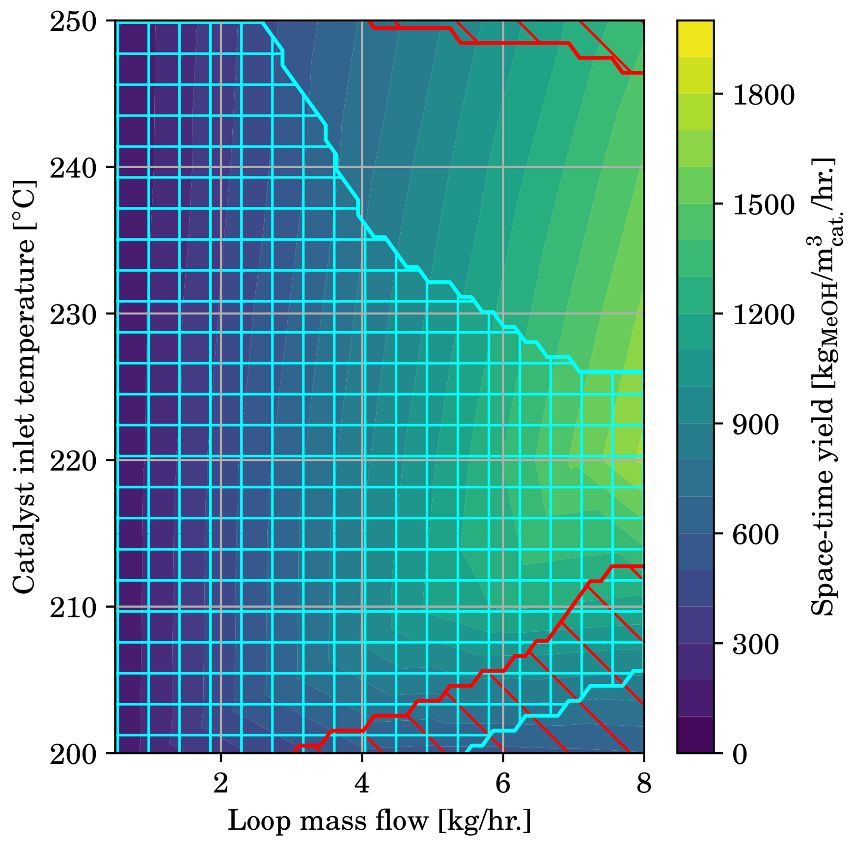
Figure 21 shows the operability range and productivity as a function of the catalyst bed inlet temperature and mass flow. The operability range is narrow in terms of bed inlet temperature but wide in terms of mass flow. At low mass flows, heat transfer is so fast that condensation already starts to happen prematurely at low and high bed inlet temperatures. At too-high mass flows, the single-pass conversion becomes too low, making autothermal operation is infeasible. Again, the cyan area is relatively large, and its position may move toward the left if a better and more favorable description for the heat transfer coefficients is obtained. The productivity has a maximum at high mass flows and a moderate bed inlet temperature due to the trade-off between kinetics and equilibrium. At low bed inlet temperatures, the reaction is kinetically limited so that the conversion increases with temperature. It is therefore most optimal to operate at a bed inlet temperature that yields a near-equilibrium conversion at a mass flow as high as possible where autothermal operation is still possible.
Figure 22 shows the effect of loop mass flow and condenser inlet temperature on the operability range and productivity. When the condenser temperature is low, too much heat is withdrawn in the condenser, making autothermal operation infeasible. This effect increases slightly when the mass flow increases. At low mass flow, a premature condensation of methanol and water starts to happen, leading to non-optimal operation. If the condenser temperature would be increased further (above 100 °C), however, insufficient condensation of methanol and water would take place, leading to a significant methanol and water recycle, thereby lowering the single-pass conversion and rendering autothermal operation impossible. Also, from a productivity perspective, it is best to operate with a low (but not too low) condenser temperature of around 40 °C to 50 °C.
From Figure 20, Figure 21 and Figure 22, it is concluded that with the current heat transfer description and no heat losses to the environment, autothermal operation is possible at a reasonable range of conditions. At a wide range of conditions, internal heat transfer is essentially too fast, leading to methanol and water condensation in the tubes, which should be avoided. The heat transfer correlations used in the model are, however, calculated with a shortcut method from a limited set of experimental data, leading to some uncertainties. If the heat transfer in the economizer section would be better than predicted by the correlation, the area where autothermal operation is possible would increase in size, but so will the area in which premature condensation takes place, and vice versa. Then, the heat transfer from the catalyst bed will affect mainly the conversion and catalyst bed outlet temperature (see also Figure 18) and thereby the area where autothermal operation is possible. In the kinetically-limited regime (at relatively high mass flows and low catalyst bed inlet temperatures), the operability range will increase with a decreasing heat transfer coefficient. In the equilibrium-limited regime, the effect is exactly opposite. In terms of pressure, catalyst bed inlet temperature and condenser temperature, autothermal operation is possible at a wide range of conditions. Maximum productivity (up to 2000 kg MeOH m cat . 3 h 1 ) with autothermal operation is predicted at high pressure (as high as possible), a medium catalyst bed inlet temperature (around 220 °C) and a low condenser temperature (40 °C), neglecting any heat losses to the environment.


3.7. A Perspective on Scaling Up

Ultimately, it is desirable to scale up the system studied in this paper to a commercial scale, for which the model developed here can be a useful tool. This paragraph briefly discusses the perspective on scaling up the present system. Obviously, when scaling up, it is desirable to maintain the favorable characteristics of the design (e.g., the natural-convection driven flow and the autothermal operation). Since the operability window not only depends on the operating conditions but also on the design, care must be taken to carefully scale up the system. In the present design, the length of the catalyst bed is limited by the maximum pressure drop that can be overcome by free convection (see also Equation (7)). Thus, if the length of the catalyst bed is increased in a scaled-up design, the driving force for natural convection must also be increased, for example, by increasing the total height of the system. If the total height is increased while keeping the tube diameter constant, however, there would be too much area for heat transfer. Therefore, the tube diameter should therefore be increased as well (to reduce the heat transfer coefficient at constant Nusselt number) or an insulated tube section should be added. Ultimately, the most straightforward manner of scaling up the current system is to increase the shell diameter and add more tubes. A lower surface-to-volume ratio will decrease heat losses (which is favorable), and the maximum production rate is expected to scale linearly with the number of tubes. Since in this case the tube diameters, length and catalyst bed length remain the same, no significant extrapolation of the current experimental results by the model is required.

4. Conclusions

In this paper, a steady-state flowsheet model of a highly integrated, natural convection-driven condensing methanol reactor was successfully implemented. Experimental data were used to validate the model and fit shortcut correlations for the apparent heat transfer coefficients in the model. The model shows that for all experiments, the majority of the heat integration takes place in the economizer section, but significant heat exchange also happens from the catalyst bed to the shell side. If heat losses would be mitigated, the setup is able to operate autothermally in all analyzed experiments. The comparison of the model to the experimental data indicates that the model overpredicts the single-pass conversion (and consequently underpredicts the recycle flow). A factor that could contribute to this is the heat transfer from the catalyst bed to the shell side, which can induce radial temperature gradients, which are presently not taken into account in the flowsheet model. A separate 2D model indicates that such gradients may indeed be significant, and it is recommended to add a 2D catalyst bed model to the full flowsheet model. A systematic measurement error in the bed inlet temperature (so that the actual gas temperature is lower than measured) can also explain the overprediction of the conversion by the model. Model results show that given a single-pass conversion in the catalyst bed, a minimum temperature difference is required for the natural convection flow to be in the right direction. Calculations of the maximum achievable natural convection flow show that this flow has a strong negative correlation with the single-pass conversion and a positive correlation with the temperature difference between the tube and shell sides of the reactor. It is recommended to extend the flowsheet model with a better description for the heat transfer coefficient to improve the accuracy of the model predictions. Sensitivity analyses are conducte with the model while neglecting any heat losses. Their results show that with the present description for the heat transfer coefficient, autothermal operation is feasible at a reasonable range of conditions (in terms of pressure, catalyst bed inlet temperature and condenser temperature). Heat transfer at low mass flows is, however, too fast, leading to premature condensation in the economizer section. If heat transfer at low mass flows is less than currently predicted, the feasible operating range greatly extends and maximum productivity with autothermal operation (up to 2000 kg MeOH m cat . 3 h 1 ) is predicted at high pressure, a catalyst bed inlet temperature of around 220 °C and a condenser temperature of 40 °C.

Supplementary Materials

The following supporting information can be downloaded at https://www.mdpi.com/article/10.3390/chemengineering10050062/s1, Figure S1: Model-calculated dew- and bubble point curves of a methanol-water mixture at different temperatures compared to experimental data from Ghmeling et al.; Figure S2: Model-calculated dew- and bubble point pressures of mixtures of methanol with hydrogen, nitrogen and carbon monoxide compared to experimental data from Brunner et al.; Figure S3: Model CO2 conversion and methanol selectivity as a function of temperature compared to experimental data from Slotboom et al.; Figure S4: Left: Particle friction factor as a function of the modified Reynolds number, experimental data denoted by the points, original Stokes-Ergun equation shown by the blue solid line and the refitted equation shown by the dashed orange line. Right: Parity plot of the experimentally measured and calculated pressure drop over the catalyst bed. The pressure drop is calculated using the refitted Stokes-Ergun equation; Figure S5: Schematic view of the numerical grid for the semi-discretization of the 2D transport equations; Figure S6: Mixing point in a loop; Figure S7: Mixing-point residual over tolerance as function of the number of solution iterations for a typical run of the model in this work; Figure S8: Mixing-cup averaged axial mole flux profiles calculated from the 1D model, the 2D model with the heat transfer resistance at the shell side and the 2D model with the heat transfer resistance in the bed; Figure S9: Temperature profile calculated from the 2D model with the heat transfer resistance at the shell side; Figure S10: Temperature profile calculated from the 2D model with the heat transfer resistance in the bed.; Table S1: Diffusion volumes of the components included in the model. References [54,55,56,57,58,59,60,61,62,63,64,65,66,67,68,69,70,71,72,73,74] are cited in the supplementary materials.

Author Contributions

Conceptualization, T.v.S. and W.B.; methodology, T.v.S. and W.B.; software, T.v.S.; validation, T.v.S. and W.B.; formal analysis, T.v.S.; investigation, T.v.S.; resources, W.B.; data curation, T.v.S.; writing—original draft preparation, T.v.S.; writing—review and editing, W.B.; visualization, T.v.S.; supervision, W.B.; project administration, W.B.; funding acquisition, W.B. All authors have read and agreed to the published version of the manuscript.

Funding

This research was funded by Rijksdienst voor Ondernemend Nederland (RVO) in a Joint Industry Project with No. TEEI119005.

Data Availability Statement

The datasets presented in this article are not readily available because the models developed in this paper are part of an ongoing study. The experimental data used in this paper can be found in the work of van Schagen et al. [31]. Requests to access the datasets should be directed to T.v.S.

Acknowledgments

The authors are grateful to the project partners (Shell, DMT Environmental Technologies, Brusche Process Technology and ISPT) for the support and the useful discussions.

Conflicts of Interest

The authors declare no conflicts of interest.

List of Symbols

SymbolUnitDescription
am2 m−3Specific surface area
A cs m2Cross-sectional area
C p J kg−1 K−1Heat capacity at constant pressure
d p mParticle diameter
DmPipe diameter
f-Friction factor
gm s−2Gravitational acceleration
h ˙ WEnthalpy flow
HmHeight
HJ kg−1Specific enthalpy
LmLength
m ˙ kg s−1Mass flow
M w kg mol−1Molar mass
pPaPressure
QWHeat duty
rmRadius
TKTemperature
um s−1Velocity
UW m−2 K−1Heat transfer coefficient
zmAxial coordinate
ε -Bed void fraction
ζ -Single-pass conversion
ρ kg m−3Density
τ PaShear stress
φ radAngle

References

  1. Olah, G.A.; Goeppert, A.; Surya Prakash, G.K. Beyond Oil and Gas: The Methanol Economy, 2nd ed.; Wiley-VCH John Wiley Distributor: Los Angeles, CA, USA, 2009. [Google Scholar]
  2. Schlögl, R. (Ed.) Chemical Energy Storage; De Gruyter: Berlin, Germany; Boston, MA, USA, 2013. [Google Scholar]
  3. Bertau, M.; Offermanns, H.; Plass, L.; Schmidt, F.; Wernicke, H.J. (Eds.) Methanol: The Basic Chemical and Energy Feedstock of the Future; Springer: Berlin/Heidelberg, Germany, 2014. [Google Scholar] [CrossRef]
  4. Pontzen, F.; Liebner, W.; Gronemann, V.; Rothaemel, M.; Ahlers, B. CO2-based methanol and DME-Efficient technologies for industrial scale production. Catal. Today 2011, 171, 242–250. [Google Scholar] [CrossRef]
  5. Yarulina, I.; Chowdhury, A.D.; Meirer, F.; Weckhuysen, B.M.; Gascon, J. Recent trends and fundamental insights in the methanol-to-hydrocarbons process. Nat. Catal. 2018, 1, 398–411. [Google Scholar] [CrossRef]
  6. Araya, S.S.; Liso, V.; Cui, X.; Li, N.; Zhu, J.; Sahlin, S.L.; Jensen, S.H.; Nielsen, M.P.; Kær, S.K. A review of the methanol economy: The fuel cell route. Energies 2020, 13, 596. [Google Scholar] [CrossRef]
  7. Ministerie van Klimaat en Groene Groei. Verdiepingsdocument Beoordeling Waterstofdragers; Ministerie van Klimaat en Groene Groei: Den Haag, The Netherlands, 2024; pp. 1–40.
  8. Ott, J.; Gronemann, V.; Pontzen, F.; Fiedler, E.; Grossmann, G.; Kersebohm, D.B.; Weiss, G.; Witte, C. Methanol. In Ullmann’s Encyclopedia of Industrial Chemistry; Wiley: Hoboken, NJ, USA, 2012. [Google Scholar] [CrossRef]
  9. English, A.; Brown E&C, J.; Rovner, J.; Davies, S. Methanol. In Kirk-Othmer Encyclopedia of Chemical Technology; Wiley: Hoboken, NJ, USA, 2015; pp. 1–19. [Google Scholar] [CrossRef]
  10. Bowker, M. Methanol Synthesis from CO2 Hydrogenation. ChemCatChem 2019, 11, 4238–4246. [Google Scholar] [CrossRef]
  11. Darji, H.R.; Kale, H.B.; Shaikh, F.F.; Gawande, M.B. Advancement and State-of-art of heterogeneous catalysis for selective CO2 hydrogenation to methanol. Coord. Chem. Rev. 2023, 497, 215409. [Google Scholar] [CrossRef]
  12. Jadhav, S.G.; Vaidya, P.D.; Bhanage, B.M.; Joshi, J.B. Catalytic carbon dioxide hydrogenation to methanol: A review of recent studies. Chem. Eng. Res. Des. 2014, 92, 2557–2567. [Google Scholar] [CrossRef]
  13. Sehested, J. Industrial and scientific directions of methanol catalyst development. J. Catal. 2019, 371, 368–375. [Google Scholar] [CrossRef]
  14. Samiee, L.; Gandzha, S. Power to methanol technologies via CO2 recovery: CO2 hydrogenation and electrocatalytic routes. Rev. Chem. Eng. 2019, 37, 619–641. [Google Scholar] [CrossRef]
  15. Gao, J.; Choo Sze Shiong, S.; Liu, Y. Reduction of CO2 to chemicals and Fuels: Thermocatalysis versus electrocatalysis. Chem. Eng. J. 2023, 472, 145033. [Google Scholar] [CrossRef]
  16. Sheppard, A.; Del Angel Hernandez, V.; Faul, C.F.; Fermin, D.J. Can We Decarbonise Methanol Production by Direct Electrochemical CO2 Reduction? ChemElectroChem 2023, 10, e202300068. [Google Scholar] [CrossRef]
  17. Wiranarongkorn, K.; Eamsiri, K.; Chen, Y.S.; Arpornwichanop, A. A comprehensive review of electrochemical reduction of CO2 to methanol: Technical and design aspects. J. CO2 Util. 2023, 71, 102477. [Google Scholar] [CrossRef]
  18. Chebbi, A.; Sinopoli, A.; Abotaleb, A.; Bicer, Y. Photocatalytic conversion of carbon dioxide, methane, and air for green fuels synthesis. Catal. Sci. Technol. 2023, 13, 4895–4918. [Google Scholar] [CrossRef]
  19. Garcia-Baldovi, A.; Asiri, A.M.; Garcia, H. Photocatalytic CO2 reduction to methanol: How can the dilemma be solved? Curr. Opin. Green. Sustain. Chem. 2023, 41, 100831. [Google Scholar] [CrossRef]
  20. Gallucci, F.; Paturzo, L.; Basile, A. An experimental study of CO2 hydrogenation into methanol involving a zeolite membrane reactor. Chem. Eng. Process. Process Intensif. 2004, 43, 1029–1036. [Google Scholar] [CrossRef]
  21. Rahimpour, M.R.; Alizadehhesari, K. Enhancement of carbon dioxide removal in a hydrogen-permselective methanol synthesis reactor. Int. J. Hydrogen Energy 2009, 34, 1349–1362. [Google Scholar] [CrossRef]
  22. Van Tran, T.; Le-Phuc, N.; Nguyen, T.H.; Dang, T.T.; Ngo, P.T.; Nguyen, D.A. Application of NaA Membrane Reactor for Methanol Synthesis in CO2 Hydrogenation at Low Pressure. Int. J. Chem. React. Eng. 2018, 16, 20170046. [Google Scholar] [CrossRef]
  23. Juarez, E.; Lasobras, J.; Soler, J.; Herguido, J.; Menéndez, M. Polymer—Ceramic composite membranes for water removal in membrane reactors. Membranes 2021, 11, 472. [Google Scholar] [CrossRef] [PubMed]
  24. Deng, Y.; Li, Z.; Chen, T.; Bian, Z.; Lim, K.; Dewangan, N.; Giap Haw, K.; Wang, Z.; Kawi, S. Low-cost and facile fabrication of defect-free water permeable membrane for CO2 hydrogenation to methanol. Chem. Eng. J. 2022, 435, 133554. [Google Scholar] [CrossRef]
  25. Terreni, J.; Trottmann, M.; Franken, T.; Heel, A.; Borgschulte, A. Sorption-Enhanced Methanol Synthesis. Energy Technol. 2019, 7, 1801093. [Google Scholar] [CrossRef]
  26. Fang, X.; Men, Y.; Wu, F.; Zhao, Q.; Singh, R.; Xiao, P.; Du, T.; Webley, P.A. Moderate-pressure conversion of H2 and CO2 to methanol via adsorption enhanced hydrogenation. Int. J. Hydrogen Energy 2019, 44, 21913–21925. [Google Scholar] [CrossRef]
  27. Maksimov, P.; Nieminen, H.; Laari, A.; Koiranen, T. Sorption enhanced carbon dioxide hydrogenation to methanol: Process design and optimization. Chem. Eng. Sci. 2022, 252, 117498. [Google Scholar] [CrossRef]
  28. Abashar, M.; Al-Rabiah, A. Highly efficient CO2 hydrogenation to methanol via in-situ condensation and sorption in a novel multi-stage circulating fast fluidized bed reactor. Chem. Eng. J. 2022, 439, 135628. [Google Scholar] [CrossRef]
  29. Perko, D.; Pohar, A.; Levec, J. Hydrogenation of CO2 and CO in a high temperature gradient field between catalyst surface and opposite inert cool plate. AIChE J. 2014, 60, 613–622. [Google Scholar] [CrossRef]
  30. Bos, M.J.; Brilman, D.W.F. A novel condensation reactor for efficient CO2 to methanol conversion for storage of renewable electric energy. Chem. Eng. J. 2015, 278, 527–532. [Google Scholar] [CrossRef]
  31. Van Schagen, T.; Brilman, D. Characterization of a highly integrated, natural convection-driven, condensing methanol reactor. J. CO2 Util. 2024, 89, 102961. [Google Scholar] [CrossRef]
  32. Hamedi, H.; Brinkmann, T.; Shishatskiy, S. Membrane-assisted methanol synthesis processes and the required permselectivity. Membranes 2021, 11, 596. [Google Scholar] [CrossRef] [PubMed]
  33. Van Bennekom, J.G.; Winkelman, J.G.; Venderbosch, R.H.; Nieland, S.D.; Heeres, H.J. Modeling and experimental studies on phase and chemical equilibria in high-pressure methanol synthesis. Ind. Eng. Chem. Res. 2012, 51, 12233–12243. [Google Scholar] [CrossRef]
  34. Gaikwad, R.; Bansode, A.; Urakawa, A. High-pressure advantages in stoichiometric hydrogenation of carbon dioxide to methanol. J. Catal. 2016, 343, 127–132. [Google Scholar] [CrossRef]
  35. Staffell, I.; Pfenninger, S. The increasing impact of weather on electricity supply and demand. Energy 2018, 145, 65–78. [Google Scholar] [CrossRef]
  36. Asare-Addo, M. Wind and solar energy intermittency: The silver lining. Results Eng. 2026, 29, 108275. [Google Scholar] [CrossRef]
  37. Van-Dal, É.S.; Bouallou, C. Design and simulation of a methanol production plant from CO2 hydrogenation. J. Clean. Prod. 2013, 57, 38–45. [Google Scholar] [CrossRef]
  38. Puig-Gamero, M.; Argudo-Santamaria, J.; Valverde, J.L.; Sánchez, P.; Sanchez-Silva, L. Three integrated process simulation using aspen plus®: Pine gasification, syngas cleaning and methanol synthesis. Energy Convers. Manag. 2018, 177, 416–427. [Google Scholar] [CrossRef]
  39. Adil, A.; Rao, L. Methanol production from biomass: Analysis and optimization. Mater. Today Proc. 2022, 57, 1770–1775. [Google Scholar] [CrossRef]
  40. Timsina, R.; Thapa, R.K.; Moldestad, B.M.E.; Eikeland, M.S. Methanol Synthesis from Syngas: A Process Simulation. In Proceedings of the First SIMS EUROSIM Conference on Modelling and Simulation, SIMS EUROSIM 2021, and 62nd International Conference of Scandinavian Simulation Society, SIMS 2021, Oulu, Finland, 21–23 September 2022; Volume 185, pp. 444–449. [Google Scholar] [CrossRef]
  41. Keestra, H.; Zondervan, E.; Brilman, W. The Infinity Reactor: A new conceptual design for a more cost-efficient CO2 to methanol route. Comput. Aided Chem. Eng. 2023, 52, 2309–2316. [Google Scholar] [CrossRef]
  42. Cui, X.; Kær, S.K. A comparative study on three reactor types for methanol synthesis from syngas and CO2. Chem. Eng. J. 2020, 393, 124632. [Google Scholar] [CrossRef]
  43. Izbassarov, D.; Nyári, J.; Tekgül, B.; Laurila, E.; Kallio, T.; Santasalo-Aarnio, A.; Kaario, O.; Vuorinen, V. A numerical performance study of a fixed-bed reactor for methanol synthesis by CO2 hydrogenation. Int. J. Hydrogen Energy 2021, 46, 15635–15648. [Google Scholar] [CrossRef]
  44. Jamshidi, S.; Sedaghat, M.H.; Amini, A.; Rahimpour, M.R. CFD simulation and sensitivity analysis of an industrial packed bed methanol synthesis reactor. Chem. Eng. Process. Process Intensif. 2023, 183, 109244. [Google Scholar] [CrossRef]
  45. Slotboom, Y.; Bos, M.; Pieper, J.; Vrieswijk, V.; Likozar, B.; Kersten, S.; Brilman, D. Critical assessment of steady-state kinetic models for the synthesis of methanol over an industrial Cu/ZnO/Al2O3 catalyst. Chem. Eng. J. 2020, 389, 124181. [Google Scholar] [CrossRef]
  46. Mathias, P.M. A Versatile Phase Equilibrium Equation of State. Ind. Eng. Chem. Process Des. Dev. 1983, 22, 385–391. [Google Scholar] [CrossRef]
  47. Andersson, C.; Führer, C.; Åkesson, J. Assimulo: A unified framework for ODE solvers. Math. Comput. Simul. 2015, 116, 26–43. [Google Scholar] [CrossRef]
  48. Hindmarsh, A.C.; Brown, P.N.; Grant, K.E.; Lee, S.L.; Serban, R.; Shumaker, D.E.; Woodward, C.S. SUNDIALS: Suite of nonlinear and differential/algebraic equation solvers. ACM Trans. Math. Softw. (TOMS) 2005, 31, 363–396. [Google Scholar] [CrossRef]
  49. Nyce, T.A.; Rosenberger, F. A General Method for Calculating Natural Convection Flows in Closed Loops. Chem. Eng. Commun. 1995, 134, 147–155. [Google Scholar] [CrossRef]
  50. Pope, K.; Naterer, G.F.; Wang, Z. Pressure drop of packed bed vertical flow for multiphase hydrogen production. Int. J. Hydrogen Energy 2011, 36, 11338–11344. [Google Scholar] [CrossRef]
  51. Bird, R.B.; Stewart, W.E.; Lightfoot, E.N. Transport Phenomena, 2nd ed.; John Wiley & Sons, Inc.: Hoboken, NJ, USA, 2002. [Google Scholar]
  52. Sinnott, R.; Towler, G. Chemical Engineering Design, 6th ed.; Elsevier: Amsterdam, The Netherlands, 2020. [Google Scholar] [CrossRef]
  53. Van Schagen, T. LOGIC: Towards Green Methanol from CO2. PhD Thesis, University of Twente, Enschede, The Netherlands, 2024. [Google Scholar] [CrossRef]
  54. VDI-Gesellschaft. VDI Heat Atlas, 2nd ed.; Springer: Dusseldorf, Germany, 2010; pp. 1271–1278. [Google Scholar] [CrossRef]
  55. Gmehling, J.; Kleiber, M.; Kolbe, B.; Rarey, J. Chemical Thermodynamics for Process Simulation, 2nd ed.; Wiley-VCH Verlag GmbH & Co. KGaA: Weinheim, Germany, 2019. [Google Scholar]
  56. Michelsen, M.L.; Mollerup, J.M. Thermodynamic Modelling: Fundamentals and Computational Aspects, 2nd ed.; Tie-Line Publications: Holte, Denmark, 2007. [Google Scholar]
  57. Hankinson, R.W.; Thomson, G.H. A new correlation for saturated densities of liquids and their mixtures. AIChE J. 1979, 25, 653–663. [Google Scholar] [CrossRef]
  58. Thomson, G.H.; Brobst, K.R.; Hankinson, R.W. An improved correlation for densities of compressed liquids and liquid mixtures. AIChE J. 1982, 28, 671–676. [Google Scholar] [CrossRef]
  59. Taylor, R.; Krishna, R. Multicomponent Mass Transfer; John Wiley & Sons: New York, NY, USA, 1993. [Google Scholar] [CrossRef]
  60. Graaf, G.H.; Winkelman, J.G.M. Chemical Equilibria in Methanol Synthesis Including the Water-Gas Shift Reaction: A Critical Reassessment. Ind. Eng. Chem. Res. 2016, 55, 5854–5864. [Google Scholar] [CrossRef]
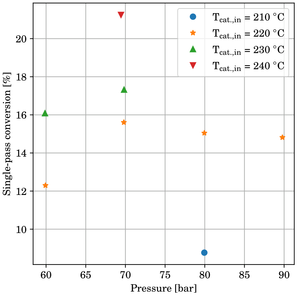
  61. Graaf, G.H.; Stamhuis, E.J.; Beenackers, A.A.C.M. Kinetics of low-pressure methanol synthesis. Chem. Eng. Sci. 1988, 43, 3185–3195. [Google Scholar] [CrossRef]
  62. Vanden Bussche, K.M.; Froment, G.F. A steady-state kinetic model for methanol synthesis and the water gas shift reaction on a commercial Cu/ZnO/Al2O3 catalyst. J. Catal. 1996, 161, 1–10. [Google Scholar] [CrossRef]
  63. Park, N.; Park, M.J.; Lee, Y.J.; Ha, K.S.; Jun, K.W. Kinetic modeling of methanol synthesis over commercial catalysts based on three-site adsorption. Fuel Process. Technol. 2014, 125, 139–147. [Google Scholar] [CrossRef]
  64. Seidel, C.; Jörke, A.; Vollbrecht, B.; Seidel-Morgenstern, A.; Kienle, A. Kinetic modeling of methanol synthesis from renewable resources. Chem. Eng. Sci. 2018, 175, 130–138. [Google Scholar] [CrossRef]
  65. Van Schagen, T.N.; Keestra, H.; Brilman, D.W.F. Improved kinetic model for methanol synthesis with Cu/ZnO/Al2O3 catalysts based on an extensive state-of-the-art dataset. Chem. Eng. J. 2025, 507, 159953. [Google Scholar] [CrossRef]
  66. Lommerts, B.J.; Graaf, G.H.; Beenackers, A.A.C.M. Mathematical modeling of internal mass transport limitations in methanol synthesis. Chem. Eng. Sci. 2000, 55, 5589–5598. [Google Scholar] [CrossRef]
  67. Gunn, D.J. Axial and radial dispersion in fixed beds. Chem. Eng. Sci. 1987, 42, 363–373. [Google Scholar] [CrossRef]
  68. Delgado, J.M.P.Q. A critical review of dispersion in packed beds. Heat Mass Transf. 2006, 42, 279–310. [Google Scholar] [CrossRef]
  69. Yagi, S.; Kunii, D. Studies on effective thermal conductivities in packed beds. AIChE J. 1957, 3, 373–381. [Google Scholar] [CrossRef]
  70. Yagi, S.; Kunii, D.; Wakao, N. Studies on axial effective thermal conductivities in packed beds. AIChE J. 1960, 6, 543–546. [Google Scholar] [CrossRef]
  71. Gmehling, J.; Liu, D.D.; Prausnitz, J.M. High-pressure vapor-liquid equilibria for mixtures containing one or more polar components. Application of an equation of state which includes dimerization equilibria. Chem. Eng. Sci. 1979, 34, 951–958. [Google Scholar] [CrossRef]
  72. Brunner, E.; Hultenschmidt, W.; Schlichtharle, G. Fluid mixtures at high pressures IV. Isothermal phase equilibria in binary mixtures consisting of (methanol + hydrogen or nitrogen or methane or carbon monoxide or carbon dioxide). J. Chem. Thermodyn. 1987, 19, 273–291. [Google Scholar] [CrossRef]
  73. Vogel, K.; Hocke, E.; Beisswenger, L.; Drochner, A.; Etzold, B.J.M.; Vogel, H. Investigation of the Phase Equilibria of CO2/CH3OH/H2O and CO2/CH3OH/H2O/H2 Mixtures. Chem. Eng. Technol. 2019, 42, 2386–2392. [Google Scholar] [CrossRef]
  74. Boston, J.F.; Britt, H.I. A radically different formulation and solution of the single-stage flash problem. Chem. Eng. 1978, 2, 109–122. [Google Scholar] [CrossRef]
Figure 1. Flowsheet used in the steady-state model. Solid arrows represent fluid flow streams, while dashed arrows represent heat flows. H1 denotes the electrical catalyst preheater, R1 denotes the catalyst bed, H2 denotes the tube side of the economizer section, C1 (combined with the first flash vessel) denotes the condenser, H3 denotes the shell side of the economizer section, H4 denotes the shell side around the catalyst bed, and H5 can account for heat losses to the environment in the bottom section of the reactor. The valve with the second flash vessel is a low-pressure flash to determine the amount of dissolved gases in the liquid coming from the reactor.
Chemengineering 10 00062 g001
Figure 2. Model-calculated temperature profile in the reactor compared to experimental data at 60 bar and a catalyst bed inlet temperature of 220 °C. The error bars in the experimental denote twice the standard deviation around the time-averaged value.
Chemengineering 10 00062 g002
Figure 3. Apparent heat transfer coefficient profiles calculated from experimental data at 60 bar and a catalyst bed inlet temperature of 220 °C.
Chemengineering 10 00062 g003
Figure 4. Catalyst bed to shell apparent heat transfer coefficient for the various experiments.
Chemengineering 10 00062 g004
Figure 5. Mean heat integration apparent heat transfer coefficient for the various experiments.
Chemengineering 10 00062 g005
Figure 6. Heat loss apparent heat transfer coefficient for the various experiments.
Chemengineering 10 00062 g006
Figure 7. Model-calculated single-pass carbon conversion for the experiments at varying pressure and catalyst bed inlet temperature.
Chemengineering 10 00062 g007
Figure 8. Model-calculated recycle mass flow compared to the experimental anemometer output for the experiments at varying pressure and catalyst bed inlet temperature. The points (with a black border) show the model mass flow output (left axis), while the error bars show the experimental anemometer output (twice the standard deviation around the time-averaged value) (right axis).
Chemengineering 10 00062 g008
Figure 10. Experimentally measured catalyst bed preheater duty divided by the model-calculated duty.
Chemengineering 10 00062 g010
Figure 11. Experimentally measured condenser duty divided by the model-calculated duty.
Chemengineering 10 00062 g011
Figure 12. Maximum natural convection loop mass flow calculated by Equation (7) divided by the model-calculated loop mass flow.
Chemengineering 10 00062 g012
Figure 13. Model-calculated energy balance over the reactor for the various experiments. The left bar shows the energy sources and the right bar shows the energy sinks. The two bottom parts of the bars correspond to the internal heat integration streams. The hatched areas show heat losses to the environment from the shell side of the reactor.
Chemengineering 10 00062 g013
Figure 14. Minimum temperature difference required for natural convection as a function of the single-pass CO2 conversion with a catalyst bed temperature of 220 °C at 80 bar.
Chemengineering 10 00062 g014
Figure 15. Maximum natural convection flow as a function of the temperature difference between the tube and shell sides, for different single-pass CO2 conversions, with a catalyst bed temperature of 220 °C at 80 bar.
Chemengineering 10 00062 g015
Figure 16. Model-calculated single-pass carbon conversion as a function of the recycle mass flow in the reactor and the pressure.
Chemengineering 10 00062 g016
Figure 17. Model-calculated single-pass carbon conversion as a function of the recycle mass flow in the reactor and the catalyst bed inlet temperature.
Chemengineering 10 00062 g017
Figure 18. Model-calculated single-pass carbon conversion as a function of the recycle mass flow in the reactor and the catalyst bed heat transfer coefficient.
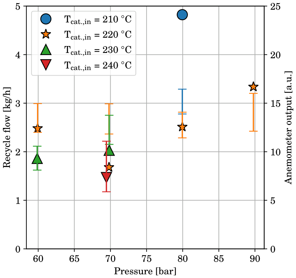
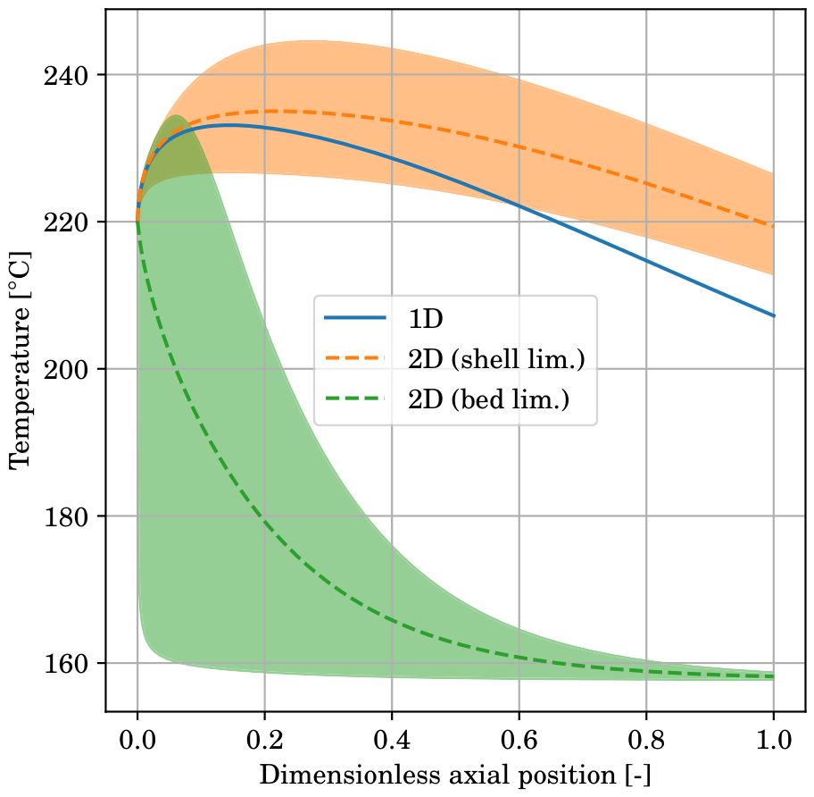
Chemengineering 10 00062 g018
Figure 19. Model-calculated catalyst bed outlet temperature as a function of the recycle mass flow in the reactor and the catalyst bed heat transfer coefficient.
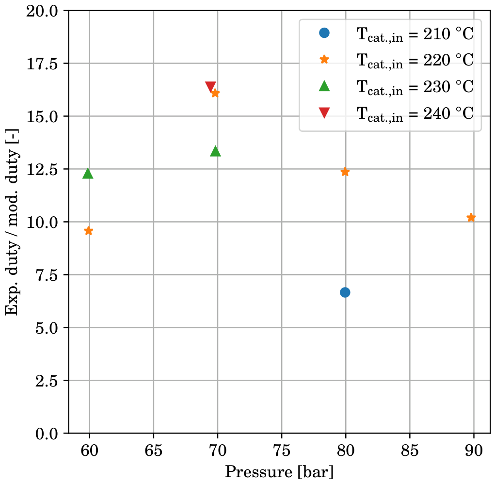
Chemengineering 10 00062 g019
Figure 20. Model-calculated operability range (unhatched area) and space–time yield as a function of the recycle mass flow in the reactor and the pressure at a catalyst bed inlet temperature of 220 °C and a condenser temperature of 40 °C. Note that heat losses to the environment were neglected in these simulations.
Chemengineering 10 00062 g020
Figure 21. Model-calculated operability range (unhatched area) and space–time yield as a function of the recycle mass flow in the reactor and the catalyst bed inlet temperature at a pressure of 75 bar and a condenser temperature of 40 °C. Note that heat losses to the environment were neglected in these simulations.
Chemengineering 10 00062 g021
Figure 22. Model-calculated operability range (unhatched area) and space–time yield as a function of the recycle mass flow in the reactor and the condenser temperature at a pressure of 75 bar and a catalyst bed inlet temperature of 220 °C. Note that heat losses to the environment were neglected in these simulations.
Chemengineering 10 00062 g022
Table 1. Parameters used in the steady-state model and their default values or source. The tag numbers refer to the P&ID of the experimental setup; see van Schagen et al. [31].
ParameterRelevant Stream/UnitValue/Source
Feed H2 flowStream 1FT510
Feed CO2 flowStream 1FT520
Feed temperatureStream 1TT542
Pressure-PT550
Catalyst inlet temperatureH1TT552
Catalyst amountR1383 g
Catalyst bed lengthR1/H415 cm
Catalyst particle diameterR15.0 mm
Catalyst particle densityR11300 kg m−3
Catalyst bed porosityR10.40
Bed to shell heat transfer coefficientR1/H4(Equation (8))
Economizer lengthH2/H31.25 m
Economizer heat transfer coefficientH2/H3(Equation (8))
Economizer heat loss coefficientH2/H3(Equation (8))
Condenser lengthC10.20 m
Condenser heat transfer coefficientC1300 W m−2 K−1
Condenser temperatureC1TT555
Purge fractionSP10.10%
Total vertical length-2.0 m
Ambient temperature-20 °C
Table 2. Fitted linear correlations for the apparent heat transfer coefficients as a function of the recycle mass flow.
LocationSlope [Wm−2K−1kg−1h]Intercept [Wm−2K−1]
Catalyst bed8.04.3
Economizer3.11.8
Heat losses2.72.1
Disclaimer/Publisher’s Note: The statements, opinions and data contained in all publications are solely those of the individual author(s) and contributor(s) and not of MDPI and/or the editor(s). MDPI and/or the editor(s) disclaim responsibility for any injury to people or property resulting from any ideas, methods, instructions or products referred to in the content.