
Partial Order as Decision Support between Statistics and Multicriteria Decision Analyses


Abstract
1. Introduction
1.1. An Exemplary Case
- a simultaneous consideration of all three indicators is performed, i.e., independent of the specific indicator, and
- no aggregation to form a composite indicator is applied, and hence no weights are necessary.
A First (Preliminary) Conclusion
2. An Attempt for a Positioning of Partial Order
- The objective of any MCDA method is a ranking construct (by different and often highly sophisticated techniques) requiring a ranking index, which is a scalar as only a scalar can assure the absence of incomparabilities. Nevertheless, a scalar does not necessarily prevent the presence of nontrivial equivalence classes, and even if the unwanted effect of incomparabilities is avoided, the construction of a scalar from indicator values must take care to reduce as much as possible the ties with respect to the values of the scalar. However, the main point of construction of a scalar is the fact that incomparabilities are suppressed, although such incomparabilities indicate severe conflicts among the options or objects; disclosure of these conflicts should not be ignored.
- Any aggregation, mapping m indicators onto a one-dimensional scalar, such as one of the ci’s above, ignores specific information of the single indicators. In the final sequence, in ci1 it is no more evident that IRE is good with respect to wb and hs but strikingly bad with respect to br, which should evoke specific management plans. IRE is independent of the weight regime at the top of the sequences (2)–(4).
- The construction of a scalar is necessarily a mapping of a multidimensional system onto a one-dimensional quantity. Then, depending on the technical form of construction, compensation effects may develop [Munda, 2008], i.e., favorable indicator values may compensate for unfavorable ones. Accepting that partial order can deliver incomparabilities also means that in such cases compensation is conceptually eliminated; furthermore, conflicts are brought into the light. In light of the example above: IRE needs no management because IRE is at the top of sequence (2) (and the other two). Nevertheless, IRE has a deficit in br. This deficit is balanced out (compensated for) by the two good values in wb and hs.
2.1. Partial Order in Its Application on Multi-Indicator Systems (MIS)—An Attempt for a Localization within the Context of Other Mathematical Disciplines
Three Pillars of Statistics and the Partial Order Counterpart
- Descriptive statisticsPartial order (in its application to MIS) is based on standard statistics and does not add (at least up to now) its own concepts.
- Explorative statisticsPartial order can explore data as to how much they contribute to a ranking. The background is its graph theoretical basis, which consequently leads to the question of why the graph induced by partial order has certain structures.
- Inference statisticsInference methods aim at a decision as to how far results from certain random sampling or spot tests can be extended to a universe. This important question should also be transferred to partial order applications. However, there the focus is on the objects for which a decision is to be found, and not on the generalization. Nevertheless, first attempts to judge the role of noise within partial order can be found in [20]. At least it cannot be claimed that a test theory in partial order applications is at hand.
3. Basic Concepts of Partial Order in Application on MIS
3.1. Basic Equation
- Objects: the items for which a decision is to be found, i.e., for which a ranking is the objective.
- Indicators: as most often the ranking objective, for example urban quality, cannot be directly measured, a set of indicators is defined that describe the important aspects of the wanted ranking. As several indicators are needed (as in the example above six indicators for child well-being), a multi-indicator system (MIS) is consequently found.
3.2. Important Notations
- Maximal element: If there is no y for which y > x is valid, then x is called a maximal element.
- Minimal element: If there is no y for which y < x is valid, then x is called a minimal element.
- If there is only one maximal (minimal) element, then this element is called a greatest (least) element.
- If x is at the same time a maximal and a minimal element, it is called an isolated element (from an explorative point of view, isolated elements indicate interesting data structures).
- Let X be the set of all objects of a study. Then X′ as a subset of X is called a chain if for every element of X′ it is found x < y or x > y.
- X″ is a subset of X called an antichain if for any two objects taken from X″ an incomparability is found.
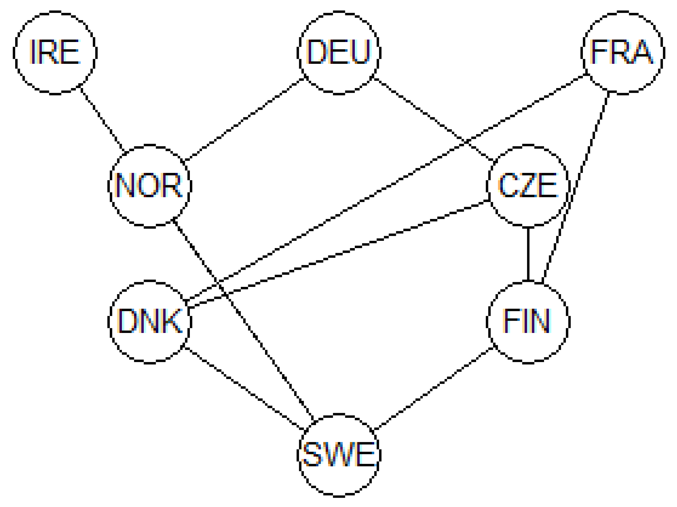
- IRE, DEU and FRA are maximal elements
- SWE is a minimal element: it is a least element because it is the only nation that is a minimal element.
- {SWE, DNK, DE, CZE} is an example of a chain. Indeed, it is found: SWE < DNK < CZE < DE
- {NOR, CZE, FRA} is one example of an antichain. Indeed, Equation (6) cannot be applied for any pair of objects taken from this subset.
3.3. Generalized Linear Aggregation
4. Software
5. Selected Examples of the Application of Partial Ordering
5.1. Novichok—Why the Skripals Did Not Die

5.2. Stakeholders/Decision Makers Influence
5.3. Peculiar Elements/Outliers
5.4. Formal Concept Analyses
- (1)
- the implication is to be considered a hypothesis, as it is only related to a sample;
- (2)
- any implication urgently needs a contextual interpretation;
- (3)
- any other discretization, say to d values, can change the result.
6. Conclusions and Outlook
6.1. Conclusions
- Comparability: An increase in an indicator value is always accompanied by a non-decrease of all other indicators. For decision making, an overwhelming number of comparabilities is a comfortable situation, as a ranking is almost found. When all n objects are mutually comparable, then the limit of a ranking is reached.
- Incomparabilty: An increase in the values of some indicators is accompanied by a decrease of some others. This expresses a conflict because a preferred state due to some indicators is weakened by unpreferred values of other indicators. The evidence of conflicts is smashed out by aggregation methods to obtain a single quantity, which allows a ranking. However, in a public audit there is a great deal of resistance explainable by the loss of information about the inherent conflicts.
- an advantage, because they can be understood, but they have three
- disadvantages, namely:
- ○
- compensation effects,
- ○
- uncertainty in the weights themselves, “Is aspect x really more important than aspect y?”, and
- ○
- need of a numerical representation of qualitative knowledge by weights.
6.2. Limitations and Outlook
- (1)
- The problem of noisy data is algorithmically solved; however, there is still the need of tests guaranteeing that there is a high probability for typical partial order theoretical results, such as “being a maximal element”. Up to now, only the relational point of view is considered. However, when the data matrix has noisy data, then there must be a statement possible such as: There is a probability of, e.g., p% that an object is a maximal element.
- (2)
- The above-mentioned problem of the scaling level of data. This problem can be circumvented by establishing preference functions (as done in many MCDA methods). Accepting the need to establish preference functions opens the door to many subsequent questions, such as: Which kind of preference function? How robust is the preference function in a statistical sense?
- (3)
- When partial order is applied on a MIS (without the use of matrix G), then the interpretation of incomparabilities can be directly traced back to single indicator values. However, when a new MIS is constructed in accordance with Equation (7), remaining incomparabilities are caused by two influences: (a) indicator values and (b) weights. An attempt to solve this problem is under work.
- (4)
- Partial order theory provides its own concept to obtain a weak order (average ranking). Although this concept is not specifically mentioned here, it plays a role as a mean for comparisons. How far does final ranking coincide with that provided by partial ordering? When this question appears, a subsequent problem arises: How far is any approximative construction of linear orders out of a poset exact? An exact linear ordering is most often computationally not tractable; hence, good approximations are needed.
- (5)
- Partial order theory delivers mathematical concepts. Many of them seem to have a seed for useful application with MIS. Identifying these and checking their role for application with MIS is a permanent task, as mathematicians really do not sleep!
7. Further Reading
Author Contributions
Funding
Institutional Review Board Statement
Informed Consent Statement
Data Availability Statement
Conflicts of Interest
Appendix A
| Country | d1 | d2 | d3 | d4 | d5 | d6 | d7 | d8 | d9 | d10 | d11 | d12 |
| Cyprus | 4 | 4.5 | 7 | 4.5 | 6.4 | 6.7 | 5.3 | 3 | 3.3 | 4.4 | 7.9 | 9.2 |
| Bulgaria | 4.2 | 3.5 | 5.2 | 4.6 | 4.9 | 6.2 | 5 | 4.2 | 3.4 | 4.1 | 5.3 | 4.8 |
| Romania | 3.7 | 2.7 | 6.8 | 4.5 | 4.7 | 5.2 | 5.6 | 4.3 | 3.9 | 3.5 | 5.2 | 4.1 |
| Greece | 3.6 | 1.6 | 5 | 3.8 | 4.2 | 6.5 | 6.5 | 3.9 | 3.4 | 4.5 | 3.7 | 5.9 |
| Croatia | 3.6 | 4.9 | 5.7 | 4.5 | 3.8 | 5.3 | 3.4 | 2.9 | 4.1 | 4 | 4.4 | 4.4 |
| Hungary | 2.3 | 2.5 | 4.7 | 3.3 | 4.3 | 5.9 | 6.6 | 3.3 | 4.5 | 2.4 | 5.3 | 4 |
| Latvia | 3.4 | 2.9 | 7.4 | 4.4 | 4.6 | 4 | 3.9 | 3.4 | 3 | 3.5 | 4.3 | 3.8 |
| Estonia | 3.3 | 2.9 | 6.5 | 3.5 | 3.7 | 3.6 | 3.2 | 3.4 | 2 | 3.1 | 5.5 | 3.1 |
| Italy | 3.1 | 3.7 | 4.9 | 2 | 3.4 | 5.6 | 4.2 | 2.3 | 2.5 | 4.4 | 4.9 | 2.2 |
| Lithuania | 3.3 | 2.6 | 4.3 | 4.2 | 5 | 5 | 3.2 | 4 | 2.4 | 3 | 3 | 3 |
| Slovakia | 2.8 | 2 | 5.9 | 4.2 | 4 | 5.1 | 3.7 | 2.9 | 2.7 | 2.3 | 3.7 | 3.3 |
| Malta | 2.8 | 4.6 | 3.9 | 4 | 2.9 | 4.2 | 3.9 | 2.3 | 3.3 | 3.4 | 2 | 3.6 |
| Spain | 2.5 | 1.7 | 5.8 | 2.4 | 4 | 5 | 3.3 | 2.7 | 1.9 | 3.3 | 6.1 | 2.2 |
| Poland | 3.3 | 2.8 | 4.4 | 4.4 | 3.5 | 4.1 | 3.2 | 2.8 | 2.5 | 2.3 | 3.8 | 2.7 |
| Czech Rep. | 1.9 | 2 | 3.8 | 2.8 | 3.2 | 4.8 | 4.2 | 3.1 | 2.1 | 2.6 | 4.3 | 2.6 |
| France | 2.8 | 2.2 | 6.8 | 2.2 | 3.7 | 4.8 | 1.8 | 1.5 | 2.3 | 2.3 | 1.9 | 1.4 |
| United King. | 2.6 | 2.4 | 5.6 | 2.1 | 3.7 | 3.9 | 2 | 2.1 | 1.8 | 2.5 | 3.5 | 1.2 |
| Slovenia | 2.8 | 1.4 | 3.9 | 2.8 | 3.9 | 4.2 | 2.6 | 2 | 2 | 2.1 | 1.6 | 2.3 |
| Belgium | 2.5 | 1.6 | 4.1 | 1.9 | 3.2 | 4.5 | 1.9 | 2.1 | 1.2 | 2 | 3.9 | 1.5 |
| Portugal | 2.6 | 1.6 | 2.6 | 2.2 | 2.9 | 5.1 | 1.8 | 2.7 | 2.3 | 1.6 | 1.8 | 2.5 |
| Germany | 2.5 | 3 | 4.6 | 2.1 | 3.3 | 2.9 | 1.2 | 1.6 | 1.5 | 2.1 | 2 | 1.3 |
| Netherlands | 3 | 2.1 | 3.9 | 2.6 | 2.7 | 3.4 | 1 | 1.5 | 1 | 1.8 | 2.6 | 1.2 |
| Austria | 2.4 | 2 | 4.3 | 1.5 | 3.4 | 2.2 | 1.4 | 1.6 | 1.7 | 1.1 | 2.7 | 1.7 |
| Ireland | 2.2 | 1.4 | 1.9 | 2.8 | 2.7 | 4.1 | 1.5 | 1.9 | 1.2 | 1.8 | 1.3 | 1.9 |
| Luxembourg | 1.7 | 1.7 | 3.1 | 2.1 | 1.5 | 1.5 | 1.3 | 1.3 | 1 | 2 | 3.4 | 1.6 |
| Denmark | 2.5 | 1.4 | 3.6 | 1.9 | 2.1 | 2.5 | 0.5 | 1.4 | 1.3 | 1.5 | 1.4 | 1.4 |
| Norway | 2.5 | 2.3 | 1.3 | 1.5 | 1.8 | 2.3 | 1 | 1.6 | 1 | 2.1 | 1.8 | 1 |
| Sweden | 1.5 | 1.5 | 1.6 | 2.3 | 1 | 3.8 | 0.5 | 1.2 | 0.9 | 1.4 | 1.1 | 1 |
Appendix B
| Country | d1 | d2 | d3 | d4 | d5 | d6 | d7 | d8 | d9 | d10 | d11 | d12 |
| Cyprus | 1 | 1 | 1 | 1 | 1 | 1 | 1 | 1 | 1 | 1 | 1 | 1 |
| Bulgaria | 1 | 1 | 1 | 1 | 1 | 1 | 1 | 1 | 1 | 1 | 1 | 1 |
| Romania | 1 | 1 | 1 | 1 | 1 | 1 | 1 | 1 | 1 | 1 | 1 | 1 |
| Greece | 1 | 0 | 1 | 1 | 1 | 1 | 1 | 1 | 1 | 1 | 1 | 1 |
| Croatia | 1 | 1 | 1 | 1 | 1 | 1 | 1 | 1 | 1 | 1 | 1 | 1 |
| Hungary | 0 | 1 | 1 | 1 | 1 | 1 | 1 | 1 | 1 | 0 | 1 | 1 |
| Latvia | 1 | 1 | 1 | 1 | 1 | 0 | 1 | 1 | 1 | 1 | 1 | 1 |
| Estonia | 1 | 1 | 1 | 1 | 1 | 0 | 1 | 1 | 0 | 1 | 1 | 1 |
| Italy | 1 | 1 | 1 | 0 | 0 | 1 | 1 | 0 | 1 | 1 | 1 | 0 |
| Lithuania | 1 | 1 | 0 | 1 | 1 | 1 | 1 | 1 | 1 | 1 | 0 | 1 |
| Slovakia | 0 | 0 | 1 | 1 | 1 | 1 | 1 | 1 | 1 | 0 | 1 | 1 |
| Malta | 0 | 1 | 0 | 1 | 0 | 0 | 1 | 0 | 1 | 1 | 0 | 1 |
| Spain | 0 | 0 | 1 | 0 | 1 | 1 | 1 | 1 | 0 | 1 | 1 | 0 |
| Poland | 1 | 1 | 0 | 1 | 0 | 0 | 1 | 1 | 1 | 0 | 1 | 0 |
| Czech Rep | 0 | 0 | 0 | 0 | 0 | 1 | 1 | 1 | 0 | 0 | 1 | 0 |
| France | 0 | 0 | 1 | 0 | 1 | 1 | 0 | 0 | 1 | 0 | 0 | 0 |
| United King. | 0 | 0 | 1 | 0 | 1 | 0 | 0 | 0 | 0 | 0 | 0 | 0 |
| Slovenia | 0 | 0 | 0 | 0 | 1 | 0 | 0 | 0 | 0 | 0 | 0 | 0 |
| Belgium | 0 | 0 | 0 | 0 | 0 | 1 | 0 | 0 | 0 | 0 | 1 | 0 |
| Portugal | 0 | 0 | 0 | 0 | 0 | 1 | 0 | 1 | 1 | 0 | 0 | 0 |
| Germany | 0 | 1 | 1 | 0 | 0 | 0 | 0 | 0 | 0 | 0 | 0 | 0 |
| Netherlands | 1 | 0 | 0 | 0 | 0 | 0 | 0 | 0 | 0 | 0 | 0 | 0 |
| Austria | 0 | 0 | 0 | 0 | 0 | 0 | 0 | 0 | 0 | 0 | 0 | 0 |
| Ireland | 0 | 0 | 0 | 0 | 0 | 0 | 0 | 0 | 0 | 0 | 0 | 0 |
| Luxembourg | 0 | 0 | 0 | 0 | 0 | 0 | 0 | 0 | 0 | 0 | 0 | 0 |
| Denmark | 0 | 0 | 0 | 0 | 0 | 0 | 0 | 0 | 0 | 0 | 0 | 0 |
| Norway | 0 | 0 | 0 | 0 | 0 | 0 | 0 | 0 | 0 | 0 | 0 | 0 |
| Sweden | 0 | 0 | 0 | 0 | 0 | 0 | 0 | 0 | 0 | 0 | 0 | 0 |
References
- Figueira, J.; Greco, S.; Ehrgott, M. Multiple Criteria Decision Analysis, State of the Art Surveys; Springer: Boston, MA, USA, 2005. [Google Scholar]
- Brans, J.P.; Vincke, P.H.A. Preference Ranking Organisation Method (The PROMETHEE Method for Multiple Criteria Decision-Making). Manag. Sci. 1985, 31, 647–656. [Google Scholar] [CrossRef]
- Brans, J.P.; Vincke, P.H.; Mareschal, B. How to select and how to rank projects: The PROMETHEE method. Eur. J. Oper. Res. 1986, 24, 228–238. [Google Scholar] [CrossRef]
- Brans, J.P.; Mareschal, B. The PROMCALC & GAIA decision support system for multicriteria decision aid. Decis. Support Syst. 1994, 12, 297–310. [Google Scholar]
- Li, H.; Wang, J. An Improved Ranking Method for ELECTRE III. In Proceedings of the International Conference on Wireless Communications, Networking and Mobile Computing, Shanghai, China, 21–25 September 2007; pp. 6659–6662. [Google Scholar]
- Saaty, T.L. How to Make a Decision: The Analytical Hierarchy Process. Interfaces 1994, 24, 19–43. [Google Scholar] [CrossRef]
- Brüggemann, R.; Patil, G.P. Ranking and Prioritization for Multi-Indicator Systems—Introduction to Partial Order Applications; Springer: New York, NY, USA, 2011. [Google Scholar]
- Order. A Journal on the Theory of Ordered Sets and Its Applications. Available online: https://www.springer.com/journal/11083 (accessed on 1 January 2022).
- UNICEF. Child Poverty in Perspective: An Overview of Child Well-Being in Rich Countries; Innocenti Report Card7; UNICEF Innocenti Research Centre: Florence, Italy, 2007. [Google Scholar]
- Roy, B.; Vanderpooten, D. The European School of MCDA: Emergence, Basic Features and Current Works. J. Multi-Criteria Decis. Anal. 1996, 5, 22–38. [Google Scholar] [CrossRef]
- Fishburn, P.C. Utility Theory for Decision Making; John Wiley & Sons, Inc.: New York, NY, USA, 1970. [Google Scholar]
- Firshburn, P.C. Research in Decision Theory: A Personal Perspective. Math. Soc. Sci. 1983, 5, 129–148. [Google Scholar] [CrossRef]
- Gomes, L.F.A.M.; Rangel, L.A.D. An Application of the TODIM method to the multicriteria rental evaluation of residental properties. Eur. J. Oper. Res. 2009, 193, 204–211. [Google Scholar] [CrossRef]
- Erné, M. Einführung in Die Ordnungstheorie; Deutsche Digitale Bibliotek: 1982. Available online: https://www.deutsche-digitale-bibliothek.de/item/JQ2CJEO4N7X6E4V6FDSG3YXKGXGHBSQP (accessed on 1 January 2022).
- Dedekind, R. Über die von drei Modulen erzeugte Dualgruppe. Math. Ann. 1900, 53, 371–403. [Google Scholar] [CrossRef]
- Dedekind, R. Was Sind und Was Sollen Die Zahlen? 10th ed.; Vieweg: Braunschweig, Germany, 1969. [Google Scholar]
- Birkhoff, G. Lattice Theory, 3rd ed.; American Mathematical Socienty: Providence, RI, USA, 1973. [Google Scholar]
- Hasse, H. Vorlesungen über Klassenkörpertheorie; Physica-Verlag: Wurzburg, Germany, 1967. [Google Scholar]
- Halfon, E.; Reggiani, M.G. On Ranking Chemicals for Environmental Hazard. Environ. Sci. Technol. 1986, 20, 1173–1179. [Google Scholar] [CrossRef]
- Bruggemann, R.; Carlsen, L. An attempt to Understand Noisy Posets. MATCH Commun. Math. Comput. Chem. 2016, 75, 485–510. [Google Scholar]
- Ganter, B.; Ille, R. Formale Begriffsanalyse-Mathematische Grundlagen; Springer: Berlin/Heidelberg, Germany, 1996; pp. 1–282. [Google Scholar]
- Wille, R. Concept Lattices and Conceptual Knowledge Systems. Comput. Math. Appl. 1992, 23, 493–515. [Google Scholar] [CrossRef]
- Carpineto, C.; Romano, G. Concept Data Analysis: Theory and Applications; Wiley: Chichester, UK, 2004. [Google Scholar]
- Kerber, A.; Brüggemann, R. Problem Orientable Evaluations as L-subsets. In Measuring and Understanding Complex Phenomena; Indicators and Their Analysis in Different Scientific Fields; Brüggemann, R., Carlsen, L., Beycan, T., Suter, C., Maggino, F., Eds.; Springer Nature: Cham, Switzerland, 2021; pp. 83–89. [Google Scholar]
- Brüggemann, R.; Carlsen, L.; Voigt, K.; Wieland, R. PyHasse Software for Partial Order Analysis. In Multi-Indicator Systems and Modelling in Partial Order; Bruggemann, R., Carlsen, L., Wittmann, J., Eds.; Springer: New York, NY, USA, 2014; pp. 389–423. [Google Scholar]
- Brüggemann, R.; Kerber, A.; Koppatz, P.; Pratz, V. PyHasse, a Software Package for Application Studies of Partial Orderings. In Measuring and Understanding Complex Phenomena; Indicators and Their Analysis in Different Scientific Fields; Brüggemann, R., Carlsen, L., Beycan, T., Suter, C., Maggino, F., Eds.; Springer Nature: Cham, Switzerland, 2021; pp. 291–307. [Google Scholar]
- Arcagni, A. PARSEC: An R Package for Partial Orders in Socio-Economics. In Partial Order Concepts in Applied Sciences; Bruggemann, R., Fattore, M., Eds.; Springer: Cham, Switzerland, 2017; pp. 275–289. [Google Scholar]
- Arcagni, A.; Avellone, A.; Fattore, M. POSetR: A new computationally efficient R package for partially ordered data. In Book of Short Papers—SIS2021; Perna, C., Salvati, N., Spagnolo, F.S., Eds.; Pearson: London, UK, 2021. [Google Scholar]
- Carlsen, L. After Salisbury. Nerve agents revisited. Mol. Inform. 2019, 38, 1800106. [Google Scholar] [CrossRef] [PubMed]
- Bruggemann, R.; Carlsen, L. Incomparable—What now? MATCH-Commun. Math. Comput. Chem. 2014, 71, 694–716. [Google Scholar]
- Carlsen, L.; Bruggemann, R. Gender equality in Europe. The development of the Sustainable Development Goal No. 5 illustrated by exemplary cases. Soc. Ind. Res. 2021, 158, 1127–1151. [Google Scholar] [CrossRef]
- Bruggemann, R.; Kerber, A. Evaluations as Sets over Lattices—Application point of view. In Measuring and Understanding Complex Phenomena; Indicators and Their Analysis in Different Scientific Fields; Brüggemann, R., Carlsen, L., Beycan, T., Suter, C., Maggino, F., Eds.; Springer Nature: Cham, Switzerland, 2021; pp. 91–101. [Google Scholar]
- Fragile States Index, Fund for Peace. 2015. Available online: https://fragilestatesindex.org/2015/06/17/fragile-states-index-2015-annual-report/ (accessed on 1 January 2022).
- Methodology behind Cast, Fund for Peace. 2006. Available online: http://www.fundforpeace.org/cast/index.php?option=com_content&task=view&id=14&Itemid=30 (accessed on 1 January 2022).
- Baker, P.H. Conflict Assessment System Tool (CAST). An Analytical Model for Early Warning and Risk Assessment of Weak and Failing States; The Fund for Peace: Washington, WA, USA, 2006; Available online: http://www.fundforpeace.org/cast/pdf_downloads/castmanual2007.pdf (accessed on 1 January 2022).
- Fund for Peace. Conflict Assessment Indicators. The Fund for Peace Country Analysis Indicators and Their Measures; The Fund for Peace Publication CR-10-97-CA (11-05C); Fund for Peace: Washington, WA, USA, 2011; Available online: http://www.fundforpeace.org/global/library/cr-10-97-ca-conflictassessmentindicators-1105c.pdf (accessed on 1 January 2022).
- Aigner, M. Producing posets. Discret. Math. 1981, 35, 1–15. [Google Scholar] [CrossRef]
- Aigner, M. Uses of the Diagram Lattice. Mitt. Math. Sem. Univ. Giess. 1984, 103, 61–77. [Google Scholar]
- Brightwell, G.R. Partial Orders. In Graph Connections Relationships between Graph Theory and Other Areas of Mathematics; Beineke, L.W., Wilson, R.J., Eds.; Clarendon Press: Oxford, UK, 1997; pp. 52–69. [Google Scholar]
- Brightwell, G.R.; West, D.B. Partially ordered Sets. In Handbook of Discrete and Combinatorial Mathematics; Rosen, K.R., Ed.; CRC Press: Boca Raton, FL, USA, 2000; pp. 717–752. [Google Scholar]
- Barthelemy, J.P.; Flament, C.; Monjardet, B. Ordered sets and social sciences. In Ordered Sets NATO Advanced Study Institutes Series C: Mathematical and Physical Sciences C83; Rival, I., Ed.; Reidel Publishing Company: Dordrecht, Germany, 1982; pp. 721–758. [Google Scholar]
- Bouyssou, D.; Vincke, P. Binary relations and preference modeling. In Decision Making Process: Concepts and Methods; Bouyssou, D., Dubois, D., Prade, H., Pirlot, M., Eds.; Wiley: New York, NY, USA, 2009; pp. 49–84. [Google Scholar]
- Carlsen, L.; Bruggemann, R. On the influence of data noise and uncertainty on ordering of objects, described by a multi-indicator system. A set of pesticides as an exemplary case. J. Chemom. 2016, 30, 22–29. [Google Scholar] [CrossRef]
- Hasse, H. Höhere Algebra II Gleichungen höheren Grades; Bei de Gruyter: Berlin, Germany, 1927. [Google Scholar]
- Hyde, K.; Maier, H.R.; Colby, C. Incorporating uncertainty in the PROMETHEE MCDA method. J. Multi-Criteria Decis. Anal. 2003, 12, 245–259. [Google Scholar] [CrossRef]
- Meyer, P.; Olteanu, A.L. Formalizing and solving the problem of clustering in MCDA. Eur. J. Oper. Res. 2013, 227, 494–502. [Google Scholar] [CrossRef]
- Panahbehagh, B.; Bruggemann, R. Introduction into Sampling Theory, Applying Partial Order Concepts. In Measuring and Understanding Complex Phenomena; Indicators and Their Analysis in Different Scientific Fields; Bruggemann, R., Carlsen, L., Beycan, T., Suter, C., Maggino, F., Eds.; Springer Nature: Cham, Switzerland, 2021; pp. 135–151. [Google Scholar]
- Rival, I. Ordered Sets; Reidel Publishing Company: Dordrecht, Germany, 1982. [Google Scholar]
- Restrepo, G.; Bruggemann, R. Ranking Regions using cluster analysis, Hasse diagram technique and topology. In Proceedings of the 3rd International Congress on Environmental Modelling and Software, Brigham Young University BYU Scholars Archive, Burlington, VT, USA, 9–13 July 2006. [Google Scholar]
- Sałabun, W.; Wątróbski, J.; Shekhovtsov, A. Are MCDA Methods Benchmarkable? A Comparative Study of TOPSIS, VIKOR, COPRAS, and PROMETHEE II Methods. Symmetry 2020, 12, 1549. [Google Scholar] [CrossRef]
- Trotter, W.T. Combinatorics and Partially Ordered Sets, Dimension Theory; The Johns Hopkins University Press: Baltimore, MD, USA, 1992. [Google Scholar]
- Winkler, P. Average height in a partially ordered set. Discret. Math. 1982, 39, 337–341. [Google Scholar] [CrossRef]
- Xu, B.; Ouenniche, J. Performance evaluation of competing forecasting models: A multidimensional framework based on MCDA. Expert Syst. Appl. 2012, 39, 8312–8324. [Google Scholar] [CrossRef]
- Abbas, A.E. Invariant Utility Functions and Certain Equivalent Transformations. Decis. Anal. 2007, 4, 17–31. [Google Scholar] [CrossRef]
- Cardoso, D.M.; de Sousa, J.F. A Numerical Tool for Multiattribute Ranking Problems. Networks 2003, 41, 229–234. [Google Scholar] [CrossRef]
- Al-Sharrah, G. Ranking Using the Copeland Score: A Comparsion with the Hasse Diagram. J. Chem. Inf. Model. 2010, 50, 785–791. [Google Scholar] [CrossRef]
- da Silva Monte, M.B.; De Almeida Filho, A.T. A MCDM model for preventive maintenance on wells for water distribution. In Proceedings of the 2015 IEEE International Conference on Systems, Man, and Cybernetics, Hong Kong, China, 9–12 October 2015; pp. 268–272. [Google Scholar]
- de Carvalho, V.D.H.; Poleto, T.; Nepomuceno, T.C.C.; Costa, A.P.P.C.S. A study on relational factors in information technology outsourcing: Analyzing judgments of small and medium-sized supplying and contracting companies’ managers. J. Bus. Ind. Mark. 2022, 37, 893–917. [Google Scholar] [CrossRef]
- de Carvalho, V.D.H.; Poleto, T.; Seixas, A.P.C. Information technology outsourcing relationship integration: A critical success factors study based on ranking problems (P.γ) and correlation analysis. Expert Syst. 2018, 35, e12198. [Google Scholar] [CrossRef]
- Fishburn, P.C. Utility Theory and Decision Theory. In Utility and Probability. The New Palgrave; Eatwell, J., Milgate, M., Newman, P., Eds.; Palgrave Macmillan: London, UK, 1990; pp. 303–312. [Google Scholar]
- Frej, E.A.; de Almeida, A.T.; Costa, A.P.C.S. Using data visualization for ranking alternatives with partial information and interactive tradeoff elicitation. Oper. Res. 2019, 19, 909–931. [Google Scholar] [CrossRef]
- Lootsma, F.A. Multi-Criteria Decision Analysis and Multi-Objective Optimization; TU Delft: Delft, The Netherlands, 1996. [Google Scholar]
- Munda, G. Multiple-Criteria Decision Aid: Some Epistemological Considerations. J. Multi-Criteria Decis. Anal. 1993, 2, 41–55. [Google Scholar] [CrossRef]
- Munda, G. Social Multi-Criteria Evaluation for a Sustainable Economy; Springer: Berlin, Germany, 2008. [Google Scholar]
- Munda, G.; Nardo, M. Noncompensatory/nonlinear composite indicators for ranking countries: A defensible setting. Appl. Econ. 2009, 41, 1513–1523. [Google Scholar] [CrossRef]
- Nardo, M. Handbook on Constructing Composite Indicators—Methodology and User Guide; OECD: Ispra, Italy, 2008. [Google Scholar]
- Pudenz, S.; Bruggemann, R.; Lühr, H.-P. Order Theoretical Tools in Environmental Sciences and Decision Systems. In Proceedings of the Third Workshop, Berlin, Germany, 6–7 November 2000; Berichte des IGB, IGB Berlin, Heft 14. Leibniz Institute of Fresh Water Ecology and Inland Fisheries: Berlin, Germany, 2001; pp. 1–224. [Google Scholar]
- Roy, B. Electre III: Un Algorithme de classements fonde sur une representation floue des Preferences en presence de criteres multiples. Cah. Cent. D’etudes Rech. Oper. 1978, 20, 3–24. [Google Scholar]
- Strassert, G. Das Abwägungsproblem bei Multikriteriellen Entscheidungen—Grundlagen und Lösungsansatz unter Besonderer Berücksichtigung der Regionalplanung; Lang: Frankfurt am Main, Germany, 1995. [Google Scholar]
- Vincke, P.H. Robust and Neutral methods for aggregating preferences into an outranking relation. Eur. J. Oper. Res. 1999, 112, 405–412. [Google Scholar] [CrossRef]
- Ade, M.; Bruggemann, R.; Mess, A.; Frahnert, S. Organismische Biologie als Grundlage für die Bewertung von Umweltauswirkungen durch Eingriffe in die Landschaft—Pilotstudie mit Hilfe der Hasse-Diagramm-Technik. UWSF-Z. Umweltchem. Ökotox. 2004, 16, 105–112. [Google Scholar] [CrossRef]
- Bartel, H.-G. Formale Begriffsanalyse und Materialkunde: Zur Archäometrie altägyptischer glasartiger Produkte. MATCH Commun. Math. Comput. Chem. 1995, 32, 27–46. [Google Scholar]
- Bruggemann, R.; Voigt, K. A New Tool to Analyze Partially Ordered Sets. Application: Ranking of polychlorinated biphenyls and alkanes/alkenes in river Main, Germany. MATCH Commun. Math. Comput. Chem. 2011, 66, 231–251. [Google Scholar]
- Bruggemann, R.; Scherb, H.; Schramm, K.-W.; Cok, I.; Voigt, K. CombiSimilarity, an innovative method to compare environmental and health data sets with different attribute sizes example: Eighteen Organochlorine Pesticides in soil and human breast milk samples. Ecotoxicol. Environ. Saf. 2014, 105, 29–35. [Google Scholar] [CrossRef]
- Carlsen, L. Data analyses by partial order methodology. Chem. Bull. Kazakh Natl. Univ. 2015, 78, 22–34. [Google Scholar] [CrossRef][Green Version]
- Carlsen, L. A posetic based assessment of atmospheric VOCs. AIMS Environ. Sci. 2017, 4, 403–416. [Google Scholar] [CrossRef]
- Carlsen, L.; Bruggemann, R. Partial order methodology: A valuable tool in chemometrics. J. Chemom. 2014, 28, 226–234. [Google Scholar] [CrossRef]
- De Loof, K.; De Baets, B.; De Meyer, H.; Brüggemann, R. A Lattice-Theoretic Approach to Computing Averaged Ranks Illustrated on Pollution Data in Baden-Württemberg. In Environmental Informatics and Systems Research; Hryniewicz, O., Studzinski, J., Romaniuk, M., Eds.; Shaker Verlag: Aachen, Germany, 2007; pp. 177–179. [Google Scholar]
- De Loof, K.; De Baets, B.; De Meyer, H.; Bruggemann, R. A Hitchhiker’s Guide to Poset Ranking. Comb. Chem. High Throughput Screen. 2008, 11, 734–744. [Google Scholar] [CrossRef]
- Duchowicz, P.R.; Castro, E.A. The Order Theory in QSPR-QSAR Studies; University of Kragujevac, Faculty of Science: Kragujevac, Serbia, 2008. [Google Scholar]
- El-Basil, S. Partial Ordering of Properties: The Young Diagram Lattice and Related Chemical Systems. In Partial Order in Environmental Sciences and Chemistry; Bruggemann, R., Carlsen, L., Eds.; Springer: Berlin, Germany, 2006; pp. 3–26. [Google Scholar]
- Halfon, E. Is there a best model structure ? I: Modelling the fate of a toxic substance in a lake. Ecol. Model. 1983, 20, 135–152. [Google Scholar] [CrossRef]
- Helm, D. Evaluation of Biomonitoring Data. In Partial Order in Environmental Sciences and Chemistry; Bruggemann, R., Carlsen, L., Eds.; Springer: Berlin, Germany, 2006; pp. 285–307. [Google Scholar]
- Klein, D.J. Prolegomenon on Partial Orderings in Chemistry. MATCH Commun. Math. Comput. Chem. 2000, 42, 7–21. [Google Scholar]
- Myers, N.; Mittermeier, R.A.; Mittermeier, C.G.; da Fonseca, G.A.B.; Kent, J. Biodiversity hotspots for conservation priorities. Nature 2000, 403, 853–858. [Google Scholar] [CrossRef] [PubMed]
- Myers, W.L.; Patil, G.P. Coordination of Contrariety and Ambiguity in Comparative Compositional Contexts. Balance of Normalized Definitive Status in Multi-indicator Systems. In Multi-Indicator Systems and Modelling in Partial Order; Bruggemann, R., Carlsen, L., Wittmann, J., Eds.; Springer: New York, NY, USA, 2014; pp. 167–196. [Google Scholar]
- Myers, W.L.; Patil, G.P.; Cai, Y. Exploring Patterns of Habitat Diversity Across Landscapes Using Partial Ordering. In Partial Order in Environmental Sciences and Chemistry; Bruggemann, R., Carlsen, L., Eds.; Springer: Berlin, Germany, 2006; pp. 309–325. [Google Scholar]
- Pavan, M.; Worth, A. Comparison of the COMMPS Priority Setting Scheme with Total and Partial Algorithms for Ranking of Chemical Substances; Technical Report at the Workshop on Prioritisation of the Subgroup of the Expert Group on Environmental Quality Standards (EQ-EQS). 30-5-0007; Joint Research Centre: Ispra, Italy, 2007; pp. 1–36. [Google Scholar]
- Quintero, N.Y.; Bruggemann, R.; Restrepo, G. Mapping Posets Into Low Dimensional Spaces: The case of Uranium Trappers. MATCH Commun. Math. Comput. Chem. 2018, 80, 793–820. [Google Scholar]
- Ruch, E. The diagram lattice as Structural Principle. Theor. Chim. Acta 1975, 38, 167–183. [Google Scholar] [CrossRef]
- Sørensen, P.B.; Bruggemann, R.; Carlsen, L.; Mogensen, B.B.; Kreuger, J.; Pudenz, S. Analysis of Monitoring data of Pesticide Residues in Surface Waters Using Partial Order Ranking Theory. Environ. Toxicol. Chem. 2003, 22, 661–670. [Google Scholar] [CrossRef]
- Voigt, K.; Bruggemann, R. Data-Avaliability of Pharmaceuticals Detected in Water: An Evaluation Study by Order Theory (METEOR). In Environmental Informatics and Systems Research; Hryniewicz, O., Studzinski, J., Romaniuk, M., Eds.; Shaker Verlag: Aachen, Germany, 2007; pp. 201–208. [Google Scholar]
- Voigt, K.; Bruggemann, R.; Scherb, H.; Schramm, K.-W. Local Partial Order Model Applied on the Evaluation of Environmental Health Data. In Simulation in Umwelt-und Geowissenschaften, Berlin 2011; Wittmann, J., Wohlgemuth, V., Eds.; Shaker-Verlag: Aachen, Germany, 2011; pp. 259–274. [Google Scholar]
- Wittmann, J.; Bruggemann, R. Delfin-Sichtungen vor La Gomera—Analysiert mit den Methoden der partiellen Ordnung. In Simulation in Umwelt-und Geowissenschaften, Müncheberg 2015; Wittmann, J., Wieland, R., Eds.; Shaker: Aachen, Germany, 2015; pp. 19–30. [Google Scholar]
- Annoni, P.; Bruggemann, R. The dualistic approach of FCA: A further insight into Ontario Lake sediments. Chemosphere 2008, 70, 2025–2031. [Google Scholar] [CrossRef]
- Bruggemann, R.; Kerber, A.; Restrepo, G. Ranking Objects Using Fuzzy Orders, with an Application to Refrigerants. MATCH Commun. Math. Comput. Chem. 2011, 66, 581–603. [Google Scholar]
- Quintero, N.G. Restrepo. Formal Concept Analysis Applications in Chemistry: From Radionuclides and Molecular Structure to Toxicity and Diagnosis. In Partial Order Concepts in Applied Sciences; Bruggemann, R., Fattore, M., Eds.; Springer: Cham, Switzerland, 2017; pp. 207–217. [Google Scholar]
- Annoni, P.; Fattore, M.; Bruggemann, R. A Multi-Criteria Fuzzy Approach for Analyzing Poverty structure. In Statistica & Applicazioni, Special Issue; 2011; pp. 7–30. Available online: https://www.torrossa.com/en/resources/an/2638839 (accessed on 1 January 2022).
- Annoni, P.; Bruggemann, R.; Carlsen, L. A multidimensional view on poverty in the European Union by partial order theory. J. Appl. Stat. 2014, 42, 535–554. [Google Scholar] [CrossRef]
- Annoni, P.; Bruggemann, R.; Carlsen, L. Peculiarities in multidimensional regional poverty. In Partial Order Concepts in Applied Sciences; Bruggemann, R., Fattore, M., Eds.; Springer: Cham, Switzerland, 2017; pp. 121–133. [Google Scholar]
- Ben-Shahar, D.; Sulganik, E. Partial ordering of unpredictable mobility with welfare implications. Economica 2008, 75, 592–604. [Google Scholar] [CrossRef]
- Beycan, T.; Vani, B.P.; Bruggemann, R.; Suter, C. Ranking Karnataka Districts by the Multidimensional Poverty Indes (MPI) and Applying Simple Elements of Partial Order Theory. Soc. Indic. Res. 2018, 143, 173–200. [Google Scholar] [CrossRef]
- Bruggemann, R.; Carlsen, L. Attempt to test impact values for multi-indicator systems—exemplified by gender equality. Qual. Quant. 2021, 55, 2219–2235. [Google Scholar] [CrossRef]
- Bruggemann, R.; Koppatz, P.; Fuhrmann, F.; Scholl, M. A matching problem, partial order, and an analysis applying the Copeland index. In Partial Order Concepts in Applied Sciences; Bruggemann, R., Fattore, M., Eds.; Springer: Cham, Switzerland, 2017; pp. 231–238. [Google Scholar]
- Carlsen, L. An alternative view on distribution keys for the possible relocation of refugees in the European Union. Soc. Indic. Reseach 2017, 130, 1147–1163. [Google Scholar] [CrossRef]
- Carlsen, L.; Brüggemann, R. Indicator analyses: What is important—And for what? In Multi-Indicator Systems and Modelling in Partial Order; Bruggemann, R., Carlsen, L., Wittmann, J., Eds.; Springer: New York, NY, USA, 2014; pp. 359–387. [Google Scholar]
- Carlsen, L.; Bruggemann, R. A Fragile State Index: Trends and Developments. A Partial Order Data Analysis. Soc. Indic. Res. 2016, 133, 1–14. [Google Scholar] [CrossRef]
- Carlsen, L.; Bruggemann, R. Inequalities in the European Union—A Partial Order Analysis of the Main Indicators. Sustainability 2021, 13, 6278. [Google Scholar] [CrossRef]
- Carlsen, L.; Bruggemann, R. A partial order based approach for assessing multiple risks. Toxicol. Environ. Chem. 2017, 99, 1023–1038. [Google Scholar] [CrossRef]
- Edelman, P. A note on voting. Math. Soc. Sci. 1997, 34, 37–50. [Google Scholar] [CrossRef]
- Fattore, M. Hasse Diagrams, Poset Theory and Fuzzy Poverty Measures. Riv. Int. Die Sci. Soc. 2008, 1, 63–75. [Google Scholar]
- Fattore, M. Functionals and Synthetic Indicators Over Finite Posets. In Partial Order Concepts in Applied Sciences; Bruggemann, R., Fattore, M., Eds.; Springer: Cham, Switzerland, 2017; pp. 71–86. [Google Scholar]
- Fromm, O.; Bruggemann, R. Biodiversität und Nutzenstiftung als Bewertungsansätze für ökologische Systeme. Z. Angew. Umweltforsch. 1999, 10, 32–49. [Google Scholar]
- Jensen, T.S.; Lerche, D.B.; Sørensen, P.B. Ranking contaminated sites using a partial ordering method. Environ. Toxicol. Chem. Int. J. 2003, 22, 776–783. [Google Scholar] [CrossRef]
- Nepomuceno, T.C.C.; Daraio, C.; Costa, A.P.C.S. Combining multicriteria and directional distances to decompose non-compensatory measures of sustainable banking efficiency. Appl. Econ. Lett. 2020, 27, 329–334. [Google Scholar] [CrossRef]
- Nepomuceno, T.C.C.; Daraio, C.; Costa, A.P. Multicriteria Ranking for the Efficient and Effective Assessment of Police Departments. Sustainability 2021, 13, 4251. [Google Scholar] [CrossRef]
- Raveh, A. The Greek banking system: Reanalysis of performance. Eur. J. Oper. Res. 2000, 120, 525–534. [Google Scholar] [CrossRef]
- Shmelev, S.E.; Rodríguez-Labajos, B. Dynamic multidimensional assessment of sustainability at the macro level: The case of Austria. Ecol. Econ. 2009, 68, 2560–2573. [Google Scholar] [CrossRef]
- Turrini, E.; Vlachokostas, C.; Volta, M. Combining a multi-objective approach and multicriteria decision analysis to include the socio-economic dimension in an air quality management problem. Atmosphere 2019, 10, 381. [Google Scholar] [CrossRef]
- Tsonkova, P.; Böhm, C.; Quinkenstein, A.; Freese, D. Application of partial order ranking to identify enhancement potentials for the provision of selected ecosystem services by different land use strategies. Agric. Syst. 2015, 135, 112–121. [Google Scholar] [CrossRef]
- Amaral, T.M.; Costa, A.P. Improving decision-making and management of hospital resources: An application of the PROMETHEE II method in an Emergency Department. Oper. Res. Health Care 2014, 3, 1–6. [Google Scholar] [CrossRef]
- Annoni, P.; Bruggemann, R. Exploring Partial Order of European Countries. Soc. Indic. Res. 2009, 92, 471–487. [Google Scholar] [CrossRef]
- Bruggemann, R.; Ginzel, G.; Steinberg, C. Trinkwasserschutzgebiete. Ein mathematisches Hilfsmittel zur Harmonisierung von Interessenkonflikten bei der Ausweisung von Trinkwasserschutzgebieten. UWSF-Z. Umweltchem. Ökotox. 1997, 9, 339–343. [Google Scholar]
- Bick, A.; Bruggemann, R.; Oron, G. Assessment of the Intake and the Pretreatment Design in Existing Seawater Reverse Osmosis (SWRO) Plants by Hasse Diagram Technique. Clean 2011, 39, 933–940. [Google Scholar] [CrossRef]
- Carlsen, L. Rating potential land use taking ecosystem service into account. How to manage trade-offs. Standards 2001, 1, 79–89. [Google Scholar] [CrossRef]
- Chavira, D.A.G.; Lopez, J.C.L.; Noriega, J.J.S.; Retamales, J.L.P. A multicriteria outranking modeling approach for personnel selection. In Proceedings of the 2017 IEEE International Conference on Fuzzy Systems (FUZZ-IEEE), Naples, Italy, 9–12 July 2017; pp. 1–6. [Google Scholar]
- Hilckmann, A.; Bach, V.; Bruggemann, R.; Ackermann, R.; Finkbeiner, M. Partial Order Analysis of the Government Dependence of the Sustainable Development Performance in Germany’s Federal States. In Partial Order Concepts in Applied Sciences; Bruggemann, R., Fattore, M., Eds.; Springer: Cham, Switzerland, 2017; pp. 219–228. [Google Scholar]
- Monte, M.B.D.S.; Morais, D.C. A Decision Model for Identifying and Solving Problems in an Urban Water Supply System. Water Resour. Manag. 2019, 33, 4835–4848. [Google Scholar] [CrossRef]
- Moreira, M.Â.L.; de Araújo Costa, I.P.; Pereira, M.T.; dos Santos, M.; Gomes, C.F.S.; Muradas, F.M. PROMETHEE-SAPEVO-M1 a Hybrid approach based on ordinal and cardinal inputs: Multi-Criteria evaluation of helicopters to support Brazilian navy operations. Algorithms 2021, 14, 140. [Google Scholar] [CrossRef]
- Nepomuceno, T.C.C.; Costa, A.P.C. Resource allocation with time series DEA applied to Brazilian federal saving banks. Econ. Bull. 2019, 39, 1384–1392. [Google Scholar]
- Patil, G.P.; Taillie, C. Multiple indicators, partially ordered sets, and linear extensions: Multi-criterion ranking and prioritization. Environ. Ecol. Stat. 2004, 11, 199–228. [Google Scholar] [CrossRef]
- Pankow, N.; Bruggemann, R.; Waschnewski, J.; Gnirrs, R.; Ackermann, R. Indicators for Sustainability Assessment in the Procurement of Civil Engineering Services. In Measuring and Understanding Complex Phenomena; Indicators and Their Analysis in Different Scientific Fields; Bruggemann, R., Carlsen, L., Beycan, T., Suter, C., Maggino, F., Eds.; Springer Nature: Cham, Switzerland, 2021; pp. 105–118. [Google Scholar]
- Rocco, C.M.; Tarantola, S. Evaluating Ranking Robustness in Multi-indicator Uncertain Matrices: An Application Based on Simulation and Global Sensitivity Analysis. In Multi-Indicator Systems and Modelling in Partial Order; Bruggemann, R., Carlsen, L., Wittmann, J., Eds.; Springer: New York, NY, USA, 2014; pp. 275–292. [Google Scholar]
- Rocha, C.; Dias, L.C.; Dimas, I. Multicriteria classification with unknown categories: A clustering–sorting approach and an application to conflict management. J. Multi-Criteria Decis. Anal. 2013, 20, 13–27. [Google Scholar] [CrossRef]
- Simon, U.; Bruggemann, R.; Pudenz, S. Aspects of decision support in water management—Example Berlin and Potsdam (Germany) II—Improvement of management strategies. Water Res. 2004, 38, 4085–4092. [Google Scholar] [CrossRef]
- Simon, U.; Bruggemann, R.; Behrendt, H.; Shulenberger, E.; Pudenz, S. METEOR: A step-by-step procedure to explore effects of indicator aggregation in multi criteria decision aiding—Application to water management in Berlin, Germany. Acta Hydrochim. Hydrobiol. 2006, 34, 126–136. [Google Scholar] [CrossRef]
- Simon, U.; Bruggemann, R.; Pudenz, S. Aspects of decision support in water management—Example Berlin and Potsdam (Germany) I—Spatially differentiated evaluation. Water Res. 2004, 38, 1809–1816. [Google Scholar] [CrossRef]
- Pudenz, S. ProRank—Software for Partial Order Ranking. MATCH Commun. Math. Comput. Chem. 2005, 54, 611–622. [Google Scholar]


| Indicator | Abbreviation | Remarks |
|---|---|---|
| Material well-being | wb | Related to poverty, household equipment |
| Health and Safety | hs | Immunization, mortality |
| Educational well-being | Achievements | |
| Family and peer relationships | fa | Family structure |
| Behavior and risks | br | Experience of violence |
| Subjective well-being | sub | Personal well-being |
| Original Data | Aggregated Data | |||||
|---|---|---|---|---|---|---|
| Nation | wb | hs | br | ci1 | ci2 | ci3 |
| SWE | 1 | 1 | 1 | 3 | 6 | 6 |
| DNK | 4 | 4 | 6 | 14 | 26 | 30 |
| FIN | 3 | 3 | 7 | 13 | 22 | 30 |
| NOR | 2 | 8 | 11 | 21 | 33 | 51 |
| IRE | 19 | 19 | 4 | 42 | 99 | 69 |
| DEU | 13 | 11 | 11 | 35 | 72 | 68 |
| FRA | 9 | 7 | 14 | 30 | 55 | 65 |
| CZE | 11 | 10 | 9 | 30 | 62 | 58 |
| Compound #. | Name | Jmax | Sys | Evap | Cor |
|---|---|---|---|---|---|
| 1 | VX | 1.537 | 90.5 | 8.8 | 0.73 |
| 2 | VR | 1.149 | 61.2 | 38.3 | 0.57 |
| 3 | A-230 | 0.424 | 15.1 | 84.8 | 0.10 |
| 4 | A-232 | 0.255 | 13.2 | 86.7 | 0.12 |
| 5 | A-234 | 0.345 | 17.8 | 82.1 | 0.16 |
| 6 | Novichok-5 | 0.250 | 51.8 | 39.9 | 8.51 |
| 7 | Novichok-7 | 0.187 | 45.6 | 39.5 | 15.35 |
| 8 | ‘Iranian’ | 0.193 | 55.9 | 5.7 | 39.69 |
| 9 | misc. | 0.013 | 0.5 | 99.5 | 0.00 |
| SH/DM | wb | Sh | br |
|---|---|---|---|
| SH1 (UNICEF) | 1 | 1 | 1 |
| SH2 | 3 | 2 | 1 |
| SH3 | 1 | 2 | 3 |
| Nation | ci1 | ci2 | ci3 |
|---|---|---|---|
| SWE | 1.000 | 1.000 | 1.000 |
| DNK | 4.667 | 3.333 | 5.000 |
| FIN | 4.333 | 3.667 | 5.000 |
| NOR | 7.000 | 5.500 | 8.500 |
| IRE | 14.000 | 16.500 | 11.500 |
| DEU | 11.667 | 12.000 | 11.333 |
| FRA | 10.000 | 9.167 | 10.833 |
| CZE | 1.000 | 10.333 | 9.667 |
| Indicator | Short | Description | Orientation |
|---|---|---|---|
| sdg5_paygap | sdg5_pg | Unadjusted gender pay gap (% of gross male earnings) | Low better |
| sdg5_empgap | sdg5_eg | Gender employment gap (p.p.) | Low better |
| sdg5_caring | sdg5_car | Population inactive due to caring responsibilities (% of population aged 20 to 64) | Low better |
| sdg5_wparl | sdg5_wp | Seats held by women in national parliaments (%) | High better |
| sdg5_wmanage | sdg5_wsm | Positions held by women in senior management positions (%) | High better |
| sdg5_wsafe | sdg5_ws | Women who feel safe walking alone at night in the city or area where they live (%) | High better |
| Objects | Two Binary Indicators Case A | Two Binary Indicators, Case B | ||
|---|---|---|---|---|
| q1bin | q2bin | q1bin | q2bin | |
| a | 1 | 1 | 1 | 0 |
| b | 0 | 1 | 0 | 1 |
| c | 0 | 0 | 0 | 0 |
| d | 1 | 1 | 1 | 1 |
| No. | No of Objects | Realizations | Implications | |
|---|---|---|---|---|
| 1 | 6 | d1 d2 | → | d7 |
| 2 | 5 | d1 d3 | → | d7 d10 d11 |
| 3 | 9 | d4 | → | d7 |
| 4 | 4 | d1 d6 | → | d7 d9 d10 |
| 5 | 4 | d2 d6 | → | d7 d9 |
| 6 | 8 | d3 d7 | → | d11 |
| 7 | 8 | d5 d7 | → | d8 |
| 8 | 6 | d1 d4 d7 | → | d8 |
| 9 | 6 | d1 d8 | → | d4 d7 |
| 10 | 6 | d2 d8 | → | d4 d7 |
| 11 | 7 | d3 d8 | → | d5 d7 d11 |
| 12 | 8 | d5 d8 | → | d7 |
| 13 | 6 | d1 d9 | → | d7 |
| 14 | 7 | d2 d9 | → | d7 |
| 15 | 7 | d7 d8 d9 | → | d4 |
| 16 | 8 | d10 | → | d7 |
| 17 | 6 | d7 d8 d10 | → | d5 |
| 18 | 4 | d6 d7 d9 d10 | → | d1 |
| 19 | 6 | d1 d11 | → | d7 |
| 20 | 6 | d2 d11 | → | d7 |
| 21 | 8 | d3 d11 | → | d7 |
| 22 | 7 | d5 d11 | → | d3 d7 d8 |
| 23 | 7 | d4 d7 d11 | → | d8 |
| 24 | 9 | d8 d11 | → | d7 |
| 25 | 7 | d9 d11 | → | d7 |
| 26 | 5 | d6 d7 d9 d11 | → | d3 |
| 27 | 6 | d7 d10 d11 | → | d3 |
| 28 | 4 | d3 d7 d9 d10 d11 | → | d1 |
| 29 | 4 | d2 d3 d7 d10 d11 | → | d1 |
| 30 | 8 | d12 | → | d4 d7 |
| 31 | 7 | d4 d7 d8 d12 | → | d5 |
| 32 | 5 | d1 d5 | → | d4 d7 d8 d10 d12 |
| 33 | 5 | d2 d5 | → | d4 d7 d8 d12 |
| 34 | 5 | d4 d6 d7 | → | d5 d8 d9 d12 |
| 35 | 7 | d4 d5 d7 d8 | → | d12 |
| 36 | 6 | d4 d7 d10 | → | d12 |
| 37 | 5 | d4 d5 d7 d8 d10 d12 | → | d1 |
Publisher’s Note: MDPI stays neutral with regard to jurisdictional claims in published maps and institutional affiliations. |
© 2022 by the authors. Licensee MDPI, Basel, Switzerland. This article is an open access article distributed under the terms and conditions of the Creative Commons Attribution (CC BY) license (https://creativecommons.org/licenses/by/4.0/).
Share and Cite
Carlsen, L.; Bruggemann, R. Partial Order as Decision Support between Statistics and Multicriteria Decision Analyses. Standards 2022, 2, 306-328. https://doi.org/10.3390/standards2030022
Carlsen L, Bruggemann R. Partial Order as Decision Support between Statistics and Multicriteria Decision Analyses. Standards. 2022; 2(3):306-328. https://doi.org/10.3390/standards2030022
Chicago/Turabian StyleCarlsen, Lars, and Rainer Bruggemann. 2022. "Partial Order as Decision Support between Statistics and Multicriteria Decision Analyses" Standards 2, no. 3: 306-328. https://doi.org/10.3390/standards2030022
APA StyleCarlsen, L., & Bruggemann, R. (2022). Partial Order as Decision Support between Statistics and Multicriteria Decision Analyses. Standards, 2(3), 306-328. https://doi.org/10.3390/standards2030022