Evaluating Management Practices in Precision Agriculture for Maize Yield with Spatial Econometrics

Abstract

Precision agriculture (PA) aims to provide data on soil, nutrient use, irrigation, and crops, to guide management strategic decisions towards an efficient use of inputs, increasing production and avoiding environmental problems due to excessive accumulation of fertilizers. In this paper, PA data from a large Portuguese farm producing maize were used to assess the effectiveness of agronomic management decisions concerning fertilizer and nutrient use, seed choice, and water content, in terms of crop productivity. The maize yield in 2017 and 2018 was modelled as a function of manageable inputs and unmanageable factors introduced as control variables. Panel spatial econometric methods were used for specification and estimation, to control for spatial dependence and spatial heterogeneity. The model proved to fit the data remarkably well and could be a good reference for specifying models to explain maize production; thus, helping researchers who need to deal with the huge amount of data that normally originates from PA. Additionally, it can be considered another tool for farm managers, helping in the design and evaluation of their agronomic management decisions.

1. Introduction

Precision agriculture (PA) emerged as a concept in 1997 (see [1]); consisting in the gathering of large amounts of data based on information technologies, in order to guide site-specific agronomic management concerning crop production, to provide benefits in crop quality, profitability, productivity, sustainability, and environmental protection. Since 1997, the techniques used by PA have evolved considerably, with the consequent availability of more and diverse data: see [2] for a review on the way remote sensing technology can be used as an effective tool in PA; and more recently [3], analyzing how recent technologies such as geospatial technologies, internet of things, big data analysis, and artificial intelligence can be useful in guiding agronomic management decisions to improve crop productivity.

The present paper focuses on the assessment of agronomic management decisions in PA, rather than the technological aspects of data gathering or the agronomic and environmental issues related to PA, in the sense that it concerns the use of quantitative methods to allow farmers to assess the efficacity of their management decisions concerning crop inputs. In this line, and following [4], a remark is needed to warn against the error of confounding the value of precision technology, itself, with the information usefulness when using PA technology. This paper is concerned with the former, that is, with the usefulness of PA data for helping managers plan their agronomic decisions.

In the economics of PA, one must distinguish between managed inputs (which are factors that affect crop yield and are controlled by the farmer, such as seed type and amount, fertilizer administration, irrigation, and labor), from non-managed factors (such as rainfall, temperature, and various soil characteristics), given that the crop yield responses are a function of both types of elements and their interrelatedness. However, only decisions about managed inputs are relevant for economic evaluation, as non-managed factors, which are mostly random, make this task much more difficult to accomplish. This aspect makes econometric models especially attractive, given that they entail observed variables, unobserved factors, and randomness. In a different approach, that is less statistical but more economical, see [4] for an economic model of corn management. On the other hand, ref. [5] performed a study to determine the economic benefits of PA in six farms in Australia, applying standard economic tools such as gross margin calculations and discounted cash flow analysis, contributing to the debate about the profitability of PA. Here, economic aspects such as those addressed by the previously referenced authors are not addressed, given that the data available was exclusively from PA not including the observation of economic variables.

The above-mentioned authors concluded that the use of, and benefits from, PA technology are farm specific, varying with farmer preferences and characteristics. Therefore, this work is more concerned with presenting a general methodology of management evaluation based on spatial econometrics and that can be applied to a variety of situations and case studies, than with the particular relevance of the results obtained.

This paper uses PA data from a large Portuguese farm producing maize. Data were collected following the principle of dividing the field into smaller management zones that are more homogeneous for the properties of interest, rather than the field as a whole; and monitoring a large variety of crop features, such as fertilizer use, weather conditions, soil nutrients and characteristics, irrigation, and crop yields, among others. An important challenge that was faced during this study concerned the management of such a huge data set, together with performing a meaningful explorative data analysis, in order to reduce the raw information into useful variables for model specification and estimation. Ref. [6] called attention to the problems raised by the consequent accumulation of huge amounts of data by PA, creating the need for useful tools specifically designed for data storage, processing, management, and analysis.

While most economic and econometric studies have focused on the explanation of yield levels, the main purpose of this study was to evaluate management practices, and it focused on impact that management practices and decisions have on yield changes. It is feasible to assume that after a crop campaign, farmers adapt and adopt more strategical and tactical options for the next crop campaign. These decisions might have positive, negative, or neutral impacts on yield, not always providing the desired outcome for the farmer.

Thus, the relevance of the study regards the identification of management factors determining maize yield, their critical values and the quantification that strategic options regarding agronomic inputs have in the particular case of maize crops yield, in the specific context of the farm analyzed.

As a main contribution, this work illustrates how spatial analysis tools and spatial econometric models can be used to model crop yield, in order to evaluate farmer decisions on managed crop inputs. Our model specification takes into account unobserved spatial heterogeneity (due to omitted variables specific to the spatial units), nonlinearities in the response of crop yield to production factors, managed inputs, and un-managed factors. It is sufficiently general to be applied to a variety of farms and types of crops. Thus, in general, the approach is intended to be a framework for assessing potential optimal levels of managed inputs in each farming context.

The remainder of the article is organized as follows: Section 2 presents the background, focusing on the determinants of corn crops and previous work on econometric modelling of corn yields. Section 3 is devoted to the data, methods used in the empirical study and results obtained. Finally, Section 4 concludes.

2. Background

2.1. Maize Production in Portugal and the World

Maize is one of the most produced cereals in the world. This cereal currently presents numerous applications, whether for silage, animal feed, or the food industry, such as flour and starches, or even to produce renewable energy (bioethanol and biogas) or biodegradable materials (fibers and bioplastics). Nowadays, according to [7], maize is grown in more than 160 countries, from the most advanced to the self-subsistent, being one of the most productive crops, with an annual world production in 2019 of 1148 million tons per hectare.

In the Portuguese agricultural context, the cultivation of maize appears intimately linked to irrigation, which is especially crucial in Mediterranean environments. Presenting itself as the most important arable crop in Portugal, in 2019 it occupied around 83,360 hectares of cultivated area, with an annual production of 748,780 tons per hectare, in the same year [7]. During the period 1961 till 2018 Portugal and the rest of the world verified globally an increasing trend of the average maize yield registering, in 2018, an average maize yield of 8.56 and 5.92 tons/ha per year, respectively. From the mid-nineties the average yield in Portugal surpassed the global yield, denoting that Maize production in Portugal became more efficient [7].

2.2. Determinants of Maize Crop

Maize shows a great adaptability, and its successful cultivation mostly depends on the right choice of variety, so that the length of the growing stage of the crop matches the length of the growing season and the purpose for which the crop will be grown. The optimal choice of sowing date is the cheapest tool for improving the grain yield. Each variety has an optimal sowing date and the greater the deviation from this optimal date (early or late sowing), the greater the yield losses [8].

Regarding the types of soil and, especially in Mediterranean environments, under irrigation conditions, a good circulation of water and air, a high usable capacity for water, the availability of nutrients in the soil, and ideal weather conditions, give this crop a better response. See [9] for a study on the effects of different soil properties and irrigation treatments in northwestern China on maize crop yield.

Temperature and other climatic factors impact on maize yield. An extremely important climatic factor, identified in several agronomic studies, for predicting maize yield is solar radiation, where a large part of maize’s dry matter comes from the fixation of CO₂ by the photosynthetic process; being considered a highly efficient plant in its use of light. Therefore, long periods of cloudiness, associated with frequent rainfall, and, thus, suppressing active photosynthesis, are associated with a decrease in maize yield. On the other hand, [10] analyzing the effects of extreme heat in maize production in the US shows that the crop increases gradually with temperatures, but when they are above 30 °C, or in extreme days and seasons with relatively weak rainfall, the production of maize is clearly negatively affected. These results were also confirmed by [11], who analyzed the effects of weather on yields of several crops including corn, in the US between 1950 and 2005. Moreover, ref. [12], investigating the effects of weather conditions on wheat and corn yields for several provinces in Italy from 1900 till 2014, using quantile autoregressions, concluded that high temperatures and dry weather conditions have negative impacts on yields, with being corn yield more negatively affected by adverse weather.

Being a spring–summer crop, sown in the months of March to May, and under the climatic conditions in Portugal, it is extremely important to pay attention to the crop’s water requirements. The stages of plant development that are most critical to water deficiency correspond to the beginning of flowering, the fertilization period, and, finally, the grain filling phase.

Finally, fertilization is crucial to obtain the potential yield of the maize crop. The nutrients most absorbed (macronutrients) by this plant, which are fundamental to its growth, are Nitrogen (N), Potassium (K), and Phosphorus (P). Starting with Nitrogen, its management is difficult. Since it is a very soluble compound, it is easily lost by being washed along the soil profile. Especially in irrigated conditions, this can happen if the amount of water used for irrigation is very high, causing surface runoff, dragging the nitrogen, and, consequently, its leaching. Owing to this, it is very difficult, or practically impossible, to forecast a precise amount of nitrogen fertilization. To compensate for nitrogen excess, phosphorus has the function of stimulating root growth, increasing the mechanical resistance of the stems, and positively influencing flowering. This macronutrient is poorly soluble and can easily become unavailable to plants. In addition, if the soil has an acid pH, phosphorus tends to bind to the iron and aluminum present in the soil; thus, becoming unavailable for plant uptake. If the soil is alkaline, phosphorus binds to calcium forming a poorly soluble compound, becoming difficult for plants to absorb. Lastly, potassium is the macronutrient most absorbed after nitrogen, contributing to the improvement of the quality of the maize. In other words, it is less washed out than nitrogen but more than phosphorus. In addition, if bound to clays, it becomes unavailable and impossible for plants to absorb. On the other hand, it is important to note that excessive applications of nutrients result in inefficiencies in nutrient use and imbalances, with damage to future productivity and the environment ([13]). See [14] for a review study on historical and geographical perspectives on the association of maize yield and nutrient uptake.

2.3. Time and Space in Agricultural Econometrics

Despite the extensive literature about planted acreage by agricultural economists, there are gaps in the literature that remain to be addressed. Most of the studies conducted disregarded the spatial dependence and heterogeneity present in the data; thus, ignoring the spatial and time variability of crops, which an econometric analysis could explain. Only a small number of studies applied spatio-temporal regression and techniques to analyze and understand the complex phenomena studied in PA. Examples are [15,16], which used spatial error models and a group-wise heteroskedasticity model to estimate the optimal site-specific fertilizer (nitrogen) needed in a corn crop; ref. [17], who tested whether corn yield response to nitrogen and phosphorus is spatially and temporally stable, as well as evaluating the profitability of a variable rate of fertility management strategy over a five year period, using geostatistical regression models accommodating significant spatial autocorrelation among the observations; ref. [18], who used a three-year panel of on-farm corn yield experiments and classic spatial regression models, to investigate the profitability and stability of site-specific nitrogen fertilizer; and finally [19], who focused only on the spatial dimension, to analyze the spatial heterogeneity of crop yield responses to agronomic treatments, using mixed geographically weighted regression (GWR) models.

It was in the early 1990s, that farmers started to use yield monitors to produce yield maps for their fields ([20]). However, the interpretation of these maps can be complicated, since crop yield is associated with both transient and permanent crop factors. Transient factors, include insects, diseases, planter or applicator malfunctions, and measurement errors that result from the transport, mixing, and cycling of the grain ([21]). These are site-specific factors that vary from year to year. Permanent spatial effects, such as landscape position, terrain attributes, erosion, and soil properties, can also alter, alongside the transient factors, the spatial patterns in yield maps [22,23]. According to [24], data from multiple years are needed to identify recurring spatial yield patterns and, therefore, understand the effect of this factor in the crop yield.

As for the terrain attributes, topography is one of the most obvious causes for yield variation; being mostly unchangeable, it can be used to explain variation. For example, maize silage yields are highest at lower positions, rather than at mid-slope or summit positions (see [25,26]). Usually, the combination of the effect of terrain attributes, such as elevation, slope, and curvature, with the plant available water, highly influence the crop yield. In years with below-normal rainfall, areas with greater slopes and convex curvatures normally have less available water and lower yields than areas lower on the hillslope and with concave curvatures ([27]).

Since some of the above-mentioned characteristics of soil and terrain are not always observed, they contribute to the presence of omitted spatial heterogeneity in modelling, which can be controlled by including spatial terms in the regressions. This was the strategy followed in this paper.

In the field of weather data, there is still no agreement regarding the appropriate spatial or temporal aggregation of the data. In the study included in [28], these variables were measured differently. Typically, monthly measurements are used in most maize yield response models, as in [29,30]. However, a monthly data proxy does not provide a good specification for the climatic effects, because of the year-to-year variability of the crop. Each month varies by location and year, since the planting dates and weather events also vary, putting the maize at different development stages at different months each year. Hence, the mentioned author suggested measuring them by growth stage of the crop, allowing for a better specified model, where all the different crop planting dates can be taken into account.

Typically, studies have only included precipitation and temperature as weather variables in regression analysis, mainly due to the lack of estimates available for other climatic data, as is the case with solar radiation. According to [31], there is a positive relationship between the final maize yield and the cumulative solar radiation available which can be observed, especially in the third and fourth stage of maize’s life cycle, since the plant’s leaves are fully developed, more efficiently intercepting solar radiation for photosynthesis.

For the reasons mentioned in the above paragraphs, weather variables were transformed as daily averages and calculated at different stages of crop growth, to be used independently as variables in regression.

To conclude, the emergence of PA has brought a more precise and thorough analysis of spatial variations, with the use of complex technologies, such as the global positioning systems (GPS) and geographical information systems (GIS) [32]. This fact, together with the complexity of the interactions between variables influencing maize yield and quality in time and space, brings about the need of a multivariate approach to the analysis of the crop yield determinants. This is the approach followed in this work, which will be presented in the following sections.

3. Data, Methods and Results

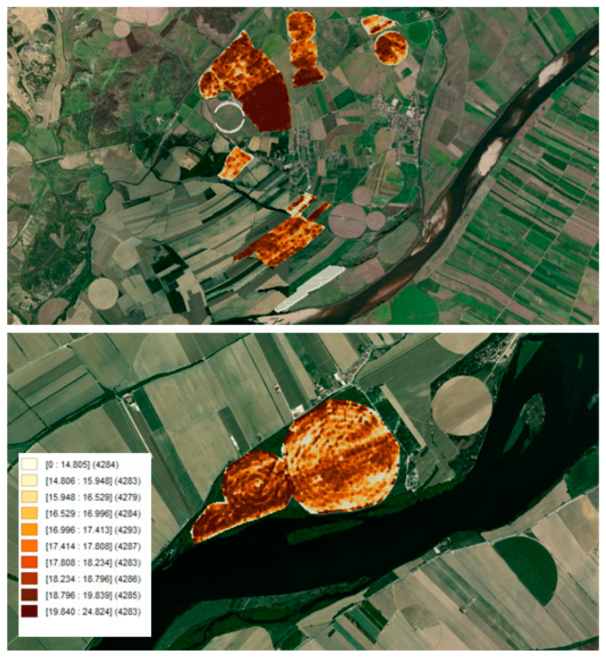
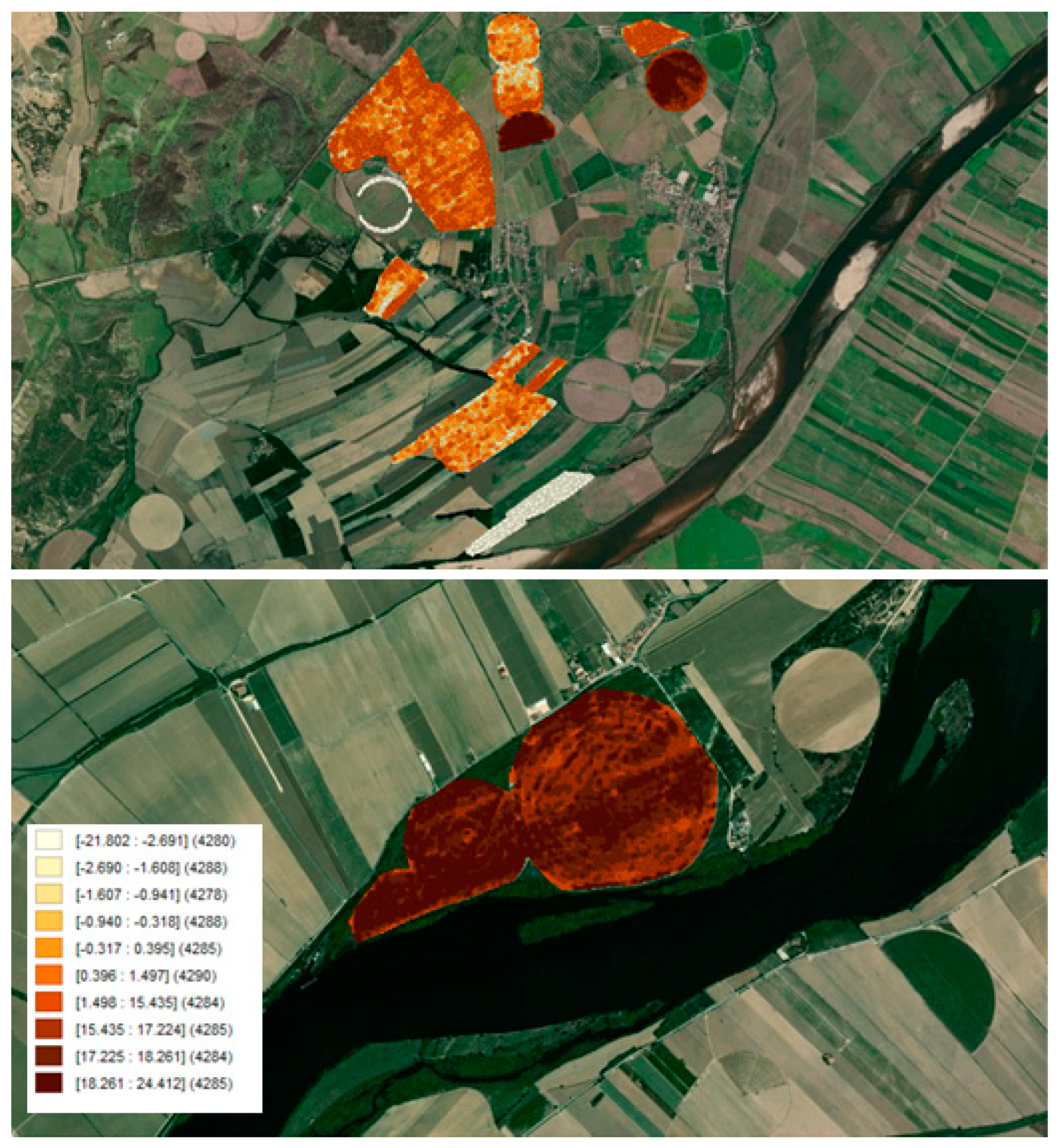
3.1. Data

The data used in this study were collected and provided by Portuguese firms using precision agriculture in maize cultivation. The maize exploitation in question is considered large, with approximately 542.5 hectares, in the years 2017 and 2018.

The companies have been developing efforts to collect as much data as possible in recent years. The entire maize farms were divided into 54,265 geo-referenced spatial units (ids). This unit definition originated from considering a 10-by-10-m square grid, which resulted in 100-square-meter spatial units. Although being part of more irregular parcels and sub-parcels, these smaller spatial units became the reference units for farm management and monitoring.

In order to assess management practices and options and their impact on maize yield, the analysis was carried out at the spatial unit level (id).

Concerning the data collection method, at the end of the season, the harvesters enter the farm and collect the maize. From these machines, with a width of 6 m, a shapefile is created, with the kilograms of the harvested maize in those spatial units. This data are then processed and filtered, and the errors due to the fragility of the machines are corrected.

For this study, the variable of interest is the average annual maize yield (y) measured in tons per hectare by id. This is determined by the dry weight of the harvested maize in a parcel/sub-parcel, indexed by the number of hectares of maize planted over time.

In Figure A1 and Figure A2 from Appendix A, we can see the spatial distribution of both yield (y) for 2018 and the variation in yield (Δy) for the same year. From Figure A1, it is possible to observe a great variability of yield in space. Combining the analyses of Figure A1 and Figure A2, a variety of situations combining the size of the level of maize yield with the size of its variation are also noticeable; that is, high level areas may show low increases of yield, medium or high, and low yield areas may be related to high increases from the previous year, medium or low.

The spatial dependence for both y and Δy can be assessed in Figure A3 and Figure A4 in the Appendix A. These figures plot, respectively, each variable against its spatial lagged value (obtained using a rook contiguity matrix). In particular, in Figure A3, it is possible to identify some spatial units that had zero or nearly zero production in 2018, despite being planted (facing a heavy decrease in production in comparison with the previous year’s campaign).

Apart from monitoring maize yield, climate data such as temperature in °C, precipitation in mm, relative humidity in percentage points, global solar radiation in W/m², and wind speed in km/h were collected daily for each sub-parcel with a 10-min frequency.

For the weather-related variables, the approach used in [28] was followed; being, consequently, those variables measured by maize development stage rather than by month, as is commonly seen in most agricultural econometric studies. The reason for this is the year-to-year variability of the crop and all factors associated with it. In this manner, in order to create variables by growth stages rather than by month, information was gathered on important dates in the maize life cycle, where four stages of maize growth were defined according to

Table 1. Definition of the maize growth stages.

Stage	Plant Activity	Starting Date	Ending Date
1	Emergence of the seedling from below the soil	Planting date (March/April/May)	Emergence date (April/May/June)
2	Early vegetative growth	Emergence date (April/May/June)	Flowering start date (June/July)
3	Flowering	Flowering start date (June/July)	Flowering end date (June/July/August)
4	Grain fill until maturity (harvest)	Flowering end date (June/July/August)	Harvest date (September)

Note: Both stages 1 and 3 only last about 15 and 10 days, respectively. Source: Own elaboration.

, following [28].

To obtain the weather data used in the model estimation, the following procedure was implemented. First, for each variable, the daily mean values were calculated. Then, with these daily values, the average of daily mean values (on the five climatic observed variables) was computed for each year (2017 and 2018) and each growth stage in Table 1. This high-frequency climate data provide, on one hand, a huge and rich dataset to measure climate effects on each stage, but, on the other hand, several variables that are highly correlated, inducing multicollinearity problems if all are included in linear regressions (naturally, temperature is correlated with all other climatic variables, such as relative humidity or global solar radiation among others). In this regard, more than one hundred climatic variables were preliminary analyzed and tested. The majority were dropped due to being insignificant for explaining the dependent variable.

Two other important sets of variables were collected: macronutrients and chemical treatments (herbicides and insecticides applied on different dates/stages for each sub-parcel).

To control for vegetation status, vegetative stress, and general crop health the normalized difference vegetation index (NDVI) of each spatial unit was assessed. NDVI is a satellite-derived vegetation index based in the soil vegetation cover, being the most widely used proxy for vegetation productivity. There is a strong relationship between the NDVI and crop yields. This index ranges between −1 and +1, where negative NDVI values represent non-vegetation surfaces, such as water bodies/masses, values close to zero refer to bare soils, and high values indicate strong vegetative cover. That is, the NDVI is a numerical indicator that analyzes the amount of live green vegetation in satellite images. The greener the observed vegetation is, the higher this index becomes. The information retrieved by the NDVI helps to better understand the behavior of crops during life cycle events and their response to natural or anthropogenic disturbances in agricultural ecosystems. See [33] for a commentary review on the use of NDVI.

In this study, during the crop campaign, 41 and 56 measures of NDVI in 2017 and 2018, respectively, were made for each sub-parcel. The first observed NDVI at an early stage was chosen to depict the potential maize seed vigor, given that in this early stage it is less prone to the interferences of other factors that affect yield productivity.

The effort and investments in data collection enabled defining several variables that were observed in 93% of the spatial units (50,547 spatial units) for the years of 2017 and 2018, in order to have a balanced panel.

For these variables, the same transformations and procedures performed on the climate variables were computed. In preliminary data analysis, most were not shown to be significant in explaining the behavior of maize production, and, as a result, were dropped from the estimation.

Table 2. Key variables for analysis.

Variable	Description
$y$	Maize yield (tons/ha)
$\mathsf{\Delta }y$	Annual change in Maize yield in 2018 (tons/ha)
$N$	Total Nitrogen (Kg/ha)
$P$	Total Phosphorus (Kg/ha)
$K$	Total Potassium (Kg/ha)
$I$	Total Irrigation (mm/ha)
$T\_S_i$	Average daily Temperature on Stage i (i = 1 to 4)
$Seeds$	Dummy variable equal to 1 if there was a change of Seeds used in previous year on the spatial unit, and 0 otherwise
$Treat$	Dummy variable equal to 1 if there was a change in Treatment (herbicides, insecticides) from the previous year on the spatial unit, and 0 otherwise
$Soil$	Dummy variable equal to 1 if the soil is clayey and equal to 0 otherwise
$ndvi$	First observed NDVI (early stage).

provides a summary of the final variables used in the empirical analysis of this article, after the preliminary selection procedure.

While Table 2 shows the key available variables,

Table 3. Descriptive statistics for 2018.

Variables	N	Minimum	Maximum	Mean	Std. Deviation
$y$	50,547	0	24.82	16.50	3.87
$\mathsf{\Delta }y$	50,547	−21.80	24.41	3.88	9.34
$N$	50,547	0	407.54	358.26	62.71
$P$	50,547	0	171.10	147.30	38.92
$K$	50,547	0	180.88	87.15	58.64
$I$	50,547	507.29	645.78	564.67	40.82
T_S1	50,547	13.40	18.79	16.77	1.12
T_S2	50,547	17.99	19.99	19.32	0.41
T_S3	50,547	20.12	24.70	20.55	0.64
T_S4	50,547	21.05	22.27	21.76	0.35
$ndvi$	50,547	0.14	0.36	0.20	0.05
$Soil$	50,547	0	1	0.50	0.50
$Treat$	50,547	0	1	0.30	0.46
$Seeds$	50,547	0	1	0.50	0.50

shows descriptive statistics for the above variables, which were used in the empirical model.

In a brief summary, Table 3 reveals that the average yield in 2018 was 16.5 tons/ha, and on average, there was an increase of 3.88 from the previous year, although with a great dispersion. Additionally, one can see that, while some spatial units had a production of zero, they all had some sort of nutrients applied and irrigation (the minimum values of N, P, and I were considerably above zero). Nitrogen was the nutrient used with the largest intensity, with an average around 360 Kg/ha, while the consumption of phosphorus and potassium was, on average, much lower, being, respectively, 147 and 87 Kg/ha. On the other hand, the use of potassium was the factor that varied the most within the farm spatial units.

As expected, the higher the maize growth stage, the higher the average temperature. The temperature variability was remarkedly higher in the first stage. The maximum average temperatures registered were below 25 degrees, not threatening crop productivity by heat stress.

Finally, the dummy variables are also worth noting, showing that 50% of the spatial units had a clayey soil (against 50% sandy soil), the treatment of herbicides/insecticides changed in 30% of the spatial units, and the type of seeds changed in 50% of the spatial units.

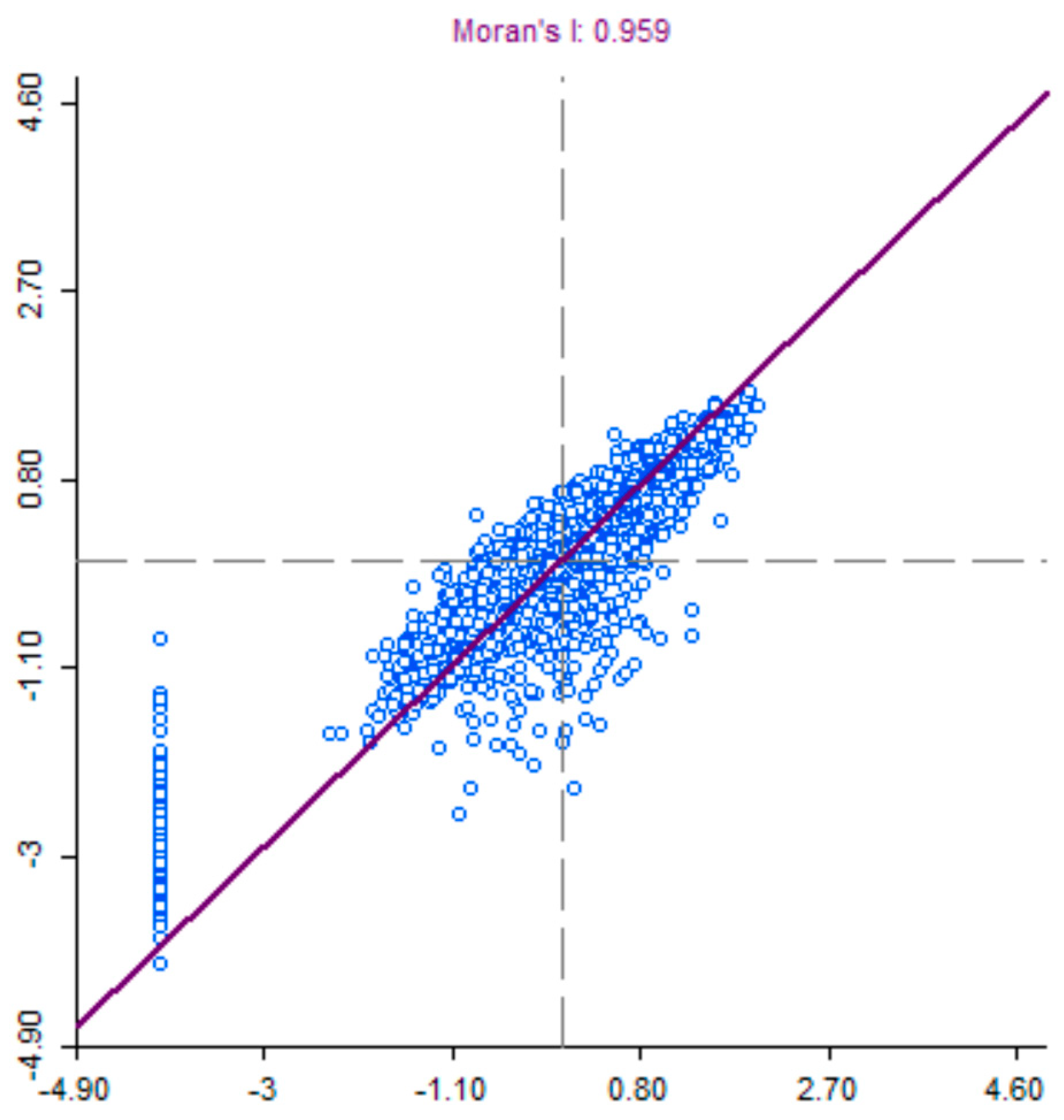
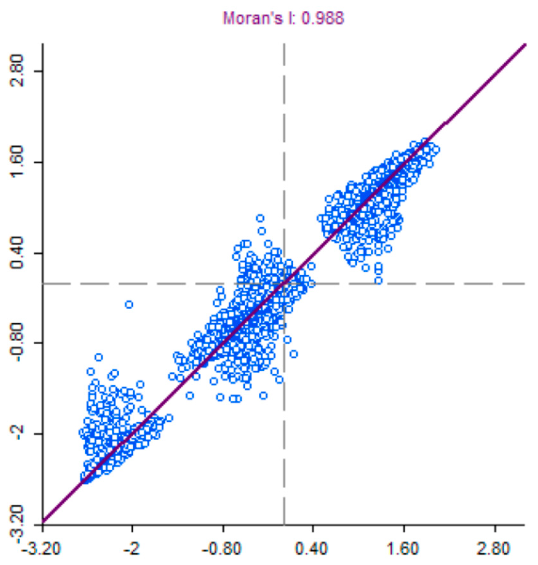
3.2. Methods and Results

As most geo-referenced variables are spatially autocorrelated and/or present spatial heterogeneity, spatial regression models are more appropriate than models that do not take spatial autocorrelation into account, as is the case of the linear model estimated by OLS. However, the OLS model is first fitted to obtain regression diagnostics for the spatial dependence of the residuals, with four statistical tests then being conducted to detect the presence of this spatial effect in linear models, such as the Moran test ([34]), the simple lagrange multiplier (LM Lag and LM Error) and their robust version (robust LM lag and robust LM error), as in [35,36]. The results can be seen in

Table 4. Statistical tests.

	Statistical Value	p-Value
Lagrange Multiplier (lag)	111,070.210	0.0000
Robust LM (lag)	108.396	0.0000
Lagrange Multiplier (error)	123,629.758	0.0000
Robust LM (error)	12,667.944	0.0000

, showing clear evidence of spatial dependence.

To control for spatial dependence, we followed Kelejian and Prucha’s approach [37], in which they advocated models that include both endogenous spatial interaction effects (by a spatial lagged dependent variable term) and spatial interaction effects among the error terms, leading to the so-called SARAR(1,1) model (spatial autoregressive of order 1 in the dependent variable and autoregressive of or-der 1 in the error term).

Although the data generated by the PA are sufficiently rich to allow the identification of many variables, it is natural, however, that some of the causes that influence the crop yield are not observed or even measurable, leading to the presence in the modelling process of unobserved heterogeneity. If the latter is correlated with the other variables in the model, then the usual estimation methods are inconsistent. However, with panel data it is possible to eliminate unobserved factors that are constant in time, i.e., factors specific to the spatial unit, using data transformations such as fixed effects or first differences. For example, in the data set used in this article, there are very few variables available that characterize the terrain attributes, and none regarding the topography of the spatial units. Given that we have a spatial panel data from 2 years (2017 and 2018), we can apply the mentioned transformations to remove these unobserved factors that are constant over time and, thus, eliminate the possible source of endogeneity that induces inconsistency in estimation. It is well known for panel linear models with only two periods of time that both transformations (fixed effects and first differences) should lead to the same results. Here, for sake of simplicity and convenience in estimation, first-differences transformation was chosen.

For the purpose of evaluating management practices, the main interest is to assess how farmer-controlled variables impact the variation in maize yield, such as choices about nutrient use, irrigation, and change in treatments and the type of seeds employed. Therefore, in the specification of the SARAR(1,1) model, those variables were included as explanatory variables. Climatic variables were included, as well as control variables. The squares of continuous variables were also considered to account for nonlinearities in model specification, given the complexity of the relation between agronomic inputs and crop yield and the absence of theoretical models to guide the empirical model specification.

Finally, the estimated model is

$$\begin{gathered} y_t=\rho W{y}_t+x_t{\mathsf{\beta }}_1+x_t^2{\mathsf{\beta }}_2+\theta ndv{i}_t+{\displaystyle \sum }_{j=1}^4{\gamma }_{j}T\_S{j}_t+{\delta }_{1}Seeds{ }_t+{\delta }_{2}Trea{t}_t+{\delta }_{3}SeedsTrea{t}_t+{\delta }_{4}Soil+\phi \\ +{\epsilon }_t with {\epsilon }_t=\lambda W{\epsilon }_t+u_t, t=2017, 2018 \end{gathered}$$

(1)

where W is the (N × N) spatial weigh matrix taken as known and non-stochastic; $y_t$ is a (N × 1) with the observations of maize yield in year t; $x_t$ is a (N × 4) matrix with the observations of the nutrients and irrigation in year t; ${\mathsf{\beta }}_j, j=1,2$ are (4 × 1) vectors of unknown coefficients; $ndv{i}_t$ is a (N × 1) vector with observations of the index NDVI in year t; $T\_S{j}_t$ j = 1,…, 4 are (N × 1) vectors with observations of temperature variables in year t; $Seed{s}_t$, $Trea{t}_t$, and $SeedsTrea{t}_t$ are (N × 1) vectors with observations in year t of the dummies Seeds, Treat, and their interaction, respectively; $Soil$ is a (N × 1) vector with observations of the dummy soil (does not change over time); $\theta$, ${\gamma }_j, j=1,\dots ,4$, ${\delta }_j, j=1,\dots ,4$, are unknown coefficients; $\phi$ is a (N × 1) vector of unobserved factors specific to the spatial unit (constant in time), possibly correlated with the other observable variables in the model; ${\epsilon }_t$ is the error term of the model in year t; $u_t$ is an idiosyncratic error, both (N × 1) vectors; and $\rho$ and $\lambda$ are the unknown spatial parameters. Note that to avoid unstable behavior, the constraints on the spatial parameters require that $\left|\rho \right|<1$ and $\left|\lambda \right|<1$. Here the spatial matrix W was calculated based on the contiguity queen criterion.

Applying the first differences transformation in Equation (1), all variables and factors that are constant in time are eliminated, leading to,

$$\begin{gathered} \mathsf{\Delta }{y}_t=\rho W\mathsf{\Delta }{y}_t+\mathsf{\Delta }{x}_t{\mathsf{\beta }}_1+\mathsf{\Delta }{x}_t^2{\mathsf{\beta }}_2+\theta \mathsf{\Delta }ndv{i}_t+{\displaystyle \sum }_{j=1}^4{\gamma }_j\mathsf{\Delta }T\_S{j}_t+{\delta }_1\mathsf{\Delta }Seeds{ }_t+{\delta }_2\mathsf{\Delta }Trea{t}_t+{\delta }_3\mathsf{\Delta }SeedsTrea{t}_t \\ +\mathsf{\Delta }{\epsilon }_t t=2018 \end{gathered}$$

(2)

where the operator $\mathsf{\Delta }$ gives the change in year 2018 from 2017 for each variable. The model in Equation (2) will be the one used for estimation purposes. However, for sake of interpretation of the coefficient estimates, it is more appropriate to use the untransformed model in Equation (1).

Besides considering the errors of Equation (2) as autocorrelated, the presence of heteroskedasticity is also acknowledge, following [37,38]. Estimation was performed with the GMM estimator of [38], since the first differenced data refers to a cross-section of one year. For the SARAR(1,1) Model in (2), a robust estimator of the covariance matrix in presence of both spatial heteroskedasticity and autocorrelation was considered, according to [38].

To interpret the effect of each of the x variables, ceteris paribus, one has to take into consideration the quadratic term. Therefore, the effect of changing x by one unit is given by ${\beta }_1+2{\beta }_{2}x$. This means that the effect is specific to the spatial unit and is a function of the level of x it consumes.

The results of the GMM estimation of model (2) with heteroskedasticity robust standard errors can be found on

Table 5. Spatially-weighted two-stage least squares with heteroskedasticity robust standard errors for the SARAR(1,1) model explaining the annual maize yield.

Variables	Coefficient	Std.Error	z-Statistic	Probability
constant	−3.26400	0.74712	−4.37	0.000
$\mathrm{W}y$	0.19722	0.01783	11.06	0.000
$N$	1.16329	0.08493	13.70	0.000
$N^2$	−0.00130	0.00012	−11.30	0.000
$P$	0.25149	0.04668	5.39	0.000
$P^2$	−0.00125	0.00020	−6.24	0.000
$K$	0.22823	0.00852	26.79	0.000
$K^2$	−0.00166	0.00006	−29.39	0.000
$I$	0.26508	0.01983	13.37	0.000
$I^2$	−0.00021	0.00001	−13.96	0.000
$ndvi$	12.80467	2.19045	5.85	0.000
$T\_S1$	−2.44472	0.14507	−16.85	0.000
$T\_S2$	−7.42977	0.55548	−13.38	0.000
$T\_S3$	−2.58341	0.13634	−18.95	0.000
$T\_S4$	−13.33222	0.59488	−22.41	0.000
$Seeds$	0.29953	0.22001	1.36	0.173
$Treat$	10.50346	0.85817	12.24	0.000
$Seeds Treat$	−9.51526	0.74883	−12.71	0.000
lambda	0.92361	0.00333	277.11	0.000
Pseudo R-squared = 0.9350.
n = 50,547

. For the GMM estimation, the additional instruments were Wz, z being all the independent variables.

Table 5 shows a very high value for the pseudo-R-squared, suggesting that the model provides a very good fit of the data. It also shows the effects on the annual variation of maize yield of several agronomic management variables, namely N (nitrogen), P (phosphorus), K (potassium), I (irrigation), Seeds (implying a change of the seeds used in previous year), and Treat (indicating a change in the treatment from previous year).

Table 5 shows that all variables were statistically significant at a 5% level, except for the dummy indicating change of seeds.

There are several important conclusions that can be drawn from Table 5.

First, one can notice that N, P, K, and I all show negative signs on their squared terms, meaning that these variables relate to the variation of maize yield as an inverted u-shape functional form. Consequently, the effect of these variables is not constant, and it changes sign from the turning point of the curve, which can be seen as the value of these variables that maximizes the yield. These values are included in

Table 6. Nutrients and irrigation values maximizing the average maize yield, and respective descriptive statistics.

Variable	Maximizer (M)	Minimum	Maximum	Mean	% Above M
$N$	447.04	0	407.54	358.26	0.%
$P$	100.84	0	171.10	147.30	84.8%
$K$	68.76	0	180.88	87.15	27.6%
$I$	645.90	507.29	645.78	564.67	0%

, together with some descriptive statistics.

Table 6 shows that the quantity of nitrogen (N) that maximizes the yield on average is higher than the maximum value observed, meaning that for all the spatial units increasing N will increase the average maize yield, but with diminishing returns.

The quantities of potassium (K) and phosphorus (P) that on average maximize the maize yield are below the mean observed in the sample, with a large percentage of spatial units (almost 85%) showing a use of phosphorus above the maximizer level, while this percentage drops significantly for potassium (28%), meaning that on average, for these units, increasing these nutrients will have a negative impact on average yield. This result may indicate that the farm is operating levels of P that are too high in a large percentage of spatial units.

Finally, the irrigation level that maximizes the yield in average is above the maximum irrigation registered in the sample. This means that, all the arable land is in a situation in which increasing units of I will have positive impacts on the average maize yield (at a diminishing rate).

Increasing the average temperature in each maize growth stage will, on average, decrease the crop yield, especially in the fourth stage, where one more degree of temperature will provoke an average decrease of 13 tons/ha, which is a very large impact. In the first and third stages, the impacts are smaller and similar, being around −2.5 tons/ha.

Regarding the NDVI, it presented a positive correlation with the yield variation, as expected.

Regarding the decisions about changing the seeds and changing the treatments, because of the interaction term, one may conclude that in those spatial units where treatment was not altered from the previous year, the change of the type of seed had no statistically significant effect on the maize yield, on average. The change of treatment in units where there was no change of the type of seed was successful because it led, on average, to an increase of the crop yield. The change of both the treatment and the type of seeds was also revealed to be successful, but with a much smaller impact than the latter.

4. Conclusions

This article illustrates how spatial econometric regression models can be useful to evaluate managerial agronomic decisions concerning crop production with PA data.

One important contribution of this work lies in the proposed model specification for the determinants of annual maize yield variation with the methodology used for estimation, given that the literature on this subject is scarce. This specification was a major challenge, given the enormous quantity of data typical from PA case studies, and relying on a preliminary computer-intensive data analysis. The final model was revealed to fit the data very well. It includes nonlinearities inducing heterogeneous effects on the mean of yield variation, which depend on the specific characteristics of the cultivated spatial units, being in line with the paradigm of PA. Moreover, it controls for spatial heterogeneity and spatial dependences recurring to spatial terms and spatial econometric techniques.

The results from this model suggested that decisions concerning the change in treatments (herbicides, insecticides) in the current year relative to those used in the previous year, incurred, on average, an increase of the maize crop yield, while when accompanied by a change of type of seed, this effect was attenuated.

Given that, on average, yield increased, the results show that the management practices for the current year were, in general, successful.

On one hand, the results seem to indicate that the management of nitrogen and irrigation have room for improvement, without harming, on average, the crop yield, where the levels observed in all spatial units were below the optimal level that maximized the yield.

Management of phosphorus and potassium should be balanced once a large percentage of the spatial units are still above the point where an increase of this nutrient has, on average (and ceteris paribus), a negative effect on crop yield.

The model also constitutes an important decision tool for management when the effect of each of the manageable input variables is not constant and equal for all spatial units, but depends on their level in each unit.

Finally, the model could be used to simulate the expected yield given expected values for the average temperature in each maize growth stage, and for nutrients, irrigation, and the decision about changing or not the type of seeds and treatment; with it being one more instrument that managers have at their disposal to define their agronomic decisions. More importantly, the analytical approach introduced in this work might provide a framework for managers to assess optimal levels for managed inputs for each specific farming context.

References

1. Oliver, M.A.; Bishop, T.F.; Marchant, B.P. (Eds.) Precision Agriculture for Sustainability and Environmental Protection; Routledge: Abingdon, UK, 2013. [Google Scholar]
2. Liaghat, S.; Balasundram, S.K. A review: The role of remote sensing in precision agriculture. Am. J. Agric. Biol. Sci. 2010, 5, 50–55. [Google Scholar] [CrossRef] [Green Version]
3. Tsouros, D.C.; Bibi, S.; Sarigiannidis, P.G. A review on UAV-based applications for precision agriculture. Information 2019, 10, 349. [Google Scholar] [CrossRef] [Green Version]
4. Bullock, D.S.; Bullock, D.G. From agronomic research to farm management guidelines: A primer on the economics of information and precision technology. Precis. Agric. 2000, 2, 71–101. [Google Scholar] [CrossRef]
5. Robertson, M.; Carberry, P.; Brennan, L. Economic benefits of variable rate technology: Case studies from Australian grain farms farms. Crop. Pasture Sci. 2009, 60, 799–807. [Google Scholar] [CrossRef]
6. Zhang, N.; Wang, M.; Wang, N. Precision agriculture—A worldwide overview. Comput. Electron. Agric. 2002, 36, 113–132. [Google Scholar] [CrossRef]
7. FAOSTAT. Crops and Livestock Products [Data Base]. 2021. Available online: http://www.fao.org/faostat/en/#data/QCL/visualize (accessed on 18 November 2021).
8. Chhetri, S.; Poudel, A.; Kandel, B.P.; Lamjung, N. Effect of Sowing Dates on Grain Yield and Other Agronomic Traits of Different Maize Inbred Lines. Int. J. Sci. Eng. Res. 2018, 9, 428–434. [Google Scholar]
9. Fang, J.; Su, Y. Effects of Soils and Irrigation Volume on Maize Yield, Irrigation Water Productivity, and Nitrogen Uptake. Sci. Rep. 2019, 9, 7740. [Google Scholar] [CrossRef] [PubMed]
10. Lobell, D.; Hammer, G.; McLean, G.; Messina, C.; Roberts, M.J.; Schlenker, W. The critical role of extreme heat for maize production in the United States. Nat. Clim. Chang. 2013, 3, 497–501. [Google Scholar] [CrossRef]
11. Schlenker, W.; Roberts, M.J. Nonlinear temperature effects indicate severe damages to U.S. crop yields under climate change. Proc. Natl. Acad. Sci. USA 2009, 106, 15594–15598. [Google Scholar] [CrossRef] [Green Version]
12. Chavas, J.-P.; Di Falco, S.; Adinolfi, F.; Capitanio, F. Weather effects and their long-term impact on the distribution of agricultural yields: Evidence from Italy. Eur. Rev. Agric. Econ. 2018, 46, 29–51. [Google Scholar] [CrossRef]
13. Liu, X.; Zhang, Y.; Han, W.; Tang, A.; Shen, J.; Cui, Z.; Vitousek, P.; Erisman, J.W.; Goulding, K.; Christie, P.; et al. Enhanced nitrogen deposition over China. Nature 2013, 494, 459–462. [Google Scholar] [CrossRef]
14. Ciampitti, I.A.; Vyn, T.J. Understanding Global and Historical Nutrient Use Efficiencies for Closing Maize Yield Gaps. Agron. J. 2014, 106, 2107–2117. [Google Scholar] [CrossRef] [Green Version]
15. Anselin, L.; Bongiovanni, R.; Lowenberg-DeBoer, J. A Spatial Econometric Approach to the Economics of Site-Specific Nitrogen Management in Corn Production. Am. J. Agric. Econ. 2004, 86, 675–687. [Google Scholar] [CrossRef]
16. Bongiovanni, R.; Lowenberg-DeBoer, J. Economics of nitrogen response variability over space and time: Results from the 1999–2001 field trials in Argentina. In Proceedings of the 6th International Conference on Precision Agriculture and Other Precision Resources Management, Minneapolis, MN, USA, 14–17 July 2002; pp. 1826–1841. [Google Scholar]
17. Lambert, D.M.; Lowenberg-DeBoer, J.; Malzer, G.L. Economic Analysis of Spatial-Temporal Patterns in Corn and Soybean Response to Nitrogen and Phosphorus. Agron. J. 2006, 98, 43–54. [Google Scholar] [CrossRef] [Green Version]
18. Liu, Y.; Swinton, S.M.; Miller, N.R. Is Site-Specific Yield Response Consistent over Time? Does It Pay? Am. J. Agric. Econ. 2006, 88, 471–483. [Google Scholar] [CrossRef]
19. Trevisan, R.G.; Bullock, D.S.; Martin, N.F. Spatial variability of crop responses to agronomic inputs in on-farm precision experimentation. Precis. Agric. 2021, 22, 342–363. [Google Scholar] [CrossRef]
20. Bockstael, N.E. Modeling Economics and Ecology: The Importance of a Spatial Perspective. Am. J. Agric. Econ. 1996, 78, 1168–1180. [Google Scholar] [CrossRef]
21. Lark, R.; Stafford, J.; Bolam, H. Limitations on the Spatial Resolution of Yield Mapping for Combinable Crops. J. Agric. Eng. Res. 1997, 66, 183–193. [Google Scholar] [CrossRef]
22. Kravchenko, A.N.; Bullock, D.G. Correlation of corn and soybean grain yield with topography and soil properties. Agron. J. 2000, 92, 75–83. [Google Scholar] [CrossRef]
23. Stone, J.R.; Gilliam, J.W.; Cassel, D.K.; Daniels, R.B.; Nelson, L.A.; Kleiss, H.J. Effect of Erosion and Landscape Position on the Productivity of Piedmont Soils. Soil Sci. Soc. Am. J. 1985, 49, 987–991. [Google Scholar] [CrossRef]
24. Kinoshita, R.; Rossiter, D.; van Es, H. Spatio-temporal analysis of yield and weather data for defining site-specific crop management zones. Precis. Agric. 2021, 22, 1952–1972. [Google Scholar] [CrossRef]
25. Afyuni, M.M.; Cassel, D.K.; Robarge, W.P. Effect of Landscape Position on Soil Water and Corn Silage Yield. Soil Sci. Soc. Am. J. 1993, 57, 1573–1580. [Google Scholar] [CrossRef]
26. Spomer, R.G.; Piest, R.F. Soil Productivity and Erosion of Iowa Loess Soils. Trans. ASAE 1982, 25, 1295–1299. [Google Scholar] [CrossRef]
27. Kaspar, T.C.; Colvin, T.S.; Jaynes, D.B.; Karlen, D.L.; James, D.E.; Meek, D.W.; Pulido, D.; Butler, H. Relationship Between Six Years of Corn Yields and Terrain Attributes. Precis. Agric. 2003, 4, 87–101. [Google Scholar] [CrossRef]
28. Dixon, B.L.; Hollinger, S.E.; Garcia, P.; Tirupattur, V. Estimating Corn Yield Response Models to Predict Impacts of Climate Change. J. Agric. Resour. Econ. 1994, 19, 58–68. [Google Scholar]
29. Huff, F.A.; Neill, J.C. Assessment of Effects and Predictability of Climate Fluctuations as Related to Agricultural Production; Illinois State Water Survey: Champaign, IL, USA, 1980. [Google Scholar]
30. Offutt, S.E.; Garcia, P.; Pinar, M. Technological Advance, Weather, and Crop Yield Behavior. North Central J. Agric. Econ. 1987, 9, 49–63. [Google Scholar] [CrossRef]
31. Daughtry, C.S.T.; Gallo, K.P.; Bauer, M.E. Spectral Estimates of Solar Radiation Intercepted by Corn Canopies 1. Agron. J. 1983, 75, 527–531. [Google Scholar] [CrossRef] [Green Version]
32. Stafford, J.V.; Bolam, H.C. Near-Ground and Aerial Radiometry Imaging for Assessing Spatial Variability in Crop Condition. In Proceedings of the Fourth International Conference on Precision Agriculture; Robert, P., Rust, R., Larson, W., Eds.; American Society of Agronomy, Crop Science Society of America, Soil Science Society of America: Madison, WI, USA, 1999; pp. 291–302. [Google Scholar] [CrossRef]
33. Huang, S.; Tang, L.; Hupy, J.P.; Wang, Y.; Shao, G. A commentary review on the use of normalized difference vegetation index (NDVI) in the era of popular remote sensing. J. For. Res. 2021, 32, 1–6. [Google Scholar] [CrossRef]
34. Kelejian, H.H.; Prucha, I.R. On the asymptotic distribution of the Moran I test statistic with applications. J. Econ. 2001, 104, 219–257. [Google Scholar] [CrossRef] [Green Version]
35. Anselin, L. Spatial Econometrics: Methods and Models; Kluwer Academic Publishers: Boston, MA, USA, 1988. [Google Scholar]
36. Anselin, L.; Bera, A.K.; Florax, R.; Yoon, M.J. Simple diagnostic tests for spatial dependence. Reg. Sci. Urban Econ. 1996, 26, 77–104. [Google Scholar] [CrossRef]
37. Kelejian, H.H.; Prucha, I.R. A Generalized Spatial Two-Stage Least Squares Procedure for Estimating a Spatial Autoregressive Model with Autoregressive Disturbances. J. Real Estate Financ. Econ. 1998, 17, 99–121. [Google Scholar] [CrossRef]
38. Kelejian, H.H.; Prucha, I.R. Specification and estimation of spatial autoregressive models with autoregressive and heteroskedastic disturbances. J. Econ. 2010, 157, 53–67. [Google Scholar] [CrossRef] [PubMed] [Green Version]