Rating Potential Land Use Taking Ecosystem Service into Account—How to Manage Trade-Offs

Abstract

Rating the potential land use for crop production and/or ranching is typically a process where production gains counterbalance environmental losses. Whereas the production gains are often easy to verify, the environmental losses may render visibility through the changes in the ecosystem service, such as water and habitat quality, carbon storage, etc., thus, leaving the decision maker with a multi-criteria problem. The present study demonstrates how partial-order methodology constitutes an advantageous tool for rating/ranking land use that takes trade-offs into account. It is demonstrated that not only the optimal choice of area, on an average basis, e.g., for crop production, is disclosed, but also the relative importance of the included indicators (production gains, ecosystem losses). A short introduction is given, applying data from a recent Chinese study looking for the optimal monoculture as a function of ecosystem tradeoffs. A more elaborate system applying data from the esgame was used, disclosing the most beneficial area for crop production and for ranching, as well as the relative indicators’ importance. The study further demonstrates that a single composite indicator obtained by simple aggregation of indicator values as a ranking tool may lead to a result where gains are optimized; however, this comes at the expense of the environment.

1. Introduction

Decisions about land use are often based on a single assumption, i.e., maximizing the yield, of crops or cattle-based products. However, agriculture or ranching may pose significant, typically negative influences on ecosystem services such as water and habitat quality, carbon storage, and hunting and foraging. Thus, in order to optimally rate or rank land use, it is necessary to consider the “costs” of the changes in the ecosystem services (ESs). Typically, we face positive production outcomes and gains on the ESs, on one hand, and negative impacts and losses on the other. Thus, optimizing the land use will be the result of a trade-off analysis considering the difference indicators [1].

A multi-criteria system (MIS) considers both the outcome of the production and the influence on the ESs. Very often, such systems are analyzed by a simple, e.g., arithmetic aggregation of the single indicators (criteria) to one composite indicator that allows a strict linear ordering of the objects studied. However, such analyses may be subject to erroneous results and, thus, decisions due to compensation effects [2], i.e., where one high value may be compensated by other rather low values, without knowing the actual influence or importance of the single indicators. Hence, multi-criteria decision analyses (MCDAs) may advantageously be brought into play. MCDAs have previously been used in the study of ecosystem services [3,4,5,6,7,8]. These studies review or apply a variety of MCDA methods for trade-off analyses of ecosystem services. A joint trend is that the weights are introduced in an attempt to generate a composite indicator by aggregation (see, e.g., [7,8]) or comparing indicators pairwise, as proposed by Lee and Launtenbach [3]. In none of these studies do the applied methods bring all indicators simultaneously into play without pretreatment, as, e.g., weighted aggregation. Hence, MCDAtaking all indicators into account simultaneously may advantageously be brought into play.

To remedy this and to further add to the toolbox, the present study introduces a partial order methodology (cf., e.g., [9,10,11,12,13,14,15,16,17] as a method to analyze MISs, and it focuses on the tradeoffs between production outcome and changes in ecosystem services.

Partial ordering is an advantageous methodology for such studies as it considers all features (indicators) simultaneously without any pre-assumptions or pretreatments such as aggregation. As such, the analyses avoid potential problems such as compensation effects [2]. Thus, the influence/importance of the single indicators is immediately disclosed by partial order analyses, which may constitute important information for decision makers as they here suggested, e.g., that resources should be allocated for improvements of the system.

The overall objective of the study is to provide a simple MCDA, that is, a partial ordering methodology to analyze MISs, in this case trade-off issues in land use, by taking ecosystem services into account. The partial order methodology is briefly described in Section 2; however, references to the available literature for a deeper theoretical background and understanding of the techniques are provided. Hence, the analyses of trade-off issues will initially be illustrated by a simple exemplary case based on data from a recent Chinese study [18] (Section 3.1), followed by a more elaborate system applying data from the trade-off game [19,20] (Section 3.2 and Section 3.3). Finally, Section 4 provides conclusions and some outlooks on how the methodology may be applied.

Why Partial Ordering

When an MIS is to be evaluated, multivariate statistical methods such as correlation or regression analyses and clustering techniques are of primary interest. In some studies, only a regression analysis is considered as a method for an evaluation of an MIS [21]. However, regression analyses need a model concept, e.g., whether a linear model is appropriate or not or whether a nonlinear fitting model appears as a more appropriate choice. To some degree, this is also the case for principal component analyses. In the case of cluster analysis, the answer needs a few more remarks. In addition to the technical problem of how to define distances among groups of objects (cf. [22,23]), cluster analyses have no evaluative background, as the clustering is a result of distance measures. Nevertheless, the method appears attractive, and attempts to infer a posteriori ranking perspectives have been reported (cf., e.g., [24]). Partial order methods have their own disadvantages, such as the loss of any metric. However, the evaluative aspect is its main advantage. The comparison of the objects of interest is carried out simultaneously for all indicators, without the need for any prior aggregation (details below). In summary, the application of partial order methodology, at least as an interim process before other tools will be applied, is emphasized.

Although partial ordering is a relatively new method, the methodology has been demonstrated to be valuable in a wide variety of disciplines (cf., e.g., [10,25,26,27,28,29,30,31,32,33,34])

2. Methodology

2.1. Partial Ordering—The Basics

The basis for partial ordering is the relation among the objects to be ordered. Formally, the only mathematical term in this context is the “≤” relation (cf., e.g., [9,10,11,12,13,14,15,16,17]). The role of this relation is fixed up by following axioms [10]:

Axiom 1: Reflexivity:   x ∈ X: x ≤ x

(1)

Axiom 2: Anti-symmetry:  x ≤ y, y ≤ x implies y = x

(2)

Axiom 3: Transitivity:  x ≤ y and y ≤ z implies x ≤ z

(3)

Reflexivity means that a given object can be compared with itself.

Anti-symmetry means that if both comparisons are valid, i.e., y is better than x and at the same time, x is better than y, then this axiom demands that x is identical with y. Instead, we accept equivalences.

Transitivity means that if the objects are characterized by properties which are at least ordinal scaled, then any measurable quantity such as height, length, price, etc. implies transitivity.

Hence, the “≤” relation is the basis for a comparison of objects and constitutes a graph, the so-called Hasse diagram (see below). Two objects relate to each other, i.e., are comparable if and only if the relation x ≤ y holds. Since a given object, x, is characterized by the a set of indicators r_j(x), j = 1, …, m, it can be compared to another object y, characterized by an identical set of indicators r_j(y), if

r_i(x) ≤ r_i(y) for all i = 1, …, m

(4)

which requires that at least one indicator value of object x must be lower and the remaining lower or at least equal to those of object y if a comparison should be established. If Equation (2) does not hold, the two objects will be incomparable (notation: y ǁ x). The two objects with all indicators that have identical values and are equal are denoted equivalent (notation: x ~ y); in ranking terms, this means that they will have the same.

Concepts of Partial Ordering

Given a partial order some concepts are of importance. Let us look at two objects, x and y, in the MIS.

• Max(MIS): the set of objects of the MIS, where no other object y can be found with y > x. This is the set of maximal objects of a partially ordered set (poset). If x is the only maximal object, it is called the “greatest” object;
• Min(MIS): the set of objects of the MIS, where no other object y can be found with y < x. This is the set of minimal objects of a poset. If x is the only minimal object, x is called the “least” object;
• Iso(MIS): the set of elements of the MIS that at the same time are elements of Max(MIS) and Min(MIS). Such objects are called isolated objects. Within the context of a MIS the data values leading to objects that are not compared to any other object. These elements may be of special interest;
• Chain: A subset of the MIS, where each object is mutually comparable with others;
• Antichain: A subset the MIS, where each object is mutually incomparable with others;
• Level: The subset of the MIS, where all objects have the same rank.

The construction of the system of levels taken from a poset is of special importance. Algorithmically, it is not the best way to follow the definition but to define an iterative procedure, as explained in Bruggemann and Patil [10]. By levels a weak order is defined. A weak order is an order, where equivalences are accepted. For example, the sequence a < b = b = c < d < e = f is not an order, because there are equivalences, but it is a weak order. From a statistical point of view the fact of equivalences is considered as disadvantageous, because objects are insufficiently separated. Within the context of partial order, the level structure is often a first attempt to find a weak order for a given objects. Note, if the MIS is a chain, i.e., all objects of the MIS are mutually comparable, then each level consists of only one object and then the level structure defines an order.

For a deeper theoretical explanation of the methodology the above-mentioned references should be consulted.

2.2. The Hasse Diagram

Equation (1) is the basis for the Hasse diagram technique (HDT) [10,25]. Hasse diagrams are visual representation of the partial order. In the Hasse diagram comparable objects are connected by a sequence of lines [10,11,25,30,31]. Thus, sets of comparable objects, i.e., fulfilling Equation (1) are called chains that in the diagram are connected with lines, whereas sets of mutually incomparable objects, i.e., not fulfilling Equation (1) are called antichains.

In the diagram the single objects are positioned in levels, typically arranged from low to high (bottom to top in the diagram). A general rule is that objects are located a high in the diagram as possible. Thus, isolated objects, i.e., objects that are not comparable to any other objects, will by default be placed at the top level of the diagram. In the case of equivalent objects only one representative for each of the equivalent classes will be shown in the diagram.

The module mHDCl7_1 of the PyHasse software (vide infra) was used for the basic partial ordering calculations and the associated construction of the Hasse diagrams.

The Orientation

It is important to make sure that the orientation of the single indicators is identical, e.g., that high values correspond to “good”, whereas low values correspond to “bad”. In practice, this is carried out by multiplying indicator values by −1 in case where high and low values correspond to “bad” and “good”, respectively (cf. Section 2.5). In the present study, the highest located object will be assigned rank 1 indicating the “best”.

2.3. Average Ranking

Looking at the Hasse diagram, the level structure constitutes a first approximation to ordering/ranking. However, as all objects in a level automatically will be assigned identical ranks such an ordering will obviously cause many tied orders. Obviously, it is desirable with a degree of tiednes being as low as possible. Hence, ultimately a linear ordering of the single objects is desirable. However, when incomparable objects are included in the study, obviously this is not obtainable. Partial order methodology provides a weak order, where tied orders are not excluded by calculating the average order of the single objects as, e.g., described by Bruggemann and Carlsen [32], Bruggemann and Annoni [33] and Carlsen and Bruggemann [16].

This method is mainly a combinatorial exercise, and one is confronted with computational difficulties if the MIS is a large set (more than 50 objects). This difficulty triggered many mathematical approaches how to circumvent the computational problems. A relatively famous method is the Monte Carlo Markov chain method proposed by Bubley and Dyer [29]. A “quick and dirty” method is the concept of local partial order, proposed by Bruggemann et al. [34], where the basic idea is to check the order theoretical environment of each single object of the MIS. The crucial question is, how large must the environment be selected to obtain reliable results. Depending on the selection of the environment different Local Partial Order Models (LPOM) arises. In the present study, the LPOMext is selected, where not only the chains, encompassing object x are considered but also its incomparable objects U(x): = {y ∈ X, with y ‖ x} (for details, see [32]).

The LPOM methods were compared with the results of an exact method, based on lattice theory [35,36] with surprisingly good results. However, the method by lattice theory fails when the MIS is large.

The average rankings were calculated applying the LPOMext9_1 [32] module of the PyHasse software (vide infra).

2.4. Sensitivity-Indicator Importance

A Hasse diagram has a certain structure (cf. Section 3.2). Thus, levels, isolated objects, chains, etc., constitute the “structure” of the diagram and, thus, the partial order. The structure of a Hasse diagram, in turn, is important for an elucidation of the data and their interpretation. The obvious question is, how the single indicators would affect the structure.

The relative importance of the single indicators in play can be determined through a sensitivity analysis [37]. The basic idea is to construct partial ordered sets (posets) excluding the single indicators one at the time. Subsequently, the distances from these posets to the original poset are determined. The indicator, whose elimination from the original poset leads to the maximal distance to the original one, in other words causing the highest degree of changes in the Hasse diagram is important for the structure of the original partial order [16].

The sensitivity values were calculated by the sensitivity24_5 module of the PyHasse software (vide infra).

2.5. Indicators

The rating of land use, taking the ecosystem service into account, is based on an indicator describing the gains/outcomes by the agricultural or ranching activities and 4 indicators describing the influence on four ecosystem services, i.e., carbon storage, habitat and water quality and hunting and foraging, respectively (Table 1). Two sets of indicators, for agriculture and ranching, respectively, are used.

Table 1. Indicators applied.

Indicator	Notation	Explanation
Production	crop_ag/past_ps	Agriculture/Ranching
Ecosystem service	agcarb/pscarb	Carbon storage (Agriculture/Ranching)
Ecosystem service	aghq/pshq	Habitat Quality (Agriculture/Ranching)
Ecosystem service	agwq/pswq	Water Quality (Agriculture/Ranching)
Ecosystem service	agrec/psrec	Hunting and Foraging (Agriculture/Ranching)

2.6. Data

2.6.1. The Exemplary Case

The data applied for the Chinese study was adopted directly from the paper by Zou et al. [18] summarizing the relative ecosystem services (Table 2).

Table 2. The relative ecosystem services (RES) of the seven monoculture patterns.

RES	Provisioning	Regulating	Supporting	Cultural
Corn	0.021	0.052	0.154	0.252
Marigold	0.052	0.23	0.141	0.504
Orange	0.025	0.587	0.473	0.607
Pear	0.144	0.576	0.586	0.607
Peach	0.038	0.881	0.846	0.607
Apple	0.169	0.872	0.811	0.814
Pomegranate	0.955	0.508	0.678	0.814

2.6.2. The Esgame

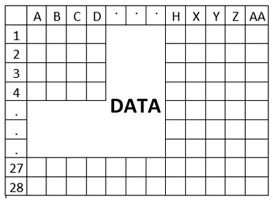
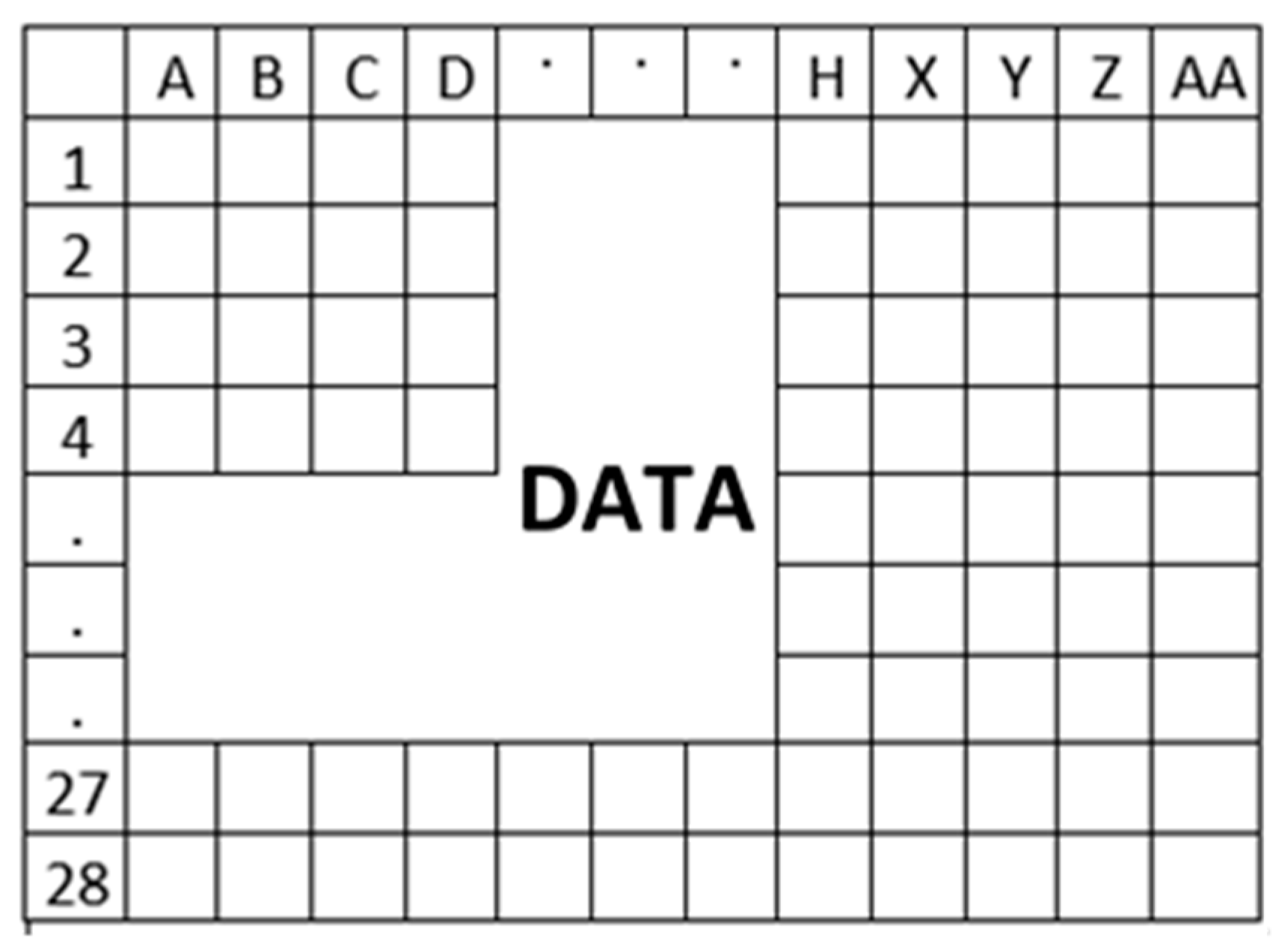
The data for the esgame study was obtain from Lacayo [19] and esgame [20]. The raw data [19] were transformed to fit the esgame [20], i.e., a 27 × 28 grid of square pieces of land. For each of these grid points values of the above-mentioned indicators are calculated. The unit of the indicator values is identical for all indicators. In total 5 indicators (columns) and 756 grid points (rows) constitute the MIS (Figure 1). Two separate MIS were obtained: one based on agriculture, i.e., crop production and one based on ranching, respectively. The color coding disclosing the distribution of indicator values can be found at the esgame web site [20]. Due to the actual size of these two MIS the data are not included in the present paper but can be obtained from the author upon request.

Figure 1. The area being investigated in 756 grid points.

As the production, i.e., crop production or ranching, in the esgame is considered to have a negative influence on the four ESs, the ESs indicators all have negative values in the MIS. Thus, for all indicators the term the higher the better prevails.

2.7. Software

All partial order analyses were carried out using the PyHasse software [26]. PyHasse is programmed using the interpreter language Python (version 2.6). Today, the software package contains more than one hundred specialized modules and is available upon request from the developer, R. Bruggemann (brg_home@web.de).

3. Results and Discussion

3.1. An Exemplary Case

To illustrate the partial ordering methodology, data from a recent Chinese study on trade-off analysis of ecosystem service [18] serve as an exemplary case. Thus, Zou et al. (2020) study the performance of ecosystem services (ESs), provisioning, regulating, supporting and cultural (cf. [18], Table 2) for seven typical monoculture patterns: corn, marigold, orange, pear, peach, apple, and pomegranate.

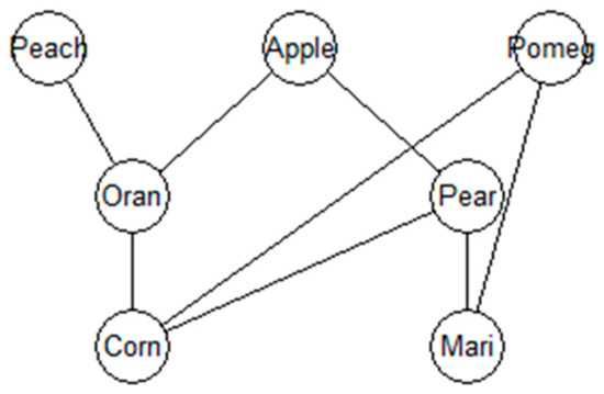
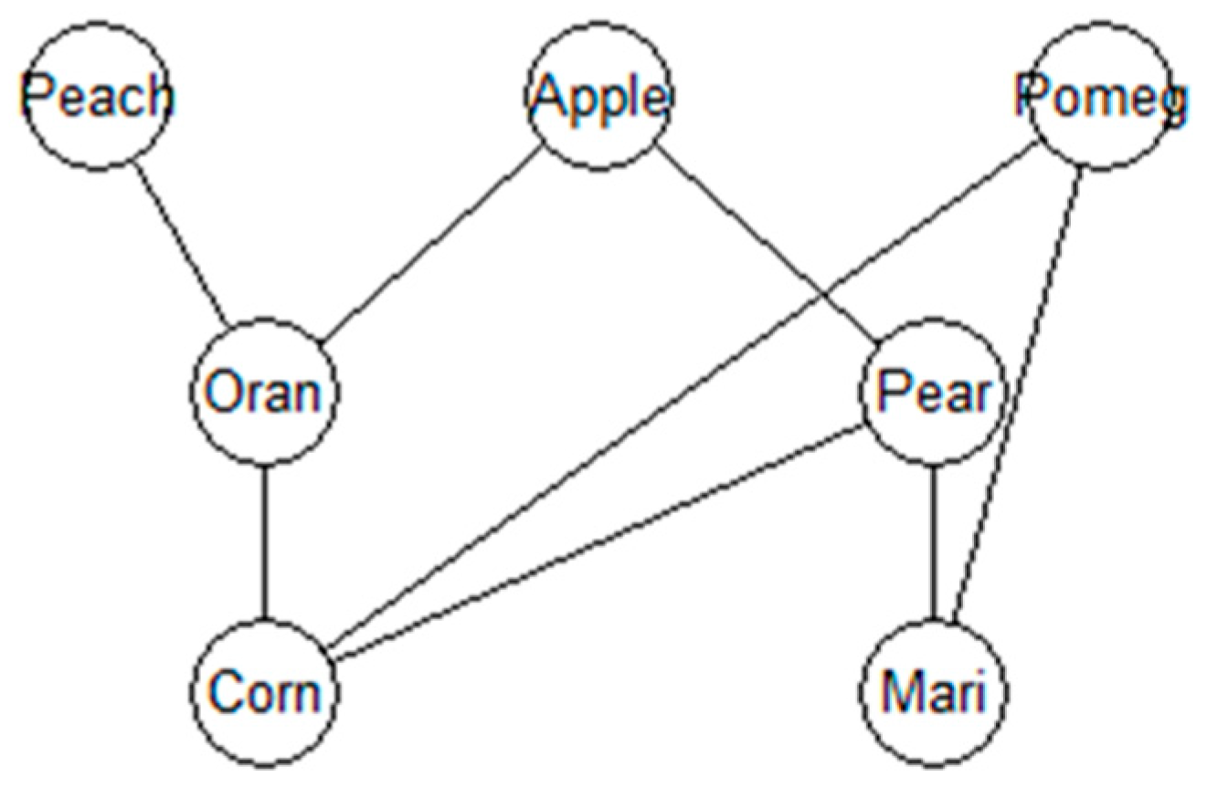
Based on the values given in Table 2, Zou et al. [18] draw a series of conclusions on the ecosystem services in the different monoculture patterns. However, they were not able to draw a final conclusion. Applying partial ordering, on the other hand, it is possible to obtain a more comprehensive picture, bringing all 4 ESs (the indicators) simultaneously into play. In Figure 2, the resulting Hasse diagram is shown.

Figure 2. Hasse diagram visualizing the partial ordering of the seven monoculture pattens (cf. Zou et al. [18]).

It is immediately noted that peach, apple, and pomegranate appear at the top level of the diagram and as such is expected to be the most beneficial cultures in agreement with Zoe et al. [18]. Calculating the average ranking an even more decisive picture of the seven monocultures developed. Hence, we found apple from an ES point of view constitutes on an overall average basis as the preferable monoculture, the rating of the seven monocultures according to their qualifications to be Apple > Peach > Pomegranate > Pear > Orange > Marigold > Corn.

Looking at the relative importance of the single ESs it was disclosed that provisioning (0.500) > regulating (0.375), supporting (0.125) and cultural (0.000), i.e., that the cultural ES does not influence the partial ordering of the seven monoculture pattens, which with reference to the paper by Zou et al. [18] may not be surprising as this ES summarizes the “cost according to the equivalent education level of training” (cf. [18], Supplementary File S1).

3.2. The Esgame-Agriculture

As mentioned above, we are looking at a larger piece of land that has been divided into 27 × 28 = 756 square grid points (cf. Figure 1). Formally, the dimension of the land and grids are arbitrary. However, for clarity the single grids could be a 1000 × 1000 = 1,000,000 m², i.e., 100 hectar, which roughly corresponds to an average UK farm [38]. Each of the grid points are characterized by the 5 indicators crop_ag, agcarb, aghq, agwq and agrec (cf. Table 1). Quite a few of the grid points appear to be equivalent leaving 470 equivalent classes (cf. Section 2.2). Some of them are trivial classes, i.e., containing only one single grid point (called trivial equivalent classes), while other contain quite a few. Thus, the major non-trivial equivalent class contains all grid points where all indicator values equal zero. This class contains 274 objects. Further, 2 equivalent classes with 3 object and 8 with 2 objects, respectively, are present. The remaining 459 grid points are unique, i.e., trivial equivalent classes.

Overall, the 756 grid points can be divided into three main groups: (a) a group where all indicator values equal zero, meaning no production and thus no influence on the ESs, (b) a group where the combined data reflect that although we have a certain production the positive outcome is more than compensated by the negative influence on the ESs and (c) a group where the outcome of the production is higher than the negative impacts on the ESs. Obviously, the eventually preferred grid point is to be found within group c.

In contrast to the above exemplary case (Section 3.1) it has no meaning to graphically to visualize the Hasse diagram based on the agriculture MIS. Obviously, the information content of a Hasse diagram with 470 objects distributed over 12 levels is rather limited. Thus, in Table 3 a tabular version of the diagram is given.

Table 3. Tabular version of the Hasse diagram corresponding to the agriculture grid. The naming of the single grid point corresponds to their location (cf. Figure 1).

Level	No of Grid Points	Grid Point (Equivalent Classes)
12	31	A1 C23 H20 I10 I11 I12 J10 J11 J17 K27 L8 L13 L27 M7 M9 M13 M26 N17 N21 N26 N27 S24 S26 S27 T17 T23 T24 T26 T27 U24 Y15
11	55	A21 B22 B23 D12 D15 E10 E11 E22 F10 F11 F22 G21 I17 I19 J20 J21 K7 K10 K20 K26 L7 L9 L12 L26 M10 M11 M20 M27 N18 N22 O17 O23 P14 P26 Q14 Q15 Q24 R2 R3 R15 R28 U8 U9 U17 V3 V7 W4 W6 X15 X22 Y9 Y10 Y14 Y16 Y18
10	70	D16 E12 E15 F12 F23 G22 H14 H19 I13 I18 J18 J22 J23 K6 K8 K11 K19 L4 L5 L6 L19 L20 M2 M6 M8 M12 M18 N2 N7 N16 N20 O2 O3 O6 O7 O9 O18 O22 O24 P6 P15 P23 P24 Q2 Q28 R14 R27 S12 S14 S17 S28 T12 T14 T18 U14 U16 U18 U21 U22 U23 V4 V22 W22 X9 X10 X16 X17 Y19 Z10 Z14
9	64	A18 A20 A22 B18 B19 C22 E13 E16 F13 G10 H12 H17 H18 H21 J16 J19 K9 K13 K16 K22 K23 K24 L3 L10 L11 L25 M17 M19 N10 N12 N13 N14 O27 P5 P25 Q13 Q23 R4 R16 R24 S2 S3 S11 S13 S23 T8 T11 T15 T16 T21 T22 U7 U15 V6 V14 V23 W3 W12 X11 X12 Y11 Y17 Y21 Z9
8	57	D20 D22 D23 E14 E23 G19 G20 H11 H13 I20 J12 K17 K21 K25 L2 M14 M21 N3 N4 N15 N23 O5 O10 O14 O16 O26 P2 P7 P27 Q11 Q12 Q16 Q25 R10 R23 S9 S10 S16 S25 T3 T6 T13 T19 U4 U10 V1 V11 V12 V13 W2 W8 W13 X14 Y12 Y20 AA10 AA14
7	64	A17 A19 B17 B20 G12 G16 G17 H10 J13 K12 K15 K18 L16 L17 L18 L21 M3 M4 M25 N8 N9 N11 N19 N24 O4 O13 O25 P3 P4 P8 P9 P10 P12 P13 P16 P28 Q3 Q5 Q7 Q10 R5 R22 R26 S15 T1 T9 U1 U12 U13 U19 V5 V9 V10 V21 W7 W9 W11 W14 W17 X13 Y13 Z13 AA11 AA13
6	56	B21 C17 D19 E18 E20 F17 F19 G11 G15 G18 I16 L22 L24 M16 M22 M24 N6 N25 O8 O11 O20 O21 P11 P22 Q4 Q6 Q9 Q17 Q18 Q22 R6 R7 R11 R17 R18 S4 S5 S6 S22 T2 T5 T7 T25 U3 U6 U11 V2 V15 V18 V19 W10 W15 X18 X21 Z11 AA12
5	35	C18 C20 D17 D18 E17 E19 F18 F21 G14 H16 I14 L14 M23 O12 O19 Q8 Q21 Q27 R13 R19 R21 S7 S8 S18 S19 T4 T10 U2 V8 V16 V17 W16 W19 X19 X20
4	23	C19 C21 D21 E21 F16 F20 G13 H15 K14 L15 L23 M5 M15 P17 Q19 Q20 Q26 R9 R12 R20 U5 W18 W20
3	10	F14 I15 J14 J15 N5 P18 P19 P21 R8 W21
2	4	S20 S21 T20 V20
1	1	U20

Obviously, the above Hasse diagram only gives rather limited information concerning the actual ranking of the single grid points, as all objects in a given level are associated with the same rank. For a deeper insight into the mutual ranking of the grid points, the average ranking (cf. Section 2.3) is calculated. The top 10 grid points, i.e., the points that, on an average basis, appear as the most beneficial for agriculture (crop production) were found to be I11 > J11 > J10 > L13 > L8 > M13 > I12 > Y15 > N17 > K10, respectively (for notation cf. Figure 1). It can be noted that the top 9 grid points are found in level 12 of the Hasse diagram whereas the rank 10 grid point, K10, is located at level 11.

It is interesting to note that the grid point I11 on an average basis appears as the preferable, with an overall sum of the indicators equal to 675 count units. However, the maximum sum, which equals 750 count units, is, however, found for grid point M13, the value being obtain by a simple arithmetic aggregation of the five indicators. M13 is, on an average basis, found at rank 6. To explain why M13 should not be regarded as the top-ranked grid point, it is necessary to look at the indicator values for the two grid points (Table 4).

Table 4. Indicator values of the top ranked grid point based on an average ranking (I11) and an aggregation process (M13).

Grid Point	crop_ag	agcarb	aghq	agwq	agrec	SUM
I11	1050	−100	−150	−50	−75	675
M13	1500	−200	−300	−150	−100	750

First, the difference in the ranking methods should be emphasized. The top ranking of I11 is based on an average ranking where all five indicators are considered, whereas in the case of M13 the ranking is based on an aggregation, here a simple arithmetic sum, of the five indicators; thus, small values are compensated by large values.

A closer look at the figures leads to a clear explanation of the differences between I11 and M13, thus pointing at I11 as the optimal choice and partial ordering as a superior methodology. The problems associated with compensation effects when applying composite indicators has been discussed previously in several of papers dealing with partial ordering (cf., e.g., [2,10,11,12,13,14]).

It is clear (Table 4) that the outcome, crop_ag, of M13 is approx. 43% higher than for I11. Thus, a first look indicates that M13 is a more optimal choice that I11. However, focusing on the environmental impact, as visualized through the values of the five ES indicators, it immediate becomes obvious that the environmental impact in the I11 grid point is significantly lower that found for M13. Hence, in the latter case the high outcome overshadows, compensates the higher environmental impact. This leaves the decision maker with an obvious and highly relevant question: are we willing to sacrifice the environment in favor of a higher outcome from production?

Indicator Importance

In addition to the valuable information disclosing the grid point that on an average basis constitutes the optimal choice for the agricultural crop production, it appears to be of interest to verify the relative importance of the single indicators. This information is obviously of interest in order to clarify which of the ESs that play the most important role in the overall rating, thus, suggesting, e.g., which area where possible resources should be allocated in order to improve the environmental state of the area and possibly leave some additional space for a higher production rate. Such information is not available applying the composite indicator as ranking measure since the information is hided through the aggregation process.

The relative importance of the five indicators included in the study is estimated through a sensitivity analysis (cf. Section 2.4). The relative importance of the five indicators were found to be crop_ag (0.833) > aghq (0.093) > agwq (0.043) > agrec (0.021) > agcarb (0.009). It may not be surprising that the most important indicator is the actual production indicator crop_ag that account for close to 85%. For the ESs the result suggests that the most important ES is the habitat quality followed by the water quality, which, taking the crop production into account again may not be surprising. In the case of water, probably the water is used for irrigation that will obviously use water but not necessarily have significant impact on the quality, whereas clearing land for crop production may have significant impact on the habitat quality.

3.3. The Esgame-Ranching

The second part of the esgame is focused on production by ranching [20]. Obviously, the impact on the ecosystem services is different from those from agriculture by crop production. However, the overall picture is quite similar. Thus, we deal with 463 equivalence classes of which the by far biggest group is the one where all indicator values equal zero. As in the case described above, the resulting Hasse diagram features 12 level with 2, 11, 15, 36, 43, 44, 47, 49, 65, 70, 53 and 28 objects in the levels 1 to 12, respectively. The top 10 grid point based on an average ranking are L13 > E11 > P24 > O24 > P23 > M13 > X12 > R15 > F11 > Q23.

Hence, average ranking reveals the grid L13 as the most advantageous place for ranching, although based on the simple aggregation of the indicator values the Q23 grind point, which on an average basis has been assigned the rank 10, has the highest rank. In Table 5, the indicator values for the grid points L13 and Q23 are given.

Table 5. Indicator values of the top ranked grid point based on an average ranking (L13) and an aggregation process (Q23).

Grid Point	past_ps	pscarb	pshq	pswq	psrec
L13	800	−100	−125	−25	0
Q23	950	−100	−125	−50	−25

As in the agriculture example above, also here is seen that the maximum outcome is associated with grid point Q23. However, the increased outcome has been paid by an increased impact on the environment, i.e., an increased negative impact on the water quality and the hunting and foraging (cf. Table 1); thus, the same question as above arises: are we willing to pay for the increased outcome by an increased environmental degradation?

Turning to the indicator importance again, a picture close to that described above for crop productions is found, the relative importance being past_ps (0.810) > pshq (0.096) > pswq (0.057) > pscarb (0.023) > psrec (0.015). Again, the actual production indicator, past_ps, appears as the most important, not surprisingly followed by habit and water quality.

4. Conclusions and Outlook

The general applicability of partial order methodology for studying multi-indicator systems, as here the rating/ranking of land use has been elucidated based on a simple exemplary toy example adopted from a recent Chinese study and further by a significantly elaborate system, the data being taken from a recent game to study trade-off issues in agriculture and ranching. It has been demonstrated that a simple arithmetic aggregation of indicator values may well lead to the highest outcome, e.g., through crop production or ranching; this may not be consistent with focusing on the lowest negative impact on the ecosystem services. Thus, taking all indicators into account simultaneously, i.e., apart from the production outcome, also considering the impact on the involved ecosystem services such as water and habitat quality, carbon storage and Hunting and Foraging, a different picture develops. It is obvious that the higher production outcome apparently is overshadowed by an increased, and thus unwanted, deterioration of the ecosystem services. This obviously calls for an answer to the unavoidable question: do we want to accept a higher production outcome on the expense of the environment, here the ecosystem services? In other words, partial ordering leaves us with a clear picture of the relative influence of the single indicators, which in turn offers the regulators an efficient tool to focus on the specific targets that on an overall basis will improve the system at the most. Further, it is clear that such valuable information would not be provided when applying a composite indicator due to compensation effects. Hence, it is clear that aggregation may well lead to erroneous or, in the best case, questionable results [2].

The present study further demonstrates that partial order methodology constitutes a highly effective and advantageous tool to disclose the optimal solutions to handle complex multi-criteria issues, here illustrated by trade-off problems, e.g., the land use problem described here. Apart from the immediate overall average ranking the methodology further leads to a disclosure of the relative importance of the single indicators brought into play. As such, the partial ordering constitutes and advantageous multi-criteria decision support system applicable for analyses of a wide variety of multi-indicator systems without any pretreatment, e.g., aggregation of the included indicators, and thus, avoiding any misinterpretations due to compensation effects; eventually, in the present case, this leads to an optimal selection of land areas, taking both production outcome and ecosystem health into account.

References

- Xiangzheng, D.; Zhihui, L.; Gibson, J. A review on trade-off analysis of ecosystem services for sustainable land-use management. J. Geogr. Sci. 2016, 26, 953–968. [Google Scholar] [CrossRef] [Scilit]
- Munda, G. Social Multi-Criteria Evaluation for a Sustainable Economy; Springer: Berlin/Heidelberg, Germany, 2008; Available online: https://www.springer.com/la/book/9783540737025 (accessed on 19 August 2021).
- Lee, H.; Lautenbach, S. A quantitative review of relationships between ecosystem services. Ecol. Indic. 2016, 66, 340–351. [Google Scholar] [CrossRef] [Scilit]
- Kaim, A.; Cord, A.; Volk, M. Optimal Land Use?—A Review on Optimization Techniques Used in Multi-Criteria Decision Analysis. International Congress on Environmental Modelling and Software. 2016. Available online: https://scholarsarchive.byu.edu/iemssconference/2016/Stream-B/37 (accessed on 19 August 2021).
- Hallouin, T.; Bruen, M.; Kelly-Quinn, M.; Christie, M.; Bullock, C.; Kelly, F.; Feeley, H.B. Multi-Criteria Decision Analysis and Ecosystem Services: Knowledge Gaps and Challenges for Policy and Decision-Making Conference. In Proceedings of the 8th International Congress on Environmental Modelling and Software (iEMSs 2016)—International Environmental Modelling and Software Society, Toulouse, France, 10–14 July 2016. [Google Scholar]
- Saarikoski, H.; Barton, D.N.; Mustajoki, J.; Keune, H.; Gomez-Baggethun, E. Multi-Criteria Decision Analysis (MCDA) in Ecosystem Service Valuation. 2017. Available online: http://www.opennessproject.eu/sites/default/files/SP_MCDA.pdf (accessed on 19 August 2021).
- Vogdrup-Schmidt, M.; Strange, N.; Olsen, S.B.; Thorsen, B.J. Trade-off analysis of ecosystem service provision in nature networks. Ecosyst. Serv. 2017, 23, 165–173. [Google Scholar] [CrossRef] [Scilit]
- Saarikoski, H.; Mustajoki, J.; Hjerppe, T.; Aapala, K. Participatory multi-criteria decision analysis in valuing peatland ecosystem services—Trade-offs related to peat extraction vs. pristine peatlands in Southern Finland. Ecol. Econ. 2019, 162, 17–28. [Google Scholar] [CrossRef] [Scilit]
- Annoni, P.; Bruggemann, R.; Carlsen, L. A multidimensional view on poverty in the European Union by partial order theory. J. Appl. Stat. 2015, 42, 535–554. [Google Scholar] [CrossRef] [Scilit]
- Bruggemann, R.; Patil, G.P. Ranking and Prioritization for Multi-indicator Systems—Introduction to Partial Order Applications; Springer: New York, NY, USA, 2011; Available online: https//www.springer.com/gp/book/9781441984760 (accessed on 19 August 2021).
- Bruggemann, R.; Voigt, K. Basic Principles of Hasse Diagram Technique in Chemistry. Comb. Chem. High Throughput. Screen 2008, 11, 756–769. [Google Scholar] [CrossRef] [Scilit] [PubMed]
- Carlsen, L. Happiness as a sustainability factor. The World Happiness Index. A Posetic Based Data Analysis. Sustain. Sci. 2018, 13, 549–571. [Google Scholar] [CrossRef] [Scilit]
- Carlsen, L.; Bruggemann, R. Partial order methodology a valuable tool in chemometrics. J. Chemometr. 2013, 28, 226–234. [Google Scholar] [CrossRef] [Scilit]
- Carlsen, L.; Bruggemann, R. The ”Failed State Index” Offers More than Just a Simple Ranking. Soc. Indic. Res. 2014, 115, 525–530. [Google Scholar] [CrossRef] [Scilit]
- Carlsen, L.; Bruggemann, R. Environmental perception in 33 European countries an analysis based on partial order. Environ. Dev. Sustain. 2018, 22, 1873–1896. [Google Scholar] [CrossRef] [Scilit]
- Carlsen, L.; Bruggemann, R. The 17 United Nations’ sustainable development goals: A status by 2020. Int. J. Sust. Develop. World Ecol. 2021, 1–11. [Google Scholar] [CrossRef] [Scilit]
- Newlin, J.; Patil, G.P. Application of partial order to stream channel assessment at bridge infrastructure for mitigation management. Environ. Ecol. Stat. 2010, 17, 437–454. [Google Scholar] [CrossRef] [Scilit]
- Zou, Z.; Zeng, F.; Wang, K.; Zeng, Z.; Tang, H.; Zhang, H. Evaluation and Tradeoff Analysis of Ecosystem Service for Typical Land-Use Patterns in the Karst Region of Southwest China. Forests 2020, 11, 451. [Google Scholar] [CrossRef] [Scilit]
- Lacayo, M. Esgame. 2019. Available online: https://github.com/mlacayoemery/esgame (accessed on 19 August 2021).
- Esgame. Tradeoff: Agriculture edition. 2021. Available online: http://esgame.unige.ch/ (accessed on 19 August 2021).
- Tosato, M.L.; Marchini, S.; Passerini, L.; Pino, A.; Eriksson, L.; Lindgren, F.; Hellberg, S.; Jonsson, J.; Sjöström, N.; Skagerberg, B.; et al. QSARs based on statistical design and their use for identifying chemicals for further biological testing. Environ. Toxicol. Chem. 1990, 9, 265–277. [Google Scholar] [CrossRef]
- Bock, H.H. Automatische Klassifikation; Vandenhoeck&Ruprecht: Göttingen, Germany, 1974. [Google Scholar]
- Bock, H.H. Clusteranalyse mit unscharfen Partitionen. In Bd 6 Klassifikation und Erkenntnis III—Numerische Klassifikation; Studien zur Klassifikation; Bock, H.H., Ed.; Gesellschaft für Klassifikation: Frankfurt, Germany, 1979; pp. 137–163. [Google Scholar]
- Mucha, H.-J.; Bartel, H.-G.; Dolata, J. Techniques of Rearrangements in Binary Trees (Dendrograms) and Applications. Match. Commun. Math. Comput. Chem. 2005, 54, 561–582. Available online: https://match.pmf.kg.ac.rs/electronic_versions/Match54/n3/match54n3_561-582.pdf (accessed on 10 May 2021).
- Bruggemann, R.; Carlsen, L. Partial Order in Environmental Sciences and Chemistry; Bruggemann, R., Carlsen, L., Eds.; Springer: Berlin/Heidelberg, Germany, 2006. [Google Scholar]
- Bruggemann, R.; Carlsen, L.; Wittmann, J. Multi-Indicator Systems and Modelling in Partial Order; Bruggemann, R., Carlsen, L., Wittmann, J., Eds.; Springer: New York, NY, USA, 2014. [Google Scholar]
- Fattore, M.; Bruggemann, R. Partial Order Concepts in Applied Science; Fattore, M., Bruggemann, R., Eds.; Springer: Cham, Switzerland, 2017. [Google Scholar]
- Bruggemann, R.; Carlsen, L.; Beycan, T.; Suter, C.; Maggino, M. Measuring and Understanding Complex Phenomena. Indicators and Their Analysis in Different Scientific Fields; Springer: Cham, Switzerland, 2021. [Google Scholar]
- Bubley, R.; Dyer, M. Faster random generation of linear extensions. Discr. Math. 1999, 201, 81–88. [Google Scholar] [CrossRef] [Scilit]
- Bruggemann, R.; Münzer, B. A Graph-Theoretical Tool for Priority Setting of Chemicals. Chemosphere 1993, 27, 1729–1736. [Google Scholar] [CrossRef] [Scilit]
- Bruggemann, R.; Voigt, K. An Evaluation of Online Databases by Methods of Lattice Theory. Chemosphere 1995, 31, 3585–3594. [Google Scholar] [CrossRef] [Scilit]
- Bruggemann, R.; Carlsen, L. An improved estimation of averaged ranks of partial orders. MATCH Commun. Math. Comput. Chem. 2011, 65, 383–414. Available online: http://match.pmf.kg.ac.rs/electronic_versions/Match65/n2/match65n2_383-414.pdf (accessed on 19 August 2021).
- Bruggemann, R.; Annoni, P. Average heights in partially ordered sets. MATCH Commun. Math. Comput. Chem. 2014, 71, 117–142. Available online: http://match.pmf.kg.ac.rs/electronic_versions/Match71/n1/match71n1_117-142.pdf (accessed on 19 August 2021).
- Bruggemann, R.; Sørensen, P.B.; Lerche, D.; Carlsen, L. Estimation of Averaged Ranks by a Local Partial Order Model. J. Chem. Inf. Comp. Sci. 2004, 44, 618–625. [Google Scholar] [CrossRef] [Scilit] [PubMed]
- De Loof, K.; De Meyer, H.; De Baets, B. Exploiting the Lattice of Ideals Representation of a Poset. Fundam. Inform. 2006, 71, 309–321. [Google Scholar]
- De Loof, K.; Rademaker, M.; Bruggemann, R.; De Meyer, H.; Restrepo, G.; De Baets, B. Order Theoretical Tools to Support Risk Assessment of Chemicals. MATCH. Commun. Math. Comput. Chem. 2012, 67, 213–230. Available online: https://match.pmf.kg.ac.rs/electronic_versions/Match67/n1/match67n1_213-230.pdf (accessed on 15 May 2021).
- Bruggemann, R.; Halfon, E.; Welzl, G.; Voigt, K.; Steinberg, C.E.W. Applying the Concept of Partially Ordered Sets on the Ranking of Near-Shore Sediments by a Battery of Tests. J. Chem. Inf. Comp. Sci. 2001, 41, 918–925. [Google Scholar] [CrossRef] [Scilit] [PubMed]
- Dodds, S. What Size is the Average Farm? 2019. Available online: https://www.macintyrehudson.co.uk/ (accessed on 19 August 2021).
Publisher’s Note: MDPI stays neutral with regard to jurisdictional claims in published maps and institutional affiliations. |
© 2021 by the author. Licensee MDPI, Basel, Switzerland. This article is an open access article distributed under the terms and conditions of the Creative Commons Attribution (CC BY) license (https://creativecommons.org/licenses/by/4.0/).