Article

The Need to Accurately Define and Measure the Properties of Particles

1
Process and Environmental Technology Lab, Department of Chemical Engineering, KU Leuven, J. De Nayerlaan 5, 2860 Sint-Katelijne-Waver, Belgium
2
School of Life Science and Technology, Beijing University of Chemical Technology, Chaoyang District, Beijing 100029, China
3
Beijing Advanced Innovation Centre of Smart Matter Science and Technology, Beijing University of Chemical Technology, Chaoyang District, Beijing 100029, China
*
Author to whom correspondence should be addressed.
Standards 2021, 1(1), 19-38; https://doi.org/10.3390/standards1010004
Submission received: 9 July 2021 / Revised: 2 August 2021 / Accepted: 5 August 2021 / Published: 12 August 2021
(This article belongs to the Special Issue Feature Papers to Celebrate the Inaugural Issue of Standards)

Abstract

:
When dealing with powders, a fundamental knowledge of their physical parameters is indispensable, with different methods and approaches proposed in literature. Results obtained differ widely and it is important to define standards to be applied, both toward the methods of investigation and the interpretation of experimental results. The present research intends to propose such standards, while defining general rules to be respected. Firstly, the problem of defining the particle size is inspected. It was found that describing the size of a particle is not as straightforward as one might suspect. Factors of non-sphericity and size distributions make it impossible to put ‘size’ in just one number. Whereas sieving can be used for coarser particles of a size in excess of about 50 µm, instrumental techniques span a wide size range. For fine particles, the occurrence of cohesive forces needs to be overcome and solvents, dispersants and sample mixing need to be applied. Secondly, the shape of the particles is examined. By defining sphericity, irregularly shaped particles are described. Finally, the density of particles, of particle assemblies and their voidage (volume fraction of voids) and the different ways to investigate them are explored.

1. Introduction

The design of fluid–solid processes often relies on using empirical correlations that include characteristic powder properties such as the particle size and its size spread, the particle shape and density and the bed voidage for particle assemblies [1,2,3,4,5,6,7]. Unfortunately, most correlations do only provide predictions within a range of ±25%. The reasons for this inaccuracy are not due to the lack of engineering skills, but in the complexity of unambiguously defining and measuring even these fundamental particle parameters. As a first guideline, ISO standards can be consulted. A first set of documents indeed provides guidance on instrument qualification and particle size and its size distribution measurements, whereas a second set deals with the representation of the results of the particle size analysis. These standards are periodically reviewed and confirmed. Within the first set of standards, we refer to the measurement techniques by gravitational methods [8], by laser diffraction method [9] and by sieving analysis [10], among others. The second set includes several parts of the ISO 9276 standard that specifically deal with the representation of results of particle size analysis in Part 2 [11] and with the descriptive and quantitative representation of particle shape and morphology in Part 6 [12]. Whereas in Part 2 particle shape factors are not taken into account, Part 6 recognizes the ineffectiveness of averaging the shape over all particles and restricts the methods to those that can be correlated with physical properties in industrial applications. Although particle shape and morphology are normally three-dimensional problems, Part 6 provides most definitions for two-dimensions considered a valid approach in using image analysis methods.
Since it is clear that numerous parameters affect the behavior of particles in different applications, it is utterly important to apply the most appropriate measurement and assessment methods for a specific application. This paper will hence review and discuss the size, shape, density and voidage determination and interpretation, while providing necessary recommendations.

2. Particle Size and Its Size Distribution (PSD)

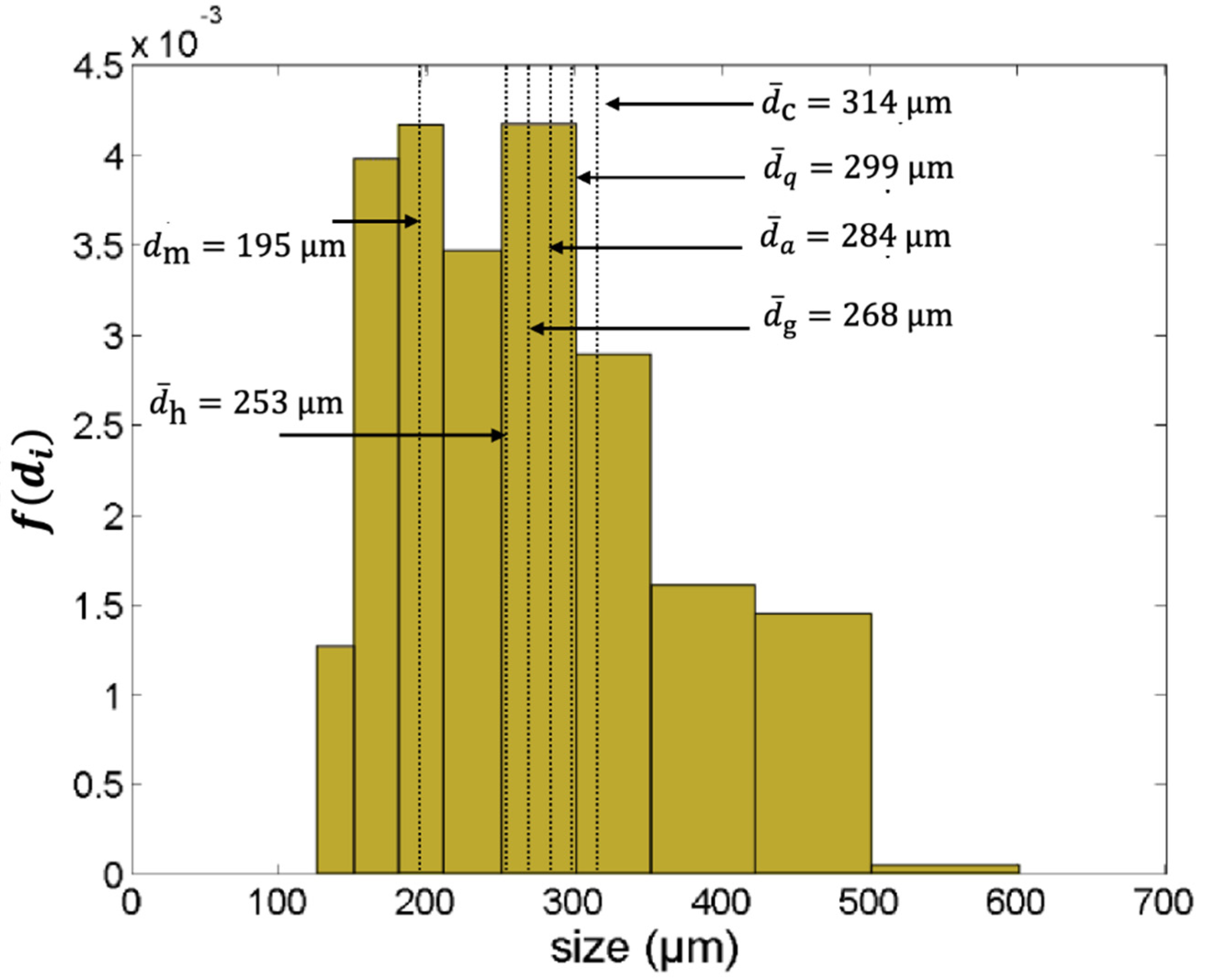
2.1. The Average Particle Size

The determination of the particle size is often the first step in characterizing the particle. For perfect spherical particles, a valid definition of their size would be the diameter of the sphere. In industrial applications, however, perfect spherical particles are seldom encountered. There is no universal definition for particle size when dealing with non-spherical particles. A whole set of definitions is available, each appropriate in specific applications. The most commonly used definitions are listed in Table 1. Additional definitions, such as free-falling diameter, perimeter diameter, Feret’s and Martin’s diameter are seldom used. In view of the growing importance of studying ultrafine airborne particles or drug-delivering aerosols, among others, the aerodynamic and mobility particle diameters are frequently used. The former one is defined as the diameter of a sphere of density 1000 kg/m3 (e.g., the density of water) which settles in still air at the same velocity as the particle in question [13,14,15]. The latter classifies charged particles according to their mobility in an electric field, followed by a particle counter to count particles of a specific mobility [16].

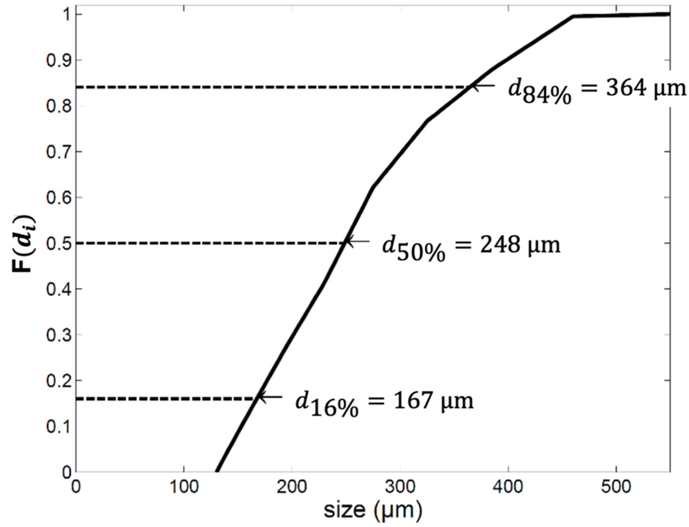
2.2. The Particle Size Distribution

As stated before, the particles of a powder seldom have a uniform size, but are instead characterized by a whole range of particle sizes, representing a size distribution. The knowledge of this size distribution is often of great importance for evaluating powders, for instance, in milled powders where the particle size should not exceed a certain threshold size as determined by quality constraints.
To deal with this problem, the distribution density, f(d), and the cumulative fraction, F(d), are defined. They can be based on the number of particles, although linear (length), square (surface area) or three-dimensional (volume or mass) based distributions are also used. These density functions are indicated by fN(d) and FN(d) for the distribution by numbers; fL(d) and FL(d) for the distribution by length; fs(d) and FS(d) for the distribution by surface area; and fM(d) and FM(d) for a mass distribution. In these definitions, d is the relevant particle size (see Table 1). The distribution by length is seldom used in practice, but is given for reasons of completeness.
For the four possible distribution variants, the distribution density is used to predict the chance that a specific particle size will fall within a certain size interval d { a , b } :
P [ a d b ] = a b f ( d ) d d ,
Or more general: f ( d ) d d is the probability of d falling within the infinitesimal interval [d, d + dd].
The cumulative fraction is defined as follows:
F ( d ) = d f ( d ) d d ,
Since the cumulative fraction integrates the distribution density, the latter can be calculated by taking the derivative of the former.
f ( d ) = dF ( d ) d d ,
In most cases, the size distribution is obtained by experiments that yield a discrete approximation of the distribution. In this approximation, the continuous distribution density, f(d), is divided into I parts i = {1, … , i}, each with a range of sizes of ∆di, an average size di and a value of the distribution f(di). In Equations (4)–(7), the definitions of the discrete distribution densities and the cumulative fraction are given with j as the index of the j-th part of the discrete distribution that corresponds with the value of di:
f N ( d i ) = n i N Δ d i ,   and   F N ( d ) = 0 d f N ( d ) d d i j f N ( d i ) Δ d i
f L ( d i ) = l i L Δ d i ,   and   F L ( d ) = 0 d f L ( d ) d d i j f L ( d i ) Δ d i
f S ( d i ) = s i S Δ d i ,   and   F S ( d ) = 0 d f S ( d ) d d i j f S ( d i ) Δ d i
f M ( d i ) = m i M Δ d i ,   and   F M ( d ) = 0 d f M ( d ) d d i j f M ( d i ) Δ d i
with ni, li, si, mi being the number, length, surface and mass in a size range i and N, L, S and M the total number, length surface and mass.
The different types of distributions are related to each other, by introducing appropriate geometrics shape factors k1, k2 and k3:
f L ( d ) = k 1 d   f N ( d )
f S ( d ) = k 2 d   2 f N ( d )
f M ( d ) = k 3 d   3 f N ( d )
The cumulative distributions are also related to each other and can be based on a continuous frequency distribution or on a discrete approximation:
F L ( d ) = 0 d k 1 d f N ( d ) d d = 0 d k 1 d dF N i j k 1 d i f N ( d i ) Δ d i
F S ( d ) = 0 d k 2 d   2 f N ( d ) d d = 0 d k 2 d 2 dF N i j k 2 d i   2 f N ( d i ) Δ d i
F M ( d ) = 0 d k 3 d   3 f N ( d ) d d = 0 d k 3 d   3 dF N i j k 3 d i   3 f N ( d i ) Δ d i
If the discrete distribution is known, the shape factors can be determined as illustrated below:
f S Δ d i = n i s i i I n i s i = N Δ d i f N ( d i ) s i i I N Δ d i f N ( d i ) s i = f N ( d i ) s i i I f N ( d i ) s i
Let s i = π d i 2 and combined with Equation (3) the shape factor k2 is the following:
k 2 = 1 d i   2 f N ( d i ) Δ d i
The other shape factors are derived in a similar way:
k 1 = 1 d i f N ( d i ) Δ d i
k 3 = 1 d i   3 f N ( d i ) Δ d i
The significance of using the correct base (length, area or volume) will be clarified in the following example for a sieve analysis of a powder with data shown in Table 2.
The volume occupied by the particles is obtained as the ratio of the sieve mass and the absolute density of the particle. The number of particles, n, is obtained by dividing the volume by the volume of one particle, π 6 d 3 with d as the sieve size opening. Additionally, the total particle surface area for a given size is obtained by n π d 2 . The results are shown in Figure 1.
Figure 2 shows that the number and surface area distributions are significantly affected by the smaller particles being present. This is expected, since a small mass of fines contains a large number of particles with a high surface area.
The distribution results can be fitted to a function. A popular fitting equation is the two-parameter log-normal function [18]. Its positive skew describes the commonly encountered phenomenon that more fine particles are measured than larger ones as illustrated in Figure 2.
The log-normal distribution and its cumulative counterpart are given in Equations (18) and (19):
f ( d , μ , σ ) = 1 d σ 2 π exp ( ln ( d μ ) 2 2 σ )
F ( d , μ , σ ) = 1 2 + 1 2 erf ( ln d μ 2 σ 2 )
with µ and σ as the mean and standard deviations of the natural logarithm of the particle size and erf as the error function.
The log-normal distribution function is illustrated in Figure 3 and Figure 4 for different values of µ and σ.
The distribution function is often written in the form of Equation (20), developed by Svarovsky [18]. In this form, the mode dm (the size with maximum distribution density) is used as a parameter instead of the mean.
F ( d , d m , σ ) = a exp ( b ln 2 ( d d m ) )
with
a = 1 d m b π exp ( 1 4 b ) ,   b = 1 2 ln 2 ( σ )
Instead of trying to fit the distribution data, it is also possible to summarize them in some key numbers such as the mean, modus, median and spread.
Because of this wide variety of definitions, the calculation of the mean can be somewhat confusing. In general, the calculation of the mean is defined as in Equation (21).
g ( d ¯ ) = 0 g ( d ) f ( d ) d d i I g ( d i ) f ( d i ) Δ d i
with di as the average size in an increment range of size ∆di.
Depending on the application, different functions of g(d) are used, as listed in Table 3.
Other indicators of the average particle size in a powder are the modus and mean. The modus (dm) is, as already stated, the most commonly found size in the distribution. As opposed to the mean and the modus, the median (d50%) is most easily identified using the cumulative fraction, F(d), where it corresponds to the 50 %-value.
An indication of the size distribution is given by the spread, σ, and the relative spread, σ/d50%, with the following definitions:
σ = d 84 % d 16 % 2
σ d 50 % = d 84 % d 16 % 2 d 50 %
In Equations (22) and (23), d84% and d16% correspond with the particle size with a cumulative fraction F(d) equal to 84 % and 16 %, respectively. Some particle size analyzers (e.g., laser diffraction) use a slightly different definition with the spread evaluated between d90% and d10%.
The mean, median, modus and spread are illustrated by a sieving test. A sand mixture was sieved and analyzed with the results presented in Table 4.
Based on this data, using Equation (7), the distribution and cumulative fraction was calculated. The results from these calculations are presented in Figure 5 and Figure 6. Additionally, the different kinds of means, the median, the modus and the spread were calculated. Note that the size range ∆di is not uniform.

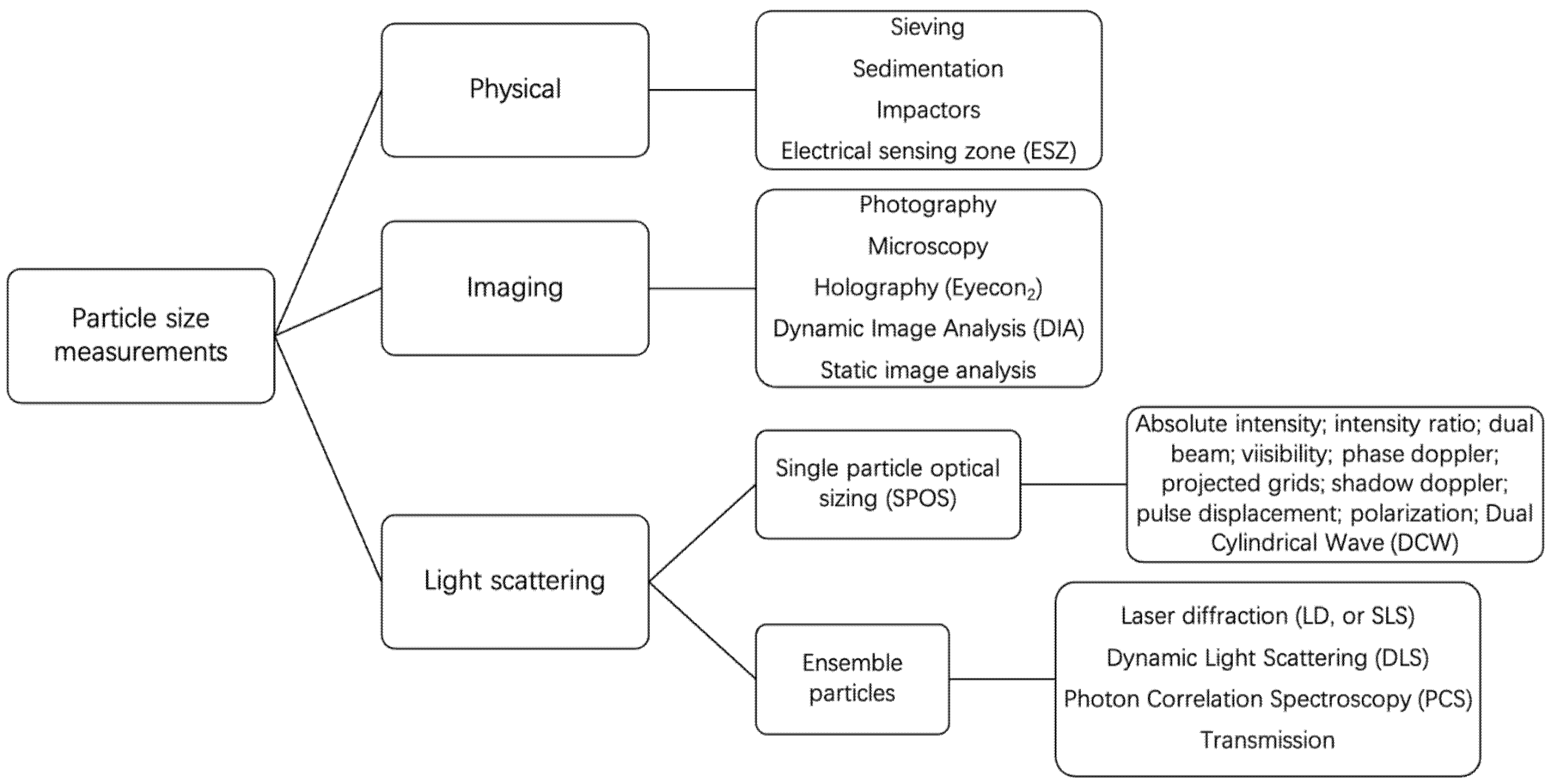
2.3. Particle Size and Size Distribution Measurements

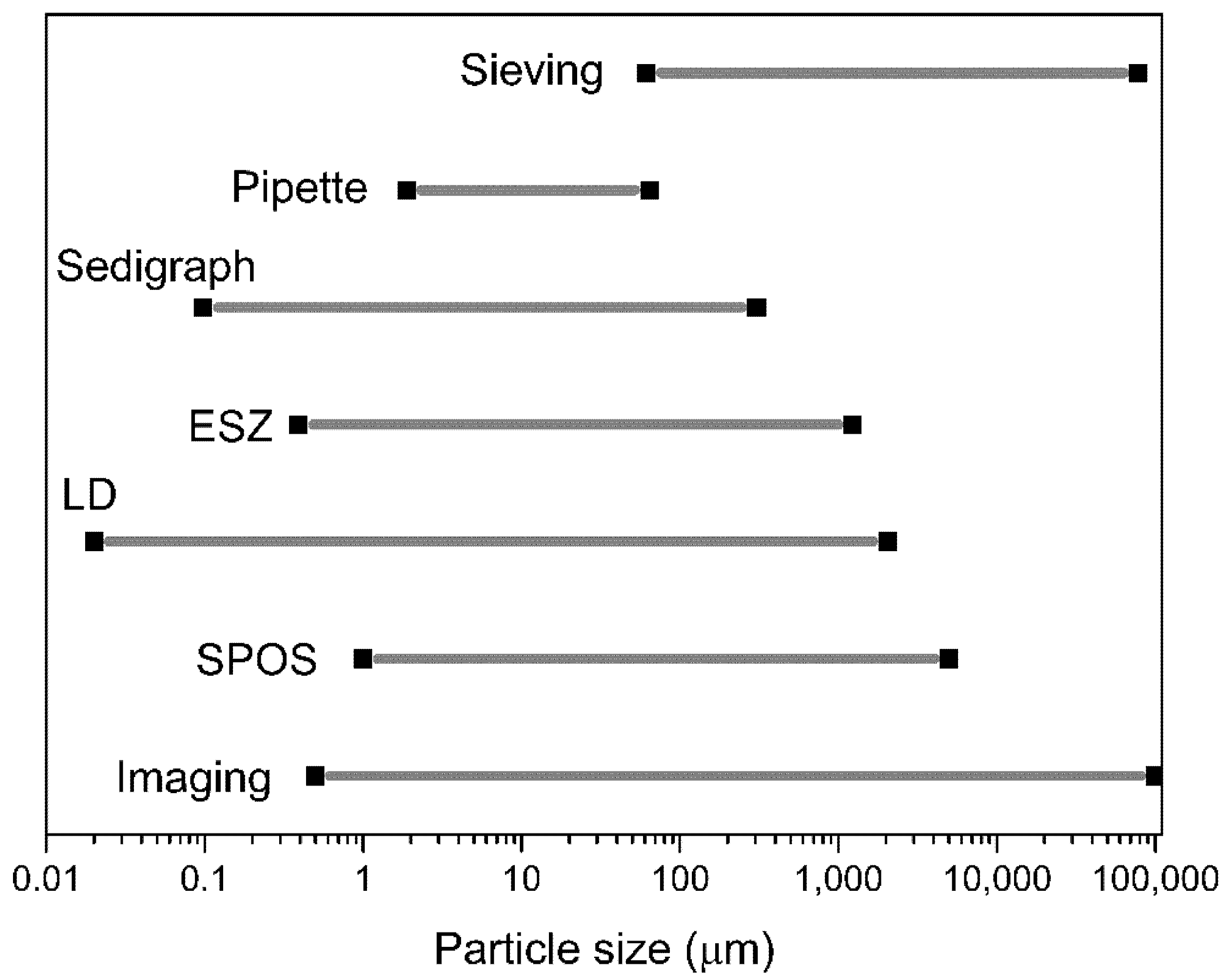
2.3.1. Common Instrumental Techniques

Different methods of measurement can be used, as depicted in Figure 7 [19,20,21,22,23].
Each method covers a characteristic size range within which measurement is possible. These ranges partly overlap, as is shown in Figure 8. However, the results for measuring the same sample vary considerably. In some of the techniques, except imaging-based ones, the PSD is affected by the random orientation of particles during measurements. In principle, image analysis is preferred to provide physically relevant particle sizes of well-dispersed, irregularly shaped particles.
Each method provides different sizes and PSD types, as illustrated in Table 5.

2.3.2. Parameters Affecting the Instrumental Particle Size Measurement

Although the particle size analysis is expected to accurately measure the particle size distribution in any size range, repeat measurements often differ. It is imperative to respect rules regarding the sample preparation, the measurement procedure and the analyzers themselves. Standard methods should hence be used. Instrument specifications should be accounted for and the results’ presentation should be standardized. Various ISO standards were already referred to in the introduction of the paper. An extensive research of Zhang et al. [25] investigated the major parameters to be considered. The main conclusions of the study are highlighted below and consider parameters of Table 6.
Although demi-water is mostly used for insoluble materials, its pH needs to be pH-adapted to be in line with the zeta-potential of the particles. Denser insoluble particles will need to use organic liquids of appropriate density as solvents. Iso-propanol and aromatics are frequently used. Alcohols promote the de-agglomeration of particles. Acetone or aromatics tend to provoke particle adhesion on the cell wall, thus hampering measurement reproducibility. Normally, a 25 vol% of iso-propanol is selected.
Different particles and different solvents call for different dispersants. Polyphosphates are commonly applied for insoluble materials, with hexa-metaphosphate as the most effective, although it loses its activity within 24 h. The type of dispersant and its concentration should reduce the zeta-potential, preferably to below −60 mV, and should avoid obscuration and sedimentation. Normally, a concentration of 100 ppm would lower the zeta-potential to below ~60 mV. An over-dosage could however lead to particle agglomeration rather than dispersion. Low-molecular-weight organic dispersants, such as Daxad 11G [26], are valid alternatives and can be applied at concentrations of about 1 wt%.
Beside using dispersants, particle samples should be mechanically de-agglomerated during the measurement by either ultrasonic or mechanical mixing. The mixing energy input should be limited to avoid particle attrition or disintegration. Both mechanical and ultrasonic mixing are provided in commercial equipment. The sonication output power is normally set at about 200 to 300 W, and the sonication duration has a limited effect only if exceeding 0.5 to 1 min.
The particle refractive index considerably affects the sizing results, although results for a refractive index in excess of 1.8 to 2 hardly affect the results. Particle refractive index values are listed in several handbooks such as [26].
The amount of sample is critical, with excess sample leading to agglomeration. A concentration of 2 g/L is recommended.
These findings and recommendations were confirmed by several researchers with respect to the medium of suspension and dispersant [27,28]. Vdovic et al. [29] investigated the effects of sample pre-treatment with dispersant. Storti and Balsamo [30] investigated the effect of dispersing methods for sands, whereas Schulte and Lehmkuhl [31] assessed the differences in results by the Mie and Fraunhofer theory. Yang et al. [32] found minor differences of PSD results between the laser diffraction sieve–pipette method.
Although each technique has its own basis (mass, number, volume) where it yields the most reliable data, results will be fairly comparable if presented on the same basis and scale in a logarithmic or normalized distribution, even for very wide PSD [33,34,35].

2.3.3. Comparing the Common Particle Size Analyzers

Some particle analyzers were tested for 2 powders, i.e., Al2O3 (3 130 kg/m3) and SiC (3 960 kg/m3), with additional properties given in Table 7 [25]. Ten measurements were carried out. The results and coefficients of variation are given in Table 8.
The coefficients of variation of d50 are generally less than 10%, except for photo-sedimentation with a ~20% relative accuracy.

3. Particle Shape

It was already clear from the multiple particle size definitions in the previous section that perfectly spherical particles are a curiosity. However, correctly quantifying the shape of particles in practice proves to be quite difficult. A commonly used concept is the sphericity, ψ (−), of a particle.
ψ = surface   area   of   a   sphere   with   the   same   volume   as   the   particle surface   area   of   the   particle
It can be shown that
ψ = d sv d v
For particles with regular shapes, the sphericity can theoretically be calculated from the geometry using Equation (25). Some correlations are given in Table 9.
For non-regularly shaped particles, both the volume diameter (dv) and the surface to volume diameter (dsv) have to be determined experimentally.
The volume diameter can be calculated with following formula:
d v = [ 6 M ρ p π n ] 1 / 3
with M being the total mass (kg) and n the number of particles in the examined powder and ρ p , the particle density (kg/m3), which will be discussed in detail in the following section.
The surface-to-volume ratio can be determined with a pressure-drop experiment. In this experiment, the powder is put in a circular tube through which a gas is blown at low flow rates and the occurring pressure gradients are measured. For a low Reynolds, the Carman-Kozeny equation relates the measured pressure gradient to the bed voidage:
If
Re = ρ g ν d sv μ < 2
Then
Δ p L = 150 ( 1 ε ) 2 ε 3 μ ν d sv 2
with ∆p being the pressure drop (Pa), L the bed depth (m), ε the bed voidage (-), µ the gas viscosity (Pa s) and ν the superficial velocity (m/s).
The sphericity of some common materials is listed in Table 10.

4. Particle Density and Bed Voidage

The knowledge of particle and bed density is in many applications a requisite with the obvious examples of fixed beds, fluidized beds and compaction processes.
The particle density, ρ p (kg/m3), bed bulk density, ρ B (kg/m3), density of the fluid occupying the intra- and interparticle empty space, ρ g , and bed voidage, ε (−), are correlated by:
ρ B = ε ρ g + ( 1 ε ) ρ p   with   ρ g 0 ,   ε = 1 ρ B / ρ p
The approximation that ρ g is nearly zero is justified for a gas as fluid.
The particle density in Equation (29) should not be confused with the absolute or skeletal density, ρ abs (kg/m3), of the material out of which the particle is composed. Due to a possible internal porous structure of the particle, the particle density will often be lower than the absolute density. Sometimes the particle density is denoted with other names such as hydrodynamic, apparent, envelope, effective or piece density [38,39].

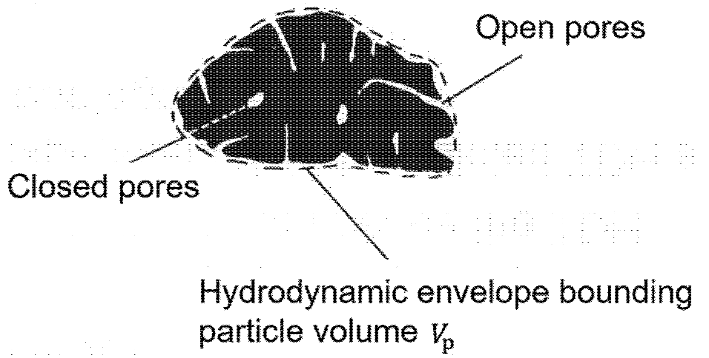
4.1. Particle Density

An accurate measuring of the particle density can be quite difficult, especially if the particle is highly porous, as illustrated in Figure 9. This is exemplified by the disrupting influence of humidity on measurements. In a humid atmosphere, water will adsorb in the porous with the amount of condensed liquid being a function of relative humidity, pore diameter and surface tension.
In the case of porous particles, the particle density is a ratio of the mass to the hydrodynamic envelope bounding particle volume, ρ p = M / V p .
In general, 7 methods or measuring devices can be distinguished to determine the particle density: (i) caking end-point measurements, (ii) mercury porosimeters, (iii) comparative measurements, (iv) gas flow measurements, (v) powder displacement measurements, (vi) minimum fluidization velocity measurements and (vii) photographic measurements.
(1)
Caking end-point measurements are sometimes performed in the petrochemical industry for rapid and cheap estimations of pore volume. In these measurements, the investigated powder is put in a vibrating flask and a liquid with low viscosity or volatility (for example, water) is added incrementally. As long as the liquid is absorbed into the microscopic pores, the powder remains free-flowing. If the pores are completely filled, any surplus of liquid will coat the surface of the particles and cause the formation of liquid bridges, i.e., caking. This surplus depends on pore size and the surface tension. A complete filling-up of the pores is often impossible due to surface tension constraints. As a result, the caking end-point measurement method tends to overestimate the particle density. If the pore volume is determined, the particle density can be calculated with:
ρ p = 1 x + 1 / ρ abs
with x as the specific pore volume (m3/kg).
The absolute density ( ρ abs ) can be measured with a balance (absolute mass) and pycnometer (absolute volume).
(2)
In a porosimeter, mercury under high pressure is forced into to the pores of the particles. Eventually, the pore size can be determined. As in the caking end-point method, the particle density is determined from Equation (30). A major setback of this measuring method is its high cost.
(3)
The particle density can also be determined in the comparative method by examining the tapped bulk density, ρ BT , of both the sample and a control powder. Then, applying Equation (31) yields the particle density of the investigated sample powder.
ρ pX = k ρ BTX ρ BTC ρ pc
with ρ BTX and ρ BTC as the tapped bulk density of the sample and the control powder and ρ pC and ρ pX as the particle density of the sample and control powder. Since the control powder might have a different particle shape than that of the unknown powder, a shape factor k is introduced, with illustrative values as given below:
  • k = 1    for identically shaped sample particles and control particles
  • k ≈ 0.82  for rounded or spherical sample particles and angular control particles
  • k ≈ 1/0.82  for angular sample particles and spherical or rounded control particles
(4)
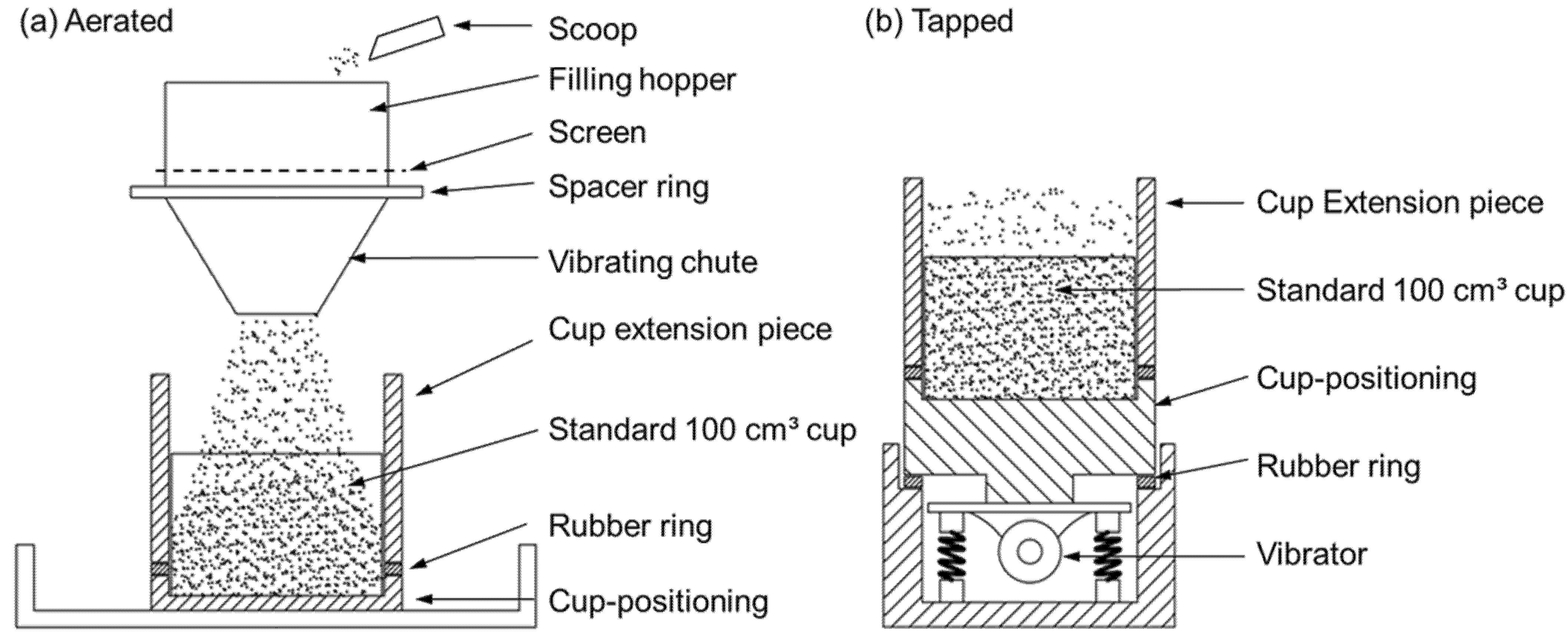
In the adapted gas flow technique of Ergun, the particle density is determined by comparing the pressure drop over a bed with minimum voidage to a bed with a maximum voidage. Maximum voidage can be achieved by fluidizing the sample and letting it gently settle. The resulting bed can next be tapped for a sufficient length of time to reach the state of minimal voidage. In both situations, the bed height LA (aerated) and LT (tapped) is measured. Additionally, the pressure drop, ∆p, is recorded for at least four different gas velocities. Next, the pressure drop is plotted against the superficial velocity (v) and the slope within the laminar flow regime (Re < 2) is measured. With these values, the particle density can be calculated using a rearranged form of Equation (28), i.e., the Ergun equation in the laminar flow regime, with L, the bed length (m), ε the bed voidage (-) and µ the gas viscosity (Pa s).
(5)
Rearranged, the slopes of the graphs SA and SB for the two beds are
S A = [ Δ p v ] T = 150 μ d sv 2 L A ( 1 ε A ) 2 ε A 3
S T = [ Δ p v ] T = 150 μ d sv 2 L T ( 1 ε T ) 2 ε T 3
L A L T = ρ BT ρ BA
1 ε A = ρ BA ρ P
1 ε T = ρ BT ρ P
Dividing Equation (32) by Equation (33) and substituting LA, LT, εA and εT, yields:
S A S T = ρ BA ρ BT ( ρ P ρ BT ρ P ρ BA ) 3
ρ P can be calculated with:
Y = S A S T ρ BT ρ BA
ρ P = ρ BT Y 1 / 3 ρ BA 1 Y 1 / 3
Since the method requires an accurate measurement of the pressure drop, caution should be made when dealing with cohesive powders as channeling is likely to occur.
(6)
In the powder displacement method, the particle density is measured by comparing the tapped bulk density of a control powder with a mixture of the control and the sample powder. This technique is specific because the fine powder is used as pycnometric fluid to fill the open pores in the investigated particles. As such, the pycnometric powder must be free-flowing, non-porous and sufficiently smaller than the sample particles. If the latter condition is not fulfilled, the comparison between the control powder and the mixture of control and sample powder will give erroneous results. This test can be performed in the apparatus illustrated in Figure 10b. If the control tapped bulk density is ρ BTC , up to 20 wt% of the larger unknown porous particles is mixed with the control powder and tapped in the cup of Figure 10b.
Additional control powder is added and tapped to completely fill the cup. The resulting mixture is weighed and as such, the added mass of control powder, Mc, is determined. With this, the particle density of the unknown particles, ρ pX , is determined with Equation (40):
ρ px = M x ( V M c / ρ BTC )
with Mx being the mass of sample in the mixture and V the volume of the cup.
(7)
Additionally, the minimum fluidization velocity is related to the particle density in the Ergun equation:
ρ p = [ 1.75 ε MF 3 [ d sv ν MF ρ g μ ] 2 + 150 ( 1 ε MF ) ε MF 3 [ d sv ν MF ρ g μ ] ] μ 2 d sv 3 ρ g g + ρ g
with the subscript MF denoting the conditions at minimum fluidization velocity.
The voidage εMF itself is dependent on the particle density as follows:
ε MF = 1 ρ BMF ρ p
The solution of Equations (41) and (42) is found via an iterative procedure.
This technique proposed is only valid for spherical particles. Also, accurate values of size dsv are required. The latter is not troublesome for spherical particles since the sieve size da in that case equals the surface-to-volume ratio, dsv.
ρ p = [ 1.75 ψ ε MF 3 [ x sv ν MF ρ g μ ] 2 + 150 ( 1 ε MF ) ψ 2 ε MF 3 [ x sv ν MF ρ g μ ] ] μ 2 x sv 3 ρ g g + ρ g
(8)
Finally, for reasons of completeness, the photographic technique is mentioned here. For a full description, the reader is advised to review the description given by Li and Iskander [42] and Grace and Ebneyamini [43]. A summary of the techniques is given in Table 11.

4.2. Bulk Density

The bulk density relates the mass of a powder to its bulk volume. With this definition, the bulk density is dependent on the size, size distribution, shape and the state of compaction of the particles. The latter can be thought of as non-material dependent, but rather as an operating or measuring condition. As such, caution must be taken that the same standardized measurement method is applied when comparing different bulk densities.
The state of compaction of the particles gives way to four categories of bulk densities: aerated or most loosely packed bulk density ρ BLP , poured bulk density ρ BP , tapped bulk density ρ BT and compacted bulk density ρ BC . For identical powders (equal composition, size, size distribution and shape), the values of the different categories of bulk density are obviously in the following order:
ρ BLP < ρ BP < ρ BT < ρ BC
Most often, only the aerated and the tapped bulked density are used.
The ratio of the tapped to the aerated bulk density is called the Hausner ratio, ρ BT / ρ LP , and gives a measure of the powder flowability vs. cohesivity. For instance, powders with strong interparticle forces will exhibit a relatively open structure if little or no work is done on the powder. However, tapping will compact them to a dense structure which corresponds to a high Hausner ratio. On the other hand, free-flowing powders with little or no interparticle forces will exhibit low values of the Hausner ratio. According to the Hausner ratio (RH), powders can be classified in different categories:
  • RH < 1.25:     Group A, B, or D
  • RH > 1.4:    Group C
  • 1.25 < RH < 1.4:  Transition group AC
Both the aerated and the tapped bulk densities can be measured with the apparatus depicted in Figure 10. In Figure 10a, the aerated bulk density is determined by pouring the powder through a vibrating sieve which subsequently falls through the vibrating and stationary chutes into a cylindrical cup. The filling of the cup should take about 20–30 s. Any excess powder on top is removed and the cup is weighed. With the known mass of the powder, the aerated density is calculated. Next, an extension piece is attached to the full cup, as illustrated in Figure 10b. Subsequently, the cup is tapped 480 times whilst extra powder is added to fill the cup completely. After tapping, the extension is removed and excess powder on top of the cup is scraped off. Finally, the mass of the tapped powder is weighed and the tapped bulk density is calculated.

4.3. Bed Voidage

The bed voidage ε can be evaluated with Equation (29) if the particle and bulk densities ρ P and ρ B are known, but some general remarks about influencing factors can be made.
Factors that influence voidage are:
  • The compaction state: Obviously, a tapped bed will have a smaller voidage than an aerated bed. Two extreme conditions, assuming random packing, are used as a reference: ‘loose’ packing with the maximum voidage and ‘dense’ packing with minimum voidage.
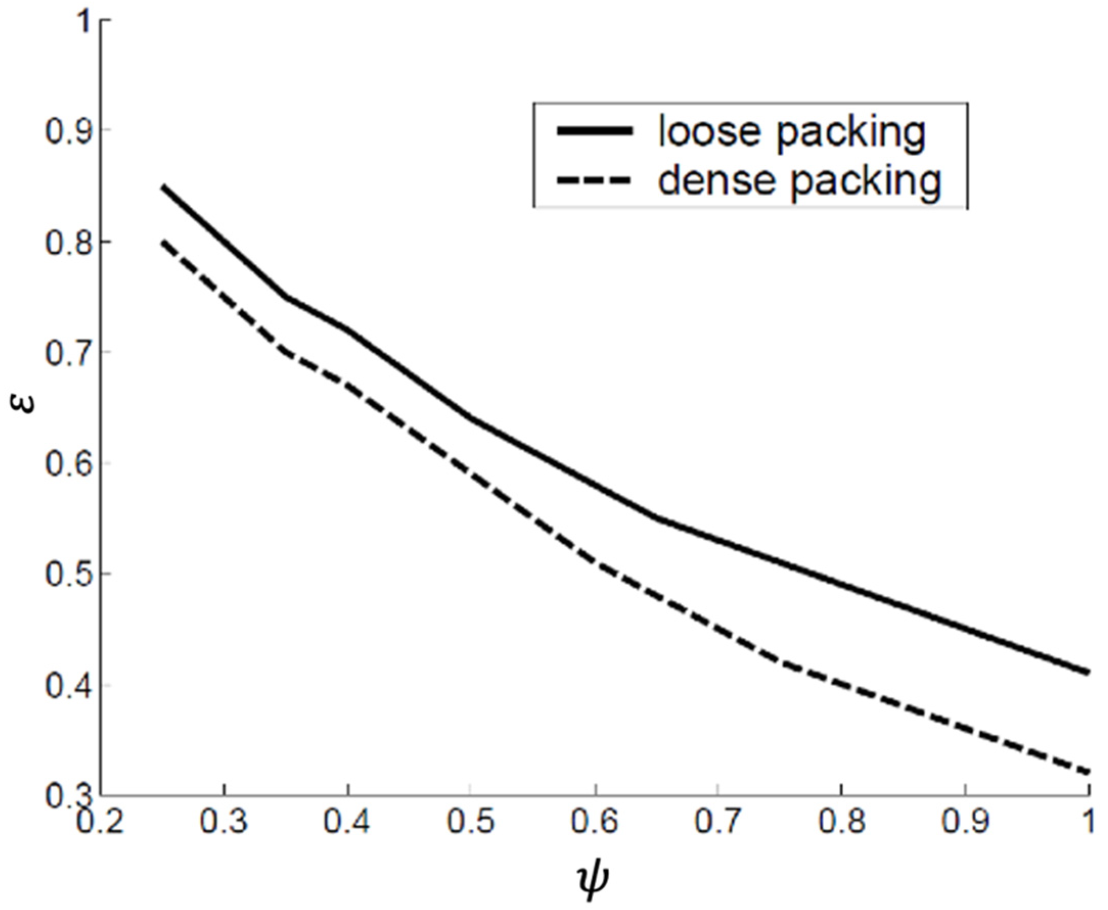
  • The particle shape: The voidage increases with decreasing sphericity. This is illustrated in Figure 11.
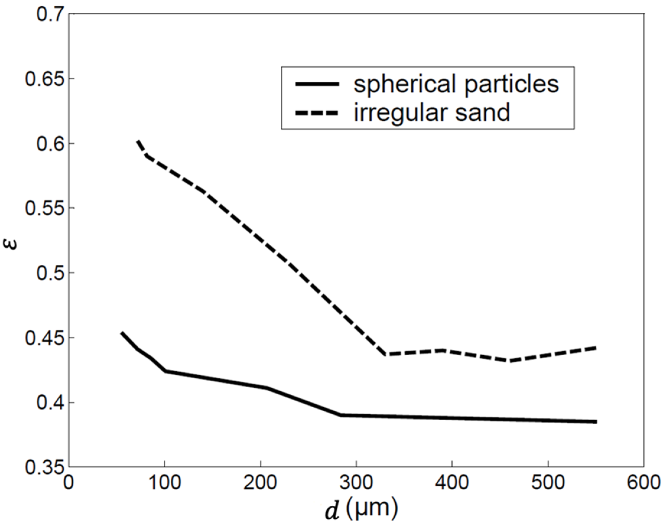
  • The particle size: For loosely packed beds, the voidage decreases with increasing particle size. The densely packed bed voidage, on the other hand, is quite insensitive to size. This is illustrated in Figure 12.
  • The particle size distribution: The voidage decreases with increasing spread.
  • The particle and wall roughness: The voidage increases with increasing surface roughness.

5. Conclusions

The design of fluid–solid processes relies on the accurate measurement of particle properties (size, size distribution, absolute and bulk density and shape).
The research discussed methods to define and measure these properties.
Particle size and its size spread is commonly measured by instrumental techniques. Recommendations towards sample size, selected solvents and dispersants and suspension mixing were defined. Size distribution functions are strongly affected by the quantity of fine particles present in the sample.
The particle shape is expressed as its sphericity. Although it is difficult to measure the sphericity, microscopic imaging or pressure drop measurements across a fixed particle bed can be used.
The absolute, apparent and bulk density of particles and powders can be determined by seven different methods. The bulk density determines the voidage of a particle assembly.

Author Contributions

The conceptualization of the research was performed by Y.D., R.D. and J.B. The methodology was set by L.A., H.Z. and S.L. All authors participated in the validation and original draft preparation. Y.D. and J.B. were co-responsible for the writing—review and editing. J.B. was responsible for the funding acquisition and project administration. All authors have read and agreed to the published version of the manuscript.

Funding

This research was supported by The Beijing Advanced Innovation Centre of Smart Matter Science and Engineering of the Beijing University of Chemical Technology, Beijing, China.

Institutional Review Board Statement

Not applicable.

Informed Consent Statement

Not applicable.

Data Availability Statement

Excluded, since data are examples only.

Conflicts of Interest

The authors declare no conflict of interest.

References

  1. Deng, Y.; Sabatier, F.; Dewil, R.; Flamant, G.; Le Gal, A.; Gueguen, R.; Baeyens, J.; Li, S.; Ansart, R. Dense upflow fluidized bed (DUFB) solar receivers of high aspect ratio: Different fluidization modes through inserting bubble rupture promoters. Chem. Eng. J. 2021, 418, 129376. [Google Scholar] [CrossRef]
  2. Deng, Y.; Dewil, R.; Appels, L.; Li, S.; Baeyens, J.; Degrève, J.; Wang, G. Thermo-chemical water splitting: Selection of priority reversible redox reactions by multi-attribute decision making. Renew. Energy 2021, 170, 800–810. [Google Scholar] [CrossRef]
  3. Li, S.; Baeyens, J.; Dewil, R.; Appels, L.; Zhang, H.; Deng, Y. Advances in rigid porous high temperature filters. Renew. Sustain. Energy Rev. 2021, 139, 110713. [Google Scholar] [CrossRef]
  4. Liu, J.; Baeyens, J.; Deng, Y.; Tan, T.; Zhang, H. The chemical CO2 capture by carbonation-decarbonation cycles. J. Environ. Manag. 2020, 260, 110054. [Google Scholar] [CrossRef] [PubMed]
  5. Deng, Y.; Ansart, R.; Baeyens, J.; Zhang, H. Flue Gas Desulphurization in Circulating Fluidized Beds. Energies 2019, 12, 3908. [Google Scholar] [CrossRef] [Green Version]
  6. Zhang, H.; Degrève, J.; Baeyens, J.; Dewil, R. The Voidage in a CFB Riser as Function of Solids Flux and Gas Velocity. Procedia Eng. 2015, 102, 1112–1122. [Google Scholar] [CrossRef] [Green Version]
  7. Zhang, H.L.; Baeyens, J.; Degrève, J.; Brems, A.; Dewil, R. The convection heat transfer coefficient in a Circulating Fluidized Bed (CFB). Adv. Powder Technol. 2014, 25, 710–715. [Google Scholar] [CrossRef]
  8. ISO 13317-4:2014(en). Determination of Particle Size Distribution by Gravitational Liquid Sedimentation Methods. Available online: https://www.iso.org/obp/ui/#!iso:std:46263:en (accessed on 30 July 2021).
  9. ISO 13320:2020. Particle Size Analysis—Laser Diffraction Methods. 2020. Available online: https://www.iso.org/standard/69111.html (accessed on 30 July 2021).
  10. ISO 19.120. Particle Size Analysis.Sieving-Including Test Sieves and Porosimetry. 2020. Available online: https://www.iso.org/ics/19.120/x/ (accessed on 30 July 2021).
  11. ISO 9276-2:2014. Representation of Results of Particle Size Analysis—Part 2: Calculation of Average Particle Sizes/Diameters and Moments from Particle Size Distributions, Reviewed and Confirmed in 2019. Available online: https://www.iso.org/standard/57641.html (accessed on 30 July 2021).
  12. ISO 9276-6:2008 Representation of Results of Particle Size Analysis—Part 6: Descriptive and Quantitative Representation of Particle Shape and Morphology, Reviewed and Confirmed in 2017. Available online: https://www.iso.org/standard/39389.html (accessed on 30 July 2021).
  13. Sundahl, M.; Berg, E.; Svensson, M. Aerodynamic particle size distribution and dynamic properties in aerosols from electronic cigarettes. J. Aerosol Sci. 2017, 103, 141–150. [Google Scholar] [CrossRef]
  14. Miyamoto, K.; Taga, H.; Akita, T.; Yamashita, C. Simple Method to Measure the Aerodynamic Size Distribution of Porous Particles Generated on Lyophilizate for Dry Powder Inhalation. Pharmaceutics 2020, 12, 976. [Google Scholar] [CrossRef] [PubMed]
  15. Sjoholm, P.; Ingham, D.B.; Lehtimaki, M.; Perttu-Roiha, L.; Goodfellow, H.; Torvela, H. Gas-Cleaning Technology. In Industrial Ventilation Design Guidebook; Elsevier: Amsterdam, The Netherlands, 2001; pp. 1197–1316. [Google Scholar]
  16. Centre for Atmospheric Science Differential Mobility Particle Sizer (DMPS). Available online: http://www.cas.manchester.ac.uk/restools/instruments/aerosol/differential/ (accessed on 30 July 2021).
  17. Svarovsky, L. Solid-Liquid Separation, 3rd ed.; Butterworths: London, UK, 1990. [Google Scholar]
  18. Svarovsky, L. A contribution to the use of the log-probability paper for particle size measurement. Powder Technol. 1973, 7, 351–352. [Google Scholar] [CrossRef]
  19. Dukhin, A.S.; Goetz, P.J.; Fang, X.; Somasundaran, P. Monitoring nanoparticles in the presence of larger particles in liquids using acoustics and electron microscopy. J. Colloid Interface Sci. 2010, 342, 18–25. [Google Scholar] [CrossRef]
  20. Naito, M.; Hayakawa, O.; Nakahira, K.; Mori, H.; Tsubaki, J. Effect of particle shape on the particle size distribution measured with commercial equipment. Powder Technol. 1998, 100, 52–60. [Google Scholar] [CrossRef]
  21. Tinke, A.P.; Govoreanu, R.; Vanhoutte, K.; Brewster, M. Particulate system characterization: Evaluation of particle size distribution data. Am. Pharm. Rev. 2007, 10, 68. [Google Scholar]
  22. Strokotov, D.I.; Moskalensky, A.E.; Nekrasov, V.M.; Maltsev, V.P. Polarized light-scattering profile-advanced characterization of nonspherical particles with scanning flow cytometry. Cytom. Part A 2011, 79A, 570–579. [Google Scholar] [CrossRef] [PubMed]
  23. Saveyn, H.; Thu, T.L.; Govoreanu, R.; Meeren, P.; Vanrolleghem, P.A. In-line Comparison of Particle Sizing by Static Light Scattering, Time-of-Transition, and Dynamic Image Analysis. Part. Part. Syst. Charact. 2006, 23, 145–153. [Google Scholar] [CrossRef]
  24. Abbireddy, C.O.R.; Clayton, C.R.I. A review of modern particle sizing methods. Proc. Inst. Civ. Eng. Geotech. Eng. 2009, 162, 193–201. [Google Scholar] [CrossRef]
  25. Zhang, H.; Baeyens, J.; Kang, Q. Measuring Suspended Particle Size with High Accuracy. Int. J. Petrochem. Sci. Eng. 2017, 2. [Google Scholar] [CrossRef] [Green Version]
  26. Lide, D.R. (Ed.) CRC Handbook of Chemistry and Physics, 85th ed.; Chemical Rubber Company Press: Baco Raton, FL, USA, 2004. [Google Scholar]
  27. Chappell, A. Dispersing sandy soil for the measurement of particle size distributions using optical laser diffraction. CATENA 1998, 31, 271–281. [Google Scholar] [CrossRef]
  28. Beuselinck, L.; Govers, G.; Poesen, J.; Degraer, G.; Froyen, L. Grain-size analysis by laser diffractometry: Comparison with the sieve-pipette method. CATENA 1998, 32, 193–208. [Google Scholar] [CrossRef]
  29. Vdović, N.; Obhođaš, J.; Pikelj, K. Revisiting the particle-size distribution of soils: Comparison of different methods and sample pre-treatments. Eur. J. Soil Sci. 2010, 61, 854–864. [Google Scholar] [CrossRef]
  30. Storti, F.; Balsamo, F. Particle size distributions by laser diffraction: Sensitivity of granular matter strength to analytical operating procedures. Solid Earth 2010, 1, 25–48. [Google Scholar] [CrossRef] [Green Version]
  31. Schulte, P.; Lehmkuhl, F. The difference of two laser diffraction patterns as an indicator for post-depositional grain size reduction in loess-paleosol sequences. Palaeogeogr. Palaeoclimatol. Palaeoecol. 2018, 509, 126–136. [Google Scholar] [CrossRef]
  32. Yang, Y.; Wang, L.; Wendroth, O.; Liu, B.; Cheng, C.; Huang, T.; Shi, Y. Is the Laser Diffraction Method Reliable for Soil Particle Size Distribution Analysis? Soil Sci. Soc. Am. J. 2019, 83, 276–287. [Google Scholar] [CrossRef]
  33. Sousan, S.; Regmi, S.; Park, Y.M. Laboratory Evaluation of Low-Cost Optical Particle Counters for Environmental and Occupational Exposures. Sensors 2021, 21, 4146. [Google Scholar] [CrossRef]
  34. Kubínová, R.; Neumann, M.; Kavka, P. Aggregate and Particle Size Distribution of the Soil Sediment Eroded on Steep Artificial Slopes. Appl. Sci. 2021, 11, 4427. [Google Scholar] [CrossRef]
  35. Galacgac, J.A.; Ooi, P.S.K. Use of a Laser Diffractometer to Obtain the Particle Size Distribution of Fine-Grained Soils. Transp. Res. Rec. J. Transp. Res. Board 2018, 2672, 1–11. [Google Scholar] [CrossRef]
  36. Perry Perry’s chemical engineers’ handbook. Choice Rev. Online 1998, 35. [CrossRef] [Green Version]
  37. Mc Cabe, W.L.; Smith, J.C.; Harriott, P. Unit Operation of Chemical Engineering, 5th ed.; McGraw-Hill: New York, NY, USA, 1993. [Google Scholar]
  38. Jurtz, N.; Wehinger, G.D.; Srivastava, U.; Henkel, T.; Kraume, M. Validation of pressure drop prediction and bed generation of fixed-beds with complex particle shapes using discrete element method and computational fluid dynamics. AIChE J. 2020, 66, e16967. [Google Scholar] [CrossRef]
  39. Koekemoer, A.; Luckos, A. Effect of material type and particle size distribution on pressure drop in packed beds of large particles: Extending the Ergun equation. Fuel 2015, 158, 232–238. [Google Scholar] [CrossRef]
  40. Geldart, D. Gas Fluidization Technology; John Willy & Sons: Chichester, UK, 1986. [Google Scholar]
  41. Santomaso, A.C.; Lazzaro, P.; Canu, P. Powder flowability and density ratios: The impact of granule packing. Chem. Eng. Sci. 2003, 58, 2857–2874. [Google Scholar] [CrossRef]
  42. Li, L.; Iskander, M. Comparison of 2D and 3D dynamic image analysis for characterization of natural sands. Eng. Geo. 2021, 290, 106052. [Google Scholar] [CrossRef]
  43. Grace, J.R.; Ebeyamini, A. Connecting particle sphericity and circularity. Particuology 2021, 54, 1–4. [Google Scholar] [CrossRef]
  44. Montillon, G.H. Unit Operations. By G. G. Brown, A. S. Foust, D. L. Katz, R. Schneidewind, R. R. White, W. P. Wood, J. T. Banchero, G. M. Brown, L. E. Brownell, J. J. Martin, G. B. Williams, and J. L. York. J. Phys. Chem. 1951, 55, 614–616. [Google Scholar] [CrossRef]
Figure 1. Number, area and volume fractions.
Standards 01 00004 g001
Figure 2. Number, area and volume size distributions.
Standards 01 00004 g002
Figure 3. Log-normal distribution for different values of µ and σ   = 1.0.
Standards 01 00004 g003
Figure 4. Log-normal distribution for different values of σ, for a constant µ = ln(20 000).
Standards 01 00004 g004
Figure 5. Distribution f(di) of the sieved sand with indications of the different mean values, with the modus, dm; and d a ¯ ,   d q ¯ ,   d c ¯ ,   d h ¯ ,   d g ¯ as arithmetic, quadratic, cubic, harmonic and geometric means.
Standards 01 00004 g005
Figure 6. Cumulative fraction with indications of the median d50% and the fractions d16% and d84%. The spread σ is 197 µm while the relative spread σ/d50% equals 0.79.
Standards 01 00004 g006
Figure 7. Particle size distribution measurements.
Standards 01 00004 g007
Figure 8. Measuring ranges of the various techniques, with acronyms of Figure 7 (adapted from [24]).
Standards 01 00004 g008
Figure 9. A porous particle.
Standards 01 00004 g009
Figure 10. Measurement of aerated and tapped bulk density (adapted from [40,41]).
Standards 01 00004 g010
Figure 11. Voidage versus sphericity for loosely and densely packed beds of uniformly sized particles larger than about 500 µm [44].
Standards 01 00004 g011
Figure 12. Variation of packed bed voidage vs. particle size for spherical particles and sand. The particle size distribution is narrow in both cases.
Standards 01 00004 g012
Table 1. Definitions of the particle diameter (adapted from [17]).
SymbolDiameter DefinitionEquivalent Sphere Diameters
dASieve Largest sphere diameter that can pass through the square aperture of the sieve.
dvVolume Sphere diameter when particle and sphere volumes are equal.
dsSurface Sphere diameter when particle and sphere surfaces are equal.
dSVSurface to Volume Sphere diameter when the surface area to volume ratio of the sphere and the particle are equal.
Table 2. Results of a sieve analysis for particles with absolute density of 2 600 kg/m3.
Sieve Size (mm)Average Size (mm)Sieve Mass (g)Mass Fraction
0.04–0.060.050.10.03
0.06–0.100.080.40.11
0.010–0.180.140.70.19
0.18–0.300.240.90.25
0.30–0.420.360.70.19
0.42–0.590.50.50.14
0.59–0.830.710.20.06
0.83–1.000.920.10.03
Total 3.61
Table 3. Different means and distribution functions.
Meang(d)Formula
Arithmetic d d ¯ a = i d i f ( d i ) Δ d i
Quadratic d2 d ¯ q = i d i   2 f ( d i ) Δ d i
Cubic d3 d ¯ c = i d i   3 f ( d i ) Δ d i 3
Geometric Log(d) d ¯ g = 10 i log ( d i ) f ( d i ) Δ d i
Harmonic d−1 d ¯ h = ( i d i 1 f ( d i ) Δ d i ) 1
Table 4. Size distribution of a sieved sand.
Sieve Aperture (µm)Size dA (µm)Weight% in Range ∆di
600–5005500.5
500–42046011.6
420–35038511.25
350–30032514.45
300–25027520.8
250–21023013.85
210–18019512.5
180–15016511.9
150–1251373.15
Table 5. Instrumental of particle size measurements.
MethodApprox. Size (µm)Size TypeBasis of the Size Distribution
Sieving (wet/dry)25–4000
5–120
dAMass
Woven mesh
Electro-formed mesh
Microscopy0.8–150
0.001–5
dz, dF, dM
dSH,dCH
Number
Optical
Electron
Gravity sedimentation2–100dSt, dfMass
Centrifugal sedimentation0.01–10dSt, dfMass
Elutriation (dry)5–100dSt, dfMass
Centrifugal elutriation (dry)2–50Mass
Impactors (dry)0.3–50Mass or number
Coulter Counter (electrical resistance)0.8–200dvNumber
Fraunhofer diffraction (laser)1–2000Specific diameterVolume
Mie light scattering (laser)0.1–40Specific diameterVolume
Photon correlation spectroscopy0.003–3Specific diameterNumber
Doppler phase shift (laser)1–104Specific diameterMean only
Table 6. Parameters affecting the instrumental particle size measurement (adapted from [25]).
Parameters
Powder sampleParticle density, particle refractive index and weight of the sample
SolventType, density, refractive index and viscosity
DispersantOrganic/anorganic, concentration
DispersionUltrasonication bath or tip (position, size, material), suspension volume, power, frequency and ultrasonication duration
Table 7. Sample properties and optimum dispersants.
SiCAl2O3
refractive index (−)2.651.76
dispersant and concentration (wt%)tri-sodium phosphate 0.025sodium hexametaphosphate 0.05
ζ-potential (mV)−64−97.5
Table 8. Comparison of results for Al2O3 and SiC, adapted from [25].
Al2O3X-ray SedimentationPhoto-SedimentationLight ObscurationElectrical Sensing ZoneLaser Diffraction
d10 (µm)(0.95)(0.95)1.161.160.71
CV (%)2.8014.205.808.3035.9
d50 (µm)1.811.692.882.162.10
CV (%)3.0012.607.204.8012.70
d90 (µm)3.684.134.894.074.69
CV (%)5.2041.803.204.609.60
SiCX-ray SedimentationPhoto-SedimentationLight ObscurationElectrical Sensing ZoneLaser Diffraction
d10 (µm)(0.11)(0.16)0.63(0.20)(0.24)
CV (%)(15.20)(27.20)3.50(21.30)34.50
d50 (µm)0.470.471.020.680.64
CV (%)21.7039.406.9010.4018.00
d90 (µm)1.921.603.122.711.96
CV (%)10.8034.7017.7014.5031.20
Table 9. Sphericities for regular shapes ([36], pp. 5–54; [37], p. 928).
ShapeRelative Proportionsψ
Spheroid1 : 1 : 20.93
1 : 2 : 20.92
1 : 1 : 40.78
1 : 4 : 40.70
1 : 2 : 40.79
CylinderHeight = 0.5 × diameter0.83
Height = 0.25 × diameter0.69
Cube-0.81
Table 10. Sphericity of some common materials.
Materialψ
Crushed coal0.75
Crushed sandstone0.8–0.9
Sand (average)0.75
Round sand0.83
Flint sand, jagged0.65
Crushed glass0.65
Common salt0.84
Most crushed materials0.6–0.8
Table 11. Summary of methods for measurement of apparent density of particles.
MethodRelative Equipment CostSuitable Types of Powder in Rank Order According to Geldart’s Classification
Caking end-pointNegligibleA
Mercury porosimetersVery highD, B, A
ComparativeLowB, A
Gas flowLowA, B
Powder displacementLowD, B
Minimum fluidization velocityLowD, B, A spherical
PhotographicHighB, D, A
Publisher’s Note: MDPI stays neutral with regard to jurisdictional claims in published maps and institutional affiliations.

