Article

Source Analysis of Ozone Pollution in Liaoyuan City’s Atmosphere Based on Machine Learning Models and HYSPLIT Clustering Method

1
College of New Energy and Environment, Jilin University, Changchun 130012, China
2
Environmental Sciences Division, Oak Ridge National Laboratory, Oak Ridge, TN 37831, USA
3
Key Laboratory of Groundwater Resources and Environment, Ministry of Education, Jilin University, Changchun 130021, China
4
Jilin Province Key Laboratory of Water Resources and Environment, Jilin University, Changchun 130021, China
*
Author to whom correspondence should be addressed.
Toxics 2025, 13(6), 500; https://doi.org/10.3390/toxics13060500
Submission received: 20 April 2025 / Revised: 12 June 2025 / Accepted: 12 June 2025 / Published: 13 June 2025

Abstract

Firstly, this study investigates the spatiotemporal distribution characteristics of the ozone (O3) pollution in Liaoyuan City using monitoring data from 2015 to 2024. Then, three machine learning models (ML)—random forest (RF), support vector machine (SVM), and artificial neural network (ANN)—are employed to quantify the influence of meteorological and non-meteorological factors on O3 concentrations. Finally, the HYSPLIT clustering method and CMAQ model are utilized to analyze inter-regional transport characteristics, identifying the causes of O3 pollution. The results indicate that O3 pollution in Liaoyuan exhibits a distinct seasonal pattern, with the highest concentrations found in spring and summer, peaking in the afternoon. Among the three ML models, the random forest model demonstrates the best predictive performance (R2 = 0.9043). Feature importance identifies NO2 as the primary driving factor, followed by meteorological conditions in the second quarter and land surface characteristics. Furthermore, regional transport significantly contributes to O3 pollution, with approximately 80% of air mass trajectories in heavily polluted episodes originating from adjacent industrial areas and the sea. The combined effects of transboundary precursors and O3 transport with local emissions and meteorological conditions further increase the O3 pollution level. This study highlights the need to strengthen coordinated NOX and VOCs emission reductions and enhance regional joint prevention and control strategies in China.

1. Introduction

Ground-level ozone is an important secondary pollutant, and its accumulation is primarily driven by two precursors: volatile organic compounds (VOCs) and nitrogen oxides (NOX) [1]. These undergo photochemical reactions under sunlight to produce ozone. When ozone concentration exceeds a certain level, it will cause harmful effects for human health, the environment, etc. VOCs originate from both anthropogenic and natural sources, while NOX is mainly emitted from combustion processes and natural sources. Meanwhile, as one of the key volatile organic compounds, isoprene plays a crucial role in the formation of tropospheric O3 [2,3]. However, the increase in ground-level O3 concentrations is not solely caused by the increase in anthropogenic and natural emissions but is also significantly influenced by meteorological conditions and temporal factors [4]. Moreover, the relationship between meteorological drivers and O3 concentrations varies across regions [5].
In recent years, machine learning (ML) methods have gained widespread application and recognition in the field of atmospheric pollution prediction [6,7,8]. ML has been proven effective for predicting O3 concentration trends, as it can capture spatial and temporal details while reducing variance and errors in high-dimensional datasets. Many studies that employed ML to investigate the causes of O3 have yielded insightful findings. Consequently, ML algorithms are frequently applied to study the driving factors of ground-level O3 concentrations [9,10]. For instance, Yang et al. [11] employed an RF model to study O3 pollution in the Sichuan Basin from 2017 to 2020. Their results indicate that the O3 prediction model constructed based on RF has a high goodness of fit, demonstrating excellent stability and generalization ability. Except for Ya’an, the variable interpretation rates of all the prediction models for other cities reached over 80%. Huang et al. [12] use an RF model to demonstrate that the top three most significant influencing factors on O3 concentrations are NO2, RH, and T. O3 concentrations have a strong linear relationship with RH and T and a strong nonlinear relationship with NO2. Aziz et al. [13] find that the ANN model could provide reliable predictions of regional O3 concentrations for the following day and also emphasizes the significance of meteorological factors and emission patterns in influencing the concentration of O3. Su et al. [14] utilize the SVM method to analyze the meteorological and observational data of O3 and its precursors. Their research shows that compared with the multiple linear regression method, SVM has obvious advantages in predicting O3 concentration. Studies conducted in Malaysia [15], India [16], and Brazil [17] have compared multiple ML methods, and their results indicate that the RF, SVM, and ANN models exhibit superior performance in predicting ground-level O3 concentrations.
The HYSPLIT model can be used to track the influence of regional transport on ground-level O3 and identify the sources of ground-level O3. Lin et al. [18] utilize the HYSPLIT model to establish backward trajectory, investigating the causes and sources of O3 pollution in Rizhao City over the summer of 2020. The results reveal that among all the paths, the path from the west of Rizhao City, accounting for the largest proportion of exceedances, is the main transportation channel for O3 and its precursors. Zhang et al. [19] employed the HYSPLIT model to study the causes of high O3 pollution in the suburbs of Shanghai in July 2016. Their results indicate that Zhejiang Province is the primary potential source of O3 in Shanghai’s suburban areas. When the study area is dominated by southwesterly winds exceeding 2 m/s, O3-enriched air masses from upwind regions could be transported to Shanghai’s suburbs. This study highlights the significant influence of regional meteorological conditions and pollution source distribution on O3 transport, providing a reference for analyzing the regional transport factors of O3 pollution in Liaoyuan City. It also suggests that Liaoyuan City might similarly be affected by pollution source transport from surrounding regions.
Liaoyuan City is located in the central–southern part of Jilin Province, covering 2.8% of the province’s total area, making it the smallest prefecture-level city in Jilin by size. Situated in the transitional zone between the Changbai Mountain foothills and the Songliao Plain, the local terrain gradually slopes from the southeast to the northwest. The average altitude is 300 m, and the urban area features diverse terrains dominated by low mountains, hills, and plains. The climate is characterized by semi-humid temperate continental monsoon conditions, with distinct seasons. Summers are warm and rainy, while winters are cold, dry, and prolonged. The annual average temperature is approximately 5.2 °C, and the annual precipitation ranges between 600 and 700 mm, with over 60% of rainfall occurring in the summer months (June to August). From 2019 to 2023, Liaoyuan City’s gross domestic product (GDP) increased year by year, reaching CNY 51.688 billion in 2023. The tertiary sector contributed 71.7% to the GDP, becoming the primary driver of economic growth. In recent years, Liaoyuan City has experienced significant population outflow, with a distribution pattern characterized by “central urban concentration and county-level dispersion.” By the end of 2023, the city’s permanent population was 943,800, with an urbanization rate of approximately 60%. As a part of the old industrial base of Northeast China, Liaoyuan City has faced environmental challenges such as air pollution and the management of coal mining subsidence areas. In recent years, through industrial upgrading and environmental remediation, the proportion of days with excellent air quality reached 89.6% in 2024. However, summer O3 pollution has become increasingly prominent, making Liaoyuan a hotspot for such pollution in Jilin Province. Therefore, this study utilizes machine learning, WRF-CMAQ, and regional transport analysis methods to explore the primary causes of O3 pollution, providing a scientific basis for regional air pollution control.

2. Methods and Data

2.1. Random Forest Model

RF is a machine learning algorithm based on ensemble learning [20]. Its core principle is enhancing the model’s generalization ability and stability through a collaborative decision-making mechanism involving multiple decision trees. The algorithm employs the Bootstrap resampling technique to draw multiple subsamples with replacements from the original dataset, with each subsample being the same size as the original dataset [21]. Each subsample is independently used to train a decision tree. When generating a single decision tree, only a randomly selected subset of features is considered for optimal splitting at each node. This randomness in feature selection reduces the correlation among different decision trees, thereby effectively mitigating the risk of overfitting [22]. The final prediction is determined by either the voting of different decision trees in a classification task or the mean of their predictions in a regression task.

2.2. Support Vector Machine Model

SVM is a supervised learning model based on statistical learning theory [23]. Its core principle is achieving optimal classification or regression by constructing a hyperplane with a maximum geometric margin [24]. The theoretical framework of SVM is grounded in structural risk minimization [25], which optimizes generalization performance by balancing training error and model complexity. Additionally, since the selection of support vectors relies only on the sample points near the classification boundary, the model exhibits a strong robustness to noisy data points that are far from the boundary.

2.3. Artificial Neural Network Model

ANN is a computational model inspired by biological neural systems [26]. It constructs a multi-layered computational structure by simulating biological neural networks, including an input layer, hidden layers, and an output layer. The core mechanisms of ANN are forward propagation and back propagation. Research has shown that a neural network with a single hidden layer can approximate any continuous function, while deep neural networks, through hierarchical feature extraction, can reduce parameter complexity exponentially [27], thereby representing complex patterns more efficiently.

2.4. HYSPLIT Backward Trajectory Cluster Analysis

HYSPLIT (https://www.arl.noaa.gov/hysplit/ (accessed on 11 June 2025)) backward trajectory cluster analysis reveals commonalities in air mass transport pathways by combining meteorological models with clustering algorithms [28]. This approach is divided into two stages: trajectory calculation and cluster analysis. First, based on the Lagrangian particle dispersion model, the three-dimensional backward trajectories of air masses are calculated using meteorological reanalysis data, with the outputs being time-series spatial coordinates. Then, the similarity of the trajectory shapes is quantified through distance metrics. Finally, clustering algorithms are applied to group the trajectories into several clusters [29].

2.5. Simulation of O3 and Its Validation

To study the relationship between VOCs and O3 pollution in Liaoyuan City, especially the concentration distribution of isoprene, we use WRF 4.4.1 and CMAQ 5.4.0 to carry out air pollution simulation. The simulation period is from 15 June to 23 June, 2024, and we use the Lambert projection coordinate system. The central longitude and latitude of the study area are 43.431° N and 123.132° E. Three nested domains are set in the simulation, as shown in Figure 1. Among them, the first layer covers the northeastern region of China, with a grid resolution of 27 × 27 km and a grid number of 79 × 64. The second layer covers Jilin Province, with a grid resolution of 9 × 9 km and a grid number of 139 × 112. The third layer is Liaoyuan City, with a grid resolution of 3 × 3 km and a grid number of 52 × 64. The parameterization scheme used by the model is shown in Table 1. The statistical indicators for evaluating the simulation performance include the correlation coefficient R, mean fractional bias (MFB), and mean fractional error (MFE), shown in Table 2.

2.6. Data Sources

This study primarily utilizes three types of data, namely atmospheric environmental quality monitoring data, meteorological data, and major pollution source emission data, for Liaoyuan City. The atmospheric environmental quality monitoring data are obtained from the official website of the China National Environmental Monitoring Centre (http://www.cnemc.cn/ (accessed on 11 June 2025)), which includes hourly mass concentrations of six major pollutants from 1 January 2015 to 31 December 2024, collected at two automatic air quality monitoring stations in the city. The meteorological data are derived from the WRF v4.4.1 model (https://www.mmm.ucar.edu/models/wrf (accessed on 11 June 2025)) [30] developed by the National Center for Atmospheric Research (NCAR) in the United States, providing hourly data for 54 meteorological parameters in 2024. The major pollution source emission data are sourced from the Multi-resolution Emission Inventory for China (MEIC) (http://meicmodel.org.cn (accessed on 11 June 2025)) [31], developed by Tsinghua University and the Pollution Control Division of the Liaoyuan Municipal Ecological Environment Bureau.

3. Results and Discussion

3.1. Analysis of Atmospheric Pollution Characteristics in Liaoyuan City

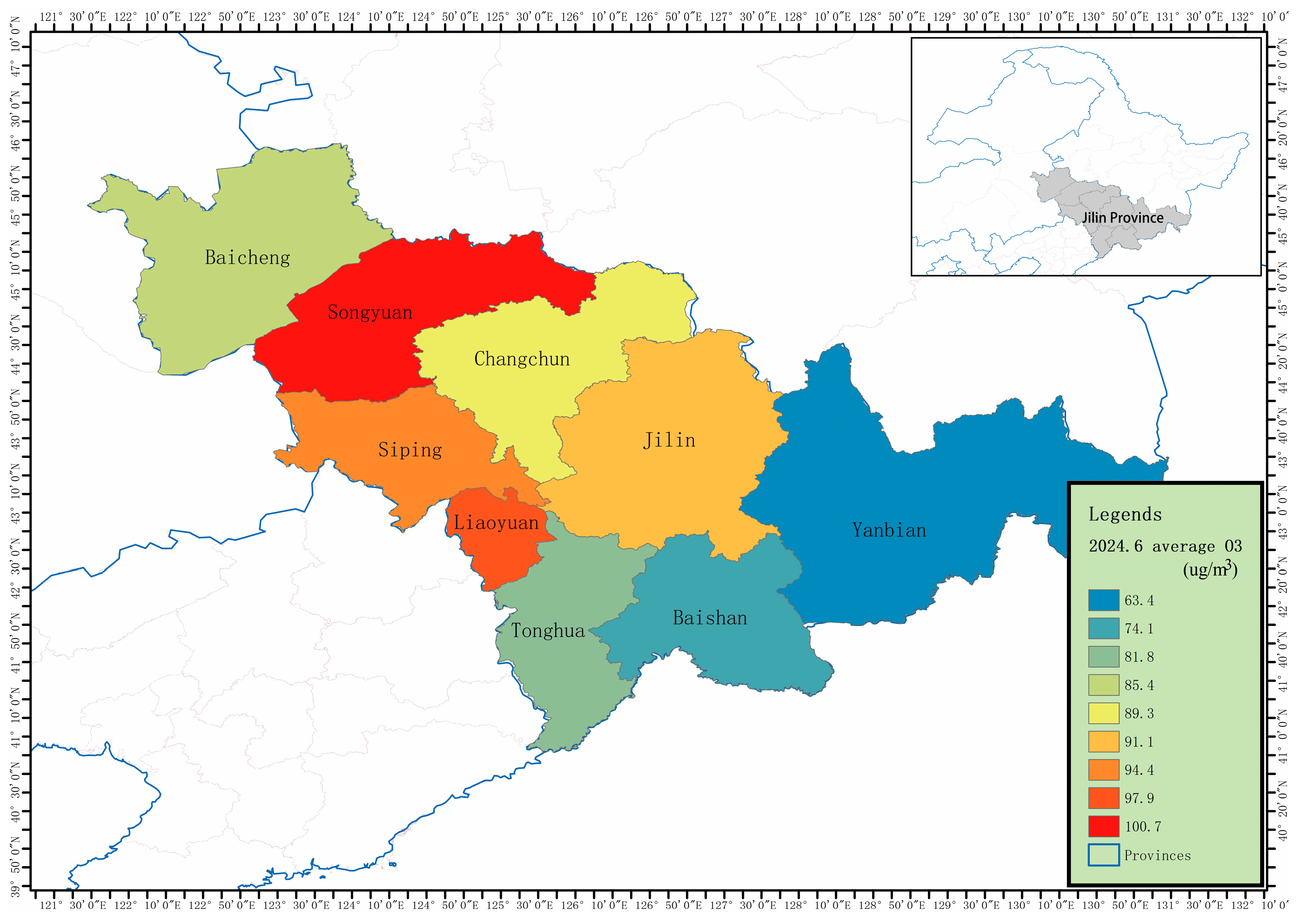
3.1.1. Analysis of Spatial Distribution Characteristics

Jilin Province comprises nine prefecture-level divisions: Changchun, Jilin, Siping, Liaoyuan, Tonghua, Baishan, Songyuan, Baicheng, and the Yanbian Korean Autonomous Prefecture. Figure 2 shows the ranking of the average O3 pollution concentrations in these nine regions for June 2024. As illustrated in this Figure, there are significant differences in the average O3 pollution concentrations among the regions in June. Spatially, the central and western parts of Jilin Province, such as Songyuan and Liaoyuan City, exhibit relatively higher pollution levels, while the eastern regions, including Yanbian Prefecture, show lower pollution levels. This reflects the spatial heterogeneity of O3 pollution across Jilin Province. Among the regions, Songyuan and Liaoyuan City have the highest pollution levels, whereas the Yanbian Korean Autonomous Prefecture has the lowest level.

3.1.2. Correlation Analysis with Meteorological Factors

To investigate the relationship between atmospheric pollutants and meteorological factors, Table 3 presents the correlations between the concentrations of six atmospheric pollutants in Liaoyuan City in 2024 and local temperature (T), pressure (P), and wind speed (WS). The degree of correlation is expressed using the Pearson correlation coefficient (r). The results indicate that O3 exhibits negative correlations with the concentrations of the other five pollutants [32], with the strongest negative correlation observed between O3 and NO2 (r = −0.54). As is well known, O3 is not a primary emitted pollutant; NO2 and VOCs are its key precursors, and they undergo nonlinear reactions [33], forming a cyclic chain reaction process under sunlight. Temperature shows a significant positive correlation with O3 concentration (r = 0.21) [34], consistent with most research findings, as solar radiation serves as an energy source, providing the necessary conditions for photochemical reactions [35]. As radiation intensity increases, the photochemical reaction process accelerates, increasing O3 concentrations [36]. Atmospheric pressure also shows a significant positive correlation with O3 concentration (r = 0.23), likely because high pressure brings stable meteorological conditions that promote photochemical reactions and O3 accumulation [34].

3.1.3. Annual Variation Characteristics of Pollution

According to the Technical Regulation on Ambient Air Quality Index (on trial) (HJ 633-2012), the proportions of the primary air pollutants in Liaoyuan City from 2021 to 2024 were calculated and are shown in Table 4. During this period, the primary pollutants only include O3, PM10, and PM2.5. Among them, PM10 is not always the primary pollutant each year, and it accounts for a relatively small proportion. The proportion of PM2.5 as the primary pollutant fluctuates over the four years. Meanwhile, the proportion of days with O3 as the primary air pollutant out of the total exceedance days shows a year-to-year increasing trend, increasing from 31.03% in 2021 to 52.60% in 2024. This indicates that O3 pollution became increasingly severe over those four years and requires our attention.

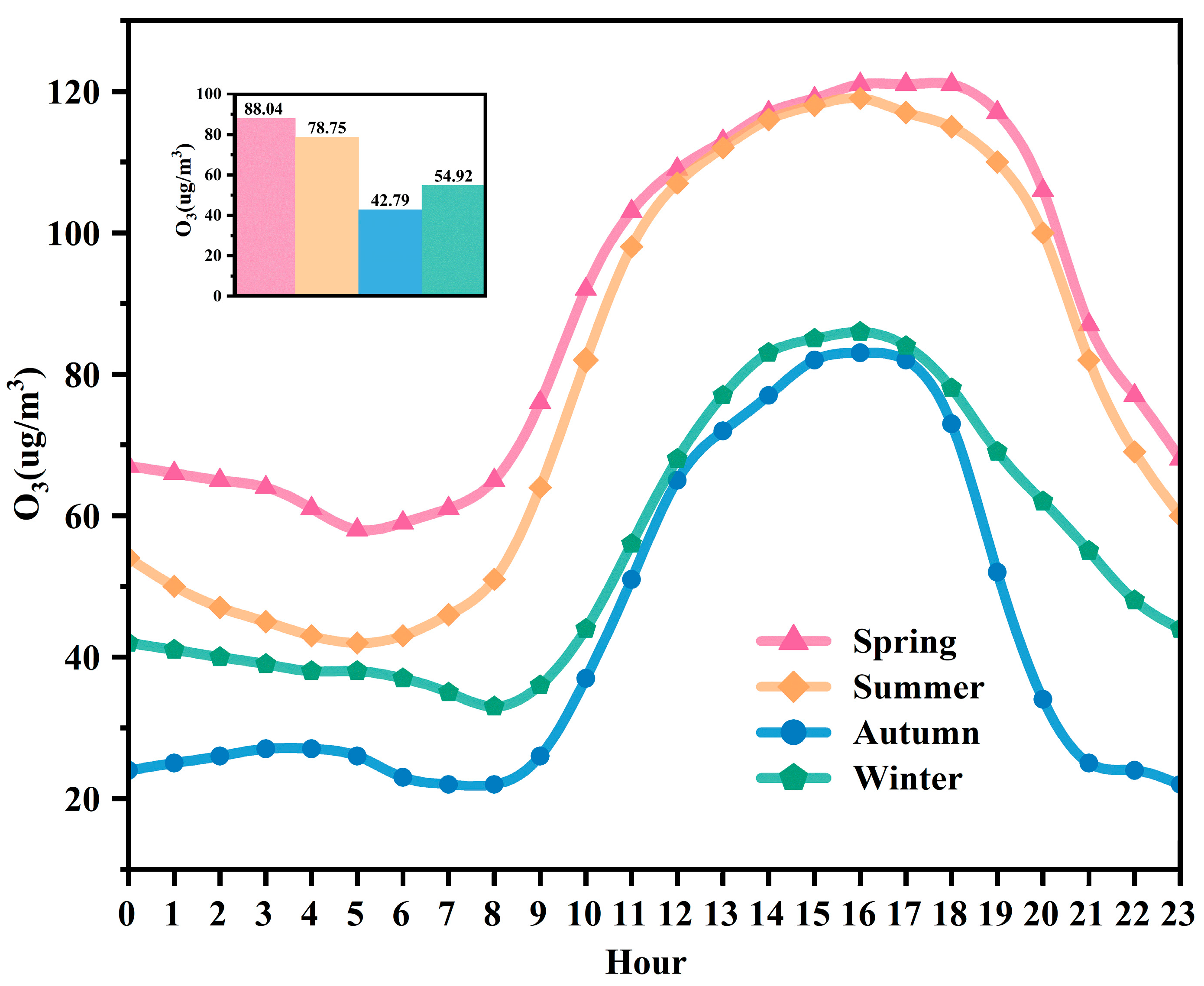
3.1.4. Seasonal Variation Characteristics of Pollution

Figure 3 illustrates the seasonal variation in the O3 concentrations in Liaoyuan City in 2024. Overall, the O3 concentrations exhibit significant seasonal differences, with the most severe pollution occurring in spring, followed by summer, while autumn and winter show notably lower pollution levels compared to the other seasons. The average concentration difference between spring and autumn is 45.25 μg/m3. The diurnal variation trend of O3 in each season follows a single-peak and single-valley pattern, with daily peaks occurring between 14:00 and 17:00. The daily low values occur between 4:00 and 6:00 in spring and summer and between 7:00 and 9:00 in autumn and winter. This pattern can be attributed to the titration effect of NO on O3 during the early morning hours [37], maintaining O3 concentrations at low levels. In the morning, the accumulated NO2 from the previous night and the NO emissions from sources such as motor vehicles during the morning rush hour remain at high concentrations [38]. As the boundary layer height rises and solar radiation intensity significantly increases, the O3 generation mechanism dominated by photolysis reactions is rapidly activated [39], causing O3 concentrations to continuously increase and reach their peak at around 14:00 to 17:00.

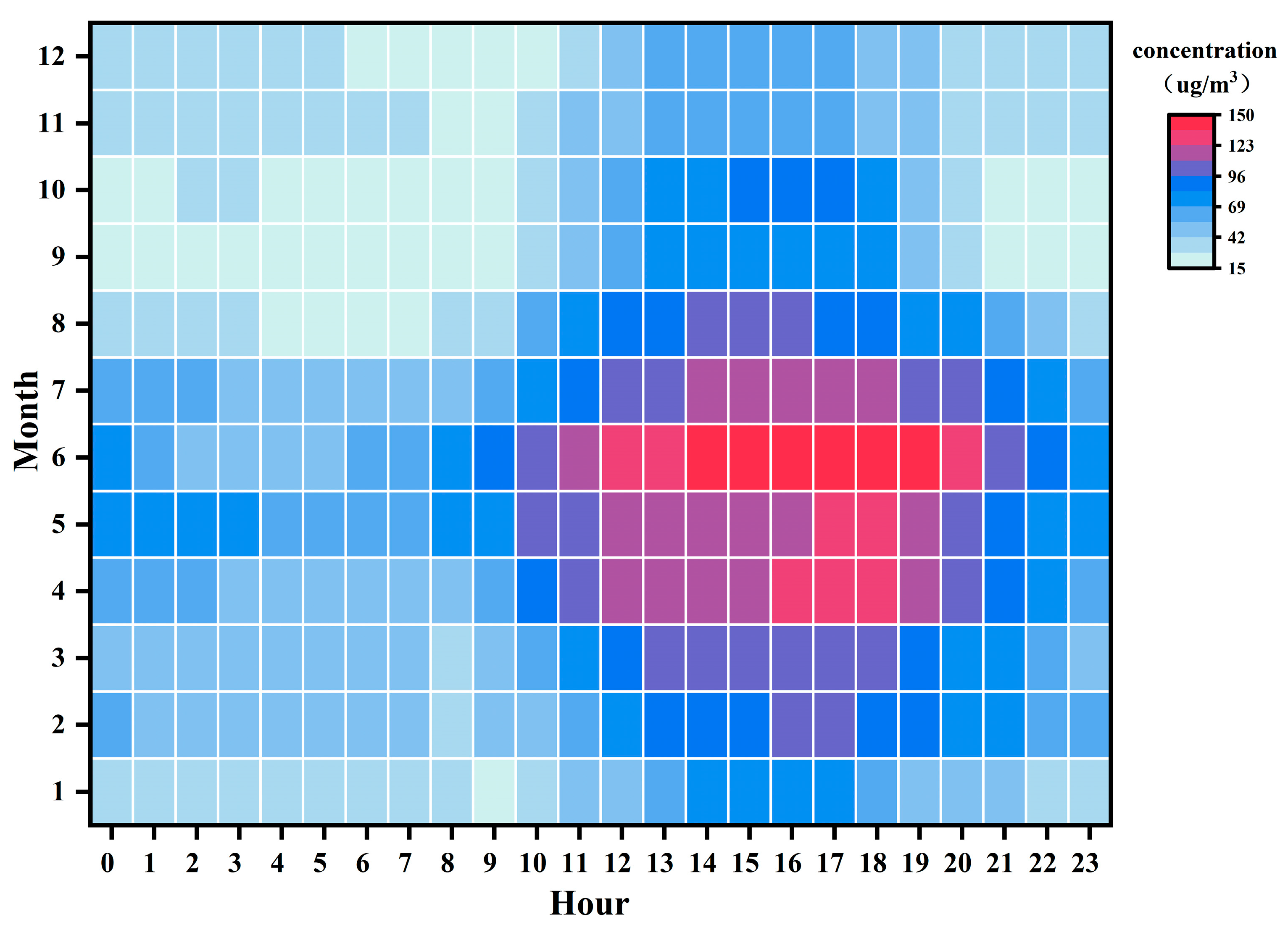
3.1.5. Monthly Variation Characteristics of Pollution

Figure 4 shows the monthly average O3 concentration changes in Liaoyuan City from 2015 to 2024. Overall, the O3 concentrations exhibited significant monthly fluctuations, with their peak values concentrated in May and June. The highest monthly average concentration in the past decade was recorded in June 2018 (117 μg/m3). This phenomenon is closely related to the meteorological conditions in late spring and early summer, where increased sunshine duration and enhanced solar radiation accelerate photochemical reactions, while stable atmospheric conditions hinder pollutant dispersion [40]. Notably, abnormally low values were observed in 2020 and 2021, primarily due to the reduced anthropogenic emissions of O3 precursors during the COVID-19 pandemic [41]. Figure 5 illustrates the monthly variation in the O3 concentrations in Liaoyuan City in 2024. Contrasting with recent years, the O3 concentrations are higher from April to July in the afternoon to early evening periods, corresponding to the spring and summer seasons, closely associated with strong sunlight and higher temperatures [34]. Among these months, June experienced the most severe O3 pollution.

3.2. Factors Affecting Ozone Concentrations

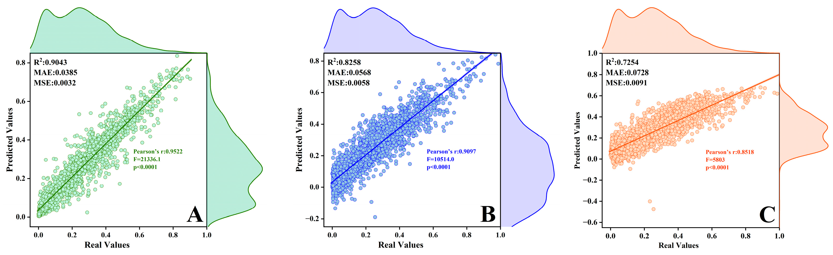
3.2.1. Comparative Study of Machine Learning Models

To thoroughly analyze the complex nonlinear relationships between the meteorological factors, non-meteorological factors, and O3 concentrations in Liaoyuan City, we decouple factors such as temporal variations, meteorological conditions, and pollution source emissions to investigate the specific contributions of these factors to O3 pollution. RF, ANN, and SVM, three models with strong nonlinear fitting capabilities, are selected for comparative study. The dataset used in this study covers hourly data for the entirety of 2024, divided into training and testing sets at a ratio of 3:1. Specifically, 6588 data points from 2024 are used for model training, while the remaining 2196 data points are used for model validation. To further improve computational efficiency, all data except temporal variables and wind direction are normalized before being input into the models. Additionally, the main parameters of the models are fine-tuned using a grid search method. The performances of the three models are comprehensively and accurately evaluated using metrics such as the coefficient of determination (R2), root mean square error (RMSE), and mean absolute error (MAE), combined with a five-fold cross-validation approach, to identify the best-performing parameterized model.
Figure 6 presents the regression plots of the predicted versus actual values for the following three models: RF, ANN, and SVM. The detailed process and the other result of ML are shown in Figures S1–S3. In terms of evaluation metrics, the RF model demonstrates superior performance, achieving the highest R2 value of 0.9043, indicating the strongest ability to explain data variability. Compared to the other two models, RF exhibits the best goodness of fit to the data as well. Additionally, its MAE of 0.0385 and RMSE of 0.0032 are the lowest among the three models, suggesting that the smallest deviation between the predicted and actual values and the highest prediction accuracy are recorded using this method. In contrast, both ANN and SVM produce negative predictions for O3 concentrations in some cases, and their R2 values are lower than those of the RF model. In reality, O3 concentrations cannot be negative, and these prediction results highlight the limitations of ANN and SVM in handling the dataset and making predictions in this case. At the same time, we also perform linear fitting on the real values and predicted values and conduct a significance test. The results indicate that random forest has the best fitting effect. Overall, among the three ML models compared, the RF model performed the best in terms of overall simulation effectiveness; therefore, it is more accurate in quantifying the relationships between meteorological factors, non-meteorological factors, and O3 concentrations.
Based on the RF model, a systematic assessment of the factors influencing the ground-level ozone in Liaoyuan City is conducted. Through feature importance analysis, the synergistic mechanisms of multi-source driving factors are revealed. As shown in Table 5, the top 15 key independent variables ranked by their contribution are as follows: NO2 > Second Quarter > Vegetation Coverage > Sea Surface Temperature > PM2.5 > Water Vapor Content > Latent Heat > Downward Shortwave Radiation > CO > 10 m Wind Speed > 2 m Specific Humidity > Sensible Heat Flux > Ground Heat Flux > Surface Longwave Radiation > Outgoing Longwave Radiation. The results indicate that O3 generation is jointly regulated by precursor concentrations, meteorological factors, and underlying surface characteristics, with significant nonlinear interactions among different factors [37,42]. Among these, NO2 exhibits a significantly higher contribution than the other variables, serving as the primary driving factor. This underscores the high sensitivity of O3 generation to precursors [43]. The high contribution of the second quarter (April, May, and June) aligns well with the monthly peak O3 concentrations in Liaoyuan City. During this period, increased solar radiation, elevated boundary layer height, and high temperatures significantly and collectively create an optimal environment for photochemical reactions [44,45]. These meteorological conditions favor the generation and accumulation of O3, leading to peak concentrations occurring during this time. The 10 m wind speed and specific humidity reflect the inhibitory effects of atmospheric diffusion capacity and humidity conditions on O3 accumulation. The indirect regulatory role of underlying surface characteristics is manifested through vegetation coverage and surface energy fluxes (sensible heat, latent heat). This association with vegetation coverage may stem from the dual effects of volatile organic compounds released by plants participating in photochemical reactions [46]. Notably, although the emission data of the main pollution sources serving as independent variables do not rank among the top 15, their fundamental influence on precursor concentrations remains existent [37]. The model results might be limited by the insufficient spatiotemporal resolution of the emission data or collinearity with other variables, which could explain their absence in the top rankings.

3.2.2. Analysis of Regional Transport

Using Liaoyuan City (42.77° N, 125.32° E) as the receptor point for backward trajectory simulation, that is at the black pentagram shown in Figure 7, the simulation period covers the entirety of 2024, with an initial height set at 100 m and a 48 h backward trajectory calculated at 1 h intervals, resulting in a total of 8784 trajectories. The trajectories are clustered into five average transport pathways using the NCAR meteorinfo software version 5.7, as shown in Figure 7. The other results of HYSPLIT clustering are shown in Figures S4–S8. The results indicate that trajectories 2, 4, and 5 exhibit spatial consistency, with a cumulative contribution rate of 45%. These trajectories are influenced by northwesterly airflows, which act as carriers for pollutant transport, continuously delivering pollutants from the regions along the trajectories to Liaoyuan City, thereby significantly impacting the city’s O3 pollution levels. Among these, trajectory 2 has the highest proportion (20%) and the shortest transport distance, indicating lower wind speeds. Source analysis reveals that this trajectory originates from the urban agglomeration in the central–western part of Jilin Province. Similarly, trajectory 3 also belongs to the short-distance, low-wind-speed transport type. The cumulative contribution rate of these two short-distance transport trajectories is 54%. During the transport process, due to the slower movement of air masses, O3 and its precursors, as well as other photochemical products, have more time to accumulate, leading to their continuous buildup during transport [47]. When these air masses arrive in Liaoyuan City, they interact and combine with pollutants generated from local industrial production, vehicle emissions, and agricultural activities, creating synergistic effects that provide the material basis for high O3 concentrations [37]. Additionally, specific meteorological conditions further exacerbate the severity of O3 pollution in Liaoyuan City.

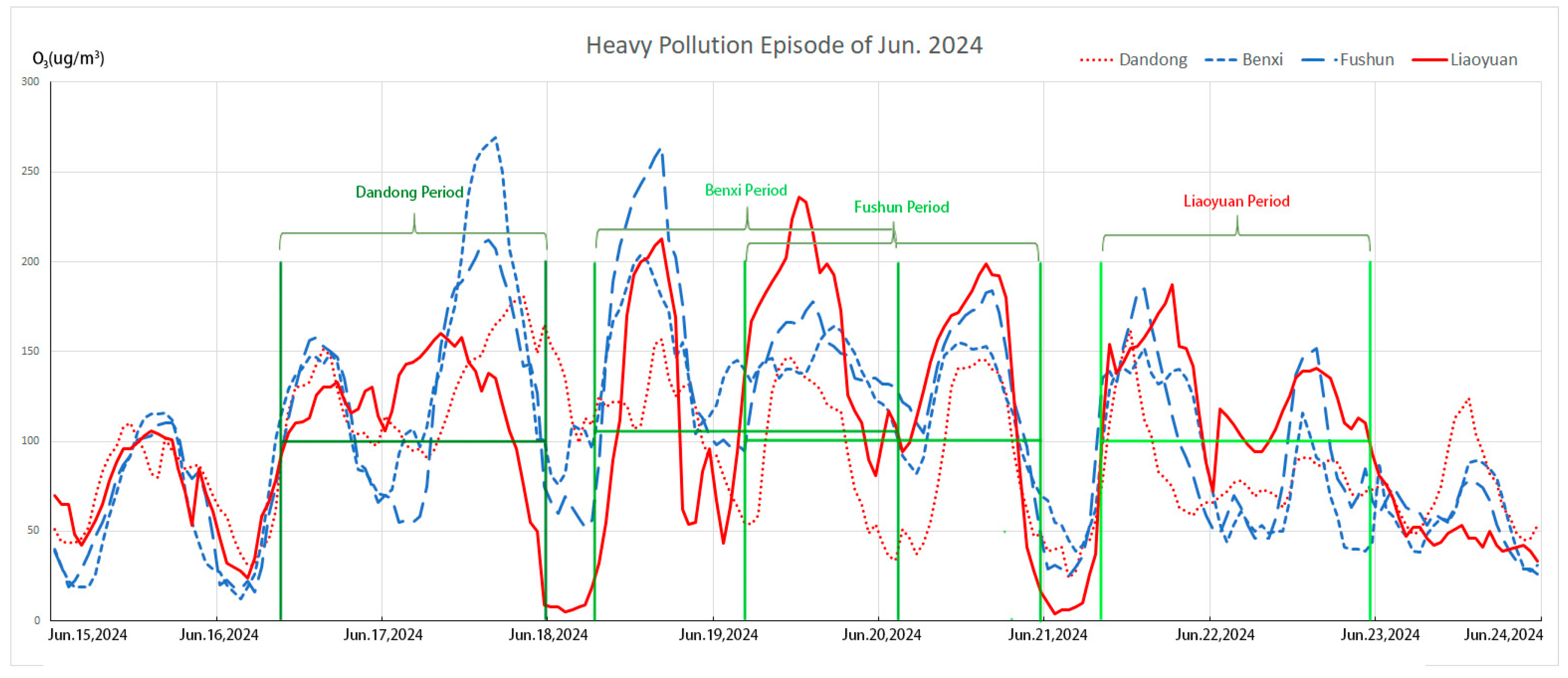
3.2.3. Analysis of Heavy Pollution Episodes

The monitoring data indicate that in June 2024, the proportion of days exceeding air quality standards in Liaoyuan City reached the highest level for the year, accounting for 36.7% of the month. Among these days, the number of days when O3 was identified as the primary pollutant was the highest. Therefore, this study selects a severe pollution period in mid-June (16–23 June) as the simulation period (we define this as more than 36 h of O3 heavy pollution even at night), as shown in Figure 8. Along path No. 3 in Figure 6 and path No. 2 in Figure 9, there is an obvious transportation route from the south to Liaoyuan City, which starts from East Sea, passing Dandong, Benxi City, and Fushun City. The Dandong period starts this heavy pollution episode in the morning on 16 June 2024, and the Liaoyuan period finishes the process at midnight on 23 June 2024. Relative research has found that a high O3 concentration will usually be accumulated in the mixed layer over the sea and will be transported to inland cities due to the land and sea breeze effect [48]. Thus, this should be the original source of this heavy pollution episode.
The backward trajectory clustering analysis is conducted to investigate the sources of pollution during heavy pollution days in Liaoyuan City, as illustrated in Figure 9. Using Liaoyuan City as the receptor site (the pentagram location in Figure 9, the backward trajectory simulations are initialized at an altitude of 100 m, with a time step of 1 h, and a total of 120 trajectories are obtained for a 48 h period. The cluster analysis identifies five major transport trajectories. Among them, trajectory 2 (28%) originates from the southwestern direction in Liaoning Province (Dandong–Benxi–Fushun region). Trajectory 3 (45%) originates from the eastern part of Shandong Province (Qingdao–Yantai region). Trajectory 4 (7%) originates from the southeast and has the longest transport distance. Collectively, these three transport pathways (trajectories 2, 3, and 4) account for 80% of the total, all covering maritime regions. The marine breeze facilitates the transfer of O3 from the oceanic atmosphere to the inland areas [48]. Simultaneously, these trajectories all traverse the central industrial belt of Liaoning Province [49], characterized by significant NOX and VOC pollution. Consequently, these factors collectively contribute to the elevated O3 concentrations observed in Liaoyuan City. The synergistic effects of transboundary pollution transport and local emissions significantly contribute to the O3 pollution episode, resulting in four consecutive days of exceedances in Liaoyuan City. During this period, the daily maximum increase in O3 concentration is 208 μg/m3, with a peak concentration of 236 μg/m3 recorded on June 19.

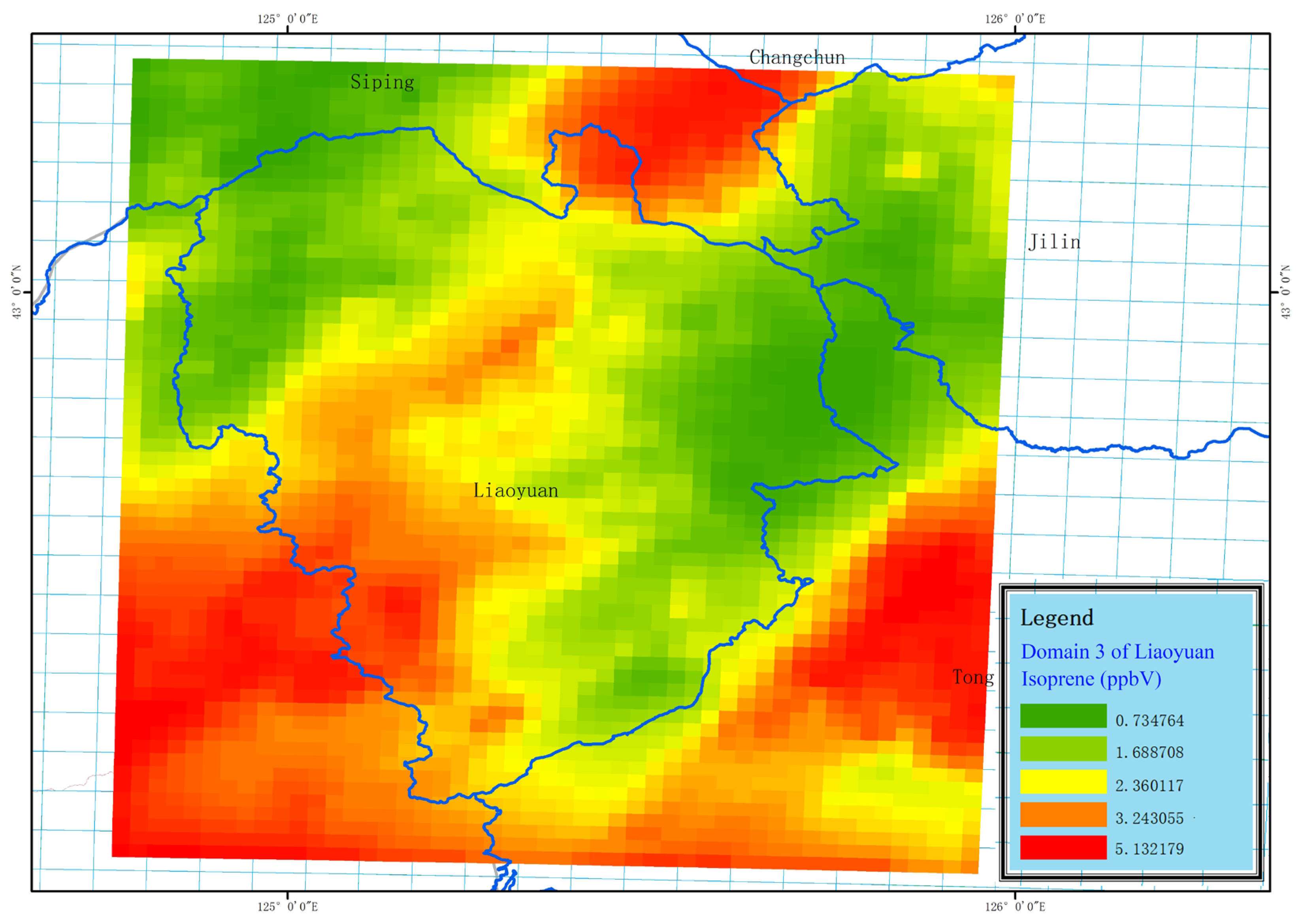
3.2.4. Analysis of Simulation of Air Pollution

To study the relationship between the O3 and VOCs in the atmosphere of Liaoyuan City, we conduct spatiotemporal simulations of O3, VOCs, and isoprene, and the results are shown in Figure 10 and Figure 11. Moreover, to evaluate the simulation effect of the CMAQ model, we selected the pollutant-monitoring stations 2227A and 2228A within the d03 (Figure 1) area of Liaoyuan City for verification and analysis. The model simulation O3 concentration data in the CMAQ grid where the pollutant monitoring stations are located are extracted and compared with the monitoring data of the corresponding stations. Following the reference standards proposed by Boylan et al. [50], in this paper, the verification indicator R of the simulation data and monitoring data of the CMAQ model is 0.63, the MFB is −0.11, and the MFE is 0.17. There exists a 32% underestimation of the simulation’s O3 concentration due to MEIC emission inventory without considering natural emission sources (MEGAN). The simulation results are excellent. The results show that during the severe pollution period in 2024, the concentrations of O3 and VOCs present a significant negative correlation, with a correlation coefficient of −0.47. The correlation coefficient between the concentrations of O3 and isoprene is 0.27, and the ratio of pollutant VOCs to NOx is 13.26, indicating that Liaoyuan City is in a VOC-controlling area.
Through the ISAM source apportionment module of CMAQ, we conduct a source analysis of the regional contribution of O3 during the heavy pollution periods in Liaoyuan City in 2024. The results are shown in Table 6. Among the nine prefecture-level divisions in Jilin Province, the contribution of Changchun City sources to its O3 is the highest, but the proportion is only 5.24%. The contribution of regions other than the nine prefecture-level divisions within d03 (Figure 1) is 30.40%. The contribution rate outside the domain 3 region is 44.05%, among which the contribution of the southern region is 40.06% and that of the northern region is only 3.99%. It is proven that about 95% of the O3 pollution in Liaoyuan City originates from regional transport.
This research confirms what many previous atmospheric O3 studies have already found regarding O3 formation in the summer season, O3 precursors, and sources. The analysis of pollution sources during the heavy pollution period suggests that the pollution episode in Liaoyuan City was primarily driven by the combined effects of regional transport, local emissions, and meteorological conditions. During this period, the prevailing wind direction was southwesterly. Additionally, mid-June coincided with the peak period of fertilizer and pesticide application, increasing emissions from agricultural activities that contributed to O3 exceedances [51]. Furthermore, continuous emissions of NOX from vehicle exhausts in urban areas exacerbated local pollution levels [52,53]. Unfavorable meteorological conditions, including strong solar radiation, high temperatures, and boundary layer compression, hindered pollutant dispersion and facilitated O3 accumulation [40]. These factors interacted, further deteriorating the air quality in Liaoyuan City and posing serious threats to urban environmental quality and public health [54].

4. Conclusions

Comparing the O3 pollution characteristics in Liaoyuan City with the surrounding cities, the O3 pollution in Liaoyuan City exhibits significant differences due to the influences of topography, industrial emissions, and variations in pollution control measures. The seasonal variation in O3 shows a high-value period from late spring to summer, characterized by a unimodal distribution peaking in May and June. This pattern is attributed to enhanced solar radiation and boundary layer elevation, which promote photochemical processes and drive O3 accumulation. In contrast, the lowest O3 concentrations occur in winter and early spring due to reduced photochemical reactivity under low temperatures. On a diurnal scale, O3 concentrations follow a distinct unimodal pattern, with peak values occurring in the afternoon, driven by the maximum intensity of solar radiation, which accelerates photolysis and facilitates the conversion of precursors into O3. Conversely, O3 concentrations remain low during the night-time and early morning, as nocturnal NO titration significantly reduces O3 levels.
A comparative analysis of three machine learning models indicates that the random forest model exhibits the best overall simulation performance, achieving an R2 value of 0.9043. Based on this model, this study comprehensively analyzes the factors influencing near-surface O3 concentrations in Liaoyuan City. The findings emphasize that precursor control remains the key strategy for mitigating O3 pollution, with a particular focus on the reduction in NOX emissions [55]. Additionally, meteorological factors and underlying surface characteristics also play crucial roles in O3 concentration variations [56]. These insights provide valuable guidance for future O3 pollution control strategies.
By using backward trajectory clustering analysis, the ISAM source apportionment module of CMAQ, and spatiotemporal simulations, we find that O3 pollution in Liaoyuan City is significantly influenced by regional transport and local sources; the main reasons for this include meteorology and precursors. This analytical result is completely consistent with the previous results in this paper. Therefore, in the control of O3 pollution in Liaoyuan City, joint prevention and control must be carried out, with particular attention paid to pollution control under the condition of southerly wind weather. This emphasizes the importance of regional collaboration in addressing O3 pollution.

Supplementary Materials

The following supporting information can be downloaded at https://www.mdpi.com/article/10.3390/toxics13060500/s1, Figure S1: Random Forest Model Simulation Result; Figure S2: Artificial Neural Network Model Simulation Result; Figure S3: Support Vector Machine Model Simulation Result; Figure S4: Clusters number’s TSV curve for 2024 whole year in Liaoyuan; Figure S5: 5-Cluster means curve for 2024 whole year in Liaoyuan; Figure S6: Clusters number’s TSV curve for June of 2024 in Liaoyuan; Figure S7: 5-Cluster means curve for June of 2024 in Liaoyuan; Figure S8: 5-Cluster trajectories for June of 2024 in Liaoyuan.

Author Contributions

Conceptualization, X.Z.; methodology, J.W.; validation, D.W. and J.W.; data curation, X.L.; writing—original draft preparation, X.Z.; writing—review and editing, D.W. and J.W.; supervision, J.W. All authors have read and agreed to the published version of the manuscript.

Funding

This research received no external funding.

Institutional Review Board Statement

Not applicable.

Informed Consent Statement

Not applicable.

Data Availability Statement

All the data generated or analyzed during this study are included in this manuscript and the Supplementary Files.

Conflicts of Interest

The authors declare no conflicts of interest.

References

  1. Li, K.; Jacob, D.J.; Liao, H.; Shen, L.; Zhang, Q.; Bates, K.H. Anthropogenic drivers of 2013–2017 trends in summer surface ozone in China. Proc. Natl. Acad. Sci. USA 2019, 116, 422–427. [Google Scholar] [CrossRef] [PubMed]
  2. Ahn, J.-W.; Dinh, T.-V.; Park, S.-Y.; Choi, I.-Y.; Park, C.-R.; Son, Y.-S. Characteristics of biogenic volatile organic compounds emit ted from major species of street trees and urban forests. Atmos. Pollut. Res. 2022, 13, 101470. [Google Scholar] [CrossRef]
  3. Oumami, S.; Arteta, J.; Guidard, V.; Tulet, P.; Hamer, P.D. Evaluation of Isoprene Emissions from the Coupled Model SURFEX-MEGANv2.1. EGUsphere 2023, 1–30. Available online: https://egusphere.copernicus.org/preprints/2023/egusphere-2023-2206/ (accessed on 11 June 2025). [CrossRef]
  4. Chen, Z.; Liu, J.; Cheng, X.; Yang, M.; Wang, H. Positive and negative influences of landfalling typhoons on tropospheric ozone over southern China. Atmos. Chem. Phys. 2021, 21, 16911–16923. [Google Scholar] [CrossRef]
  5. Pan, Q.; Harrou, F.; Sun, Y.J. A comparison of machine learning methods for ozone pollution prediction. J. Big Data 2023, 10, 63. [Google Scholar] [CrossRef]
  6. Cheng, Y.; He, L.Y.; Huang, X.F. Development of a high-performance machine learning model to predict ground ozone pollution in typical cities of China. J. Environ. Manag. 2021, 299, 113670. [Google Scholar] [CrossRef]
  7. Lu, H.; Xie, M.; Liu, X.; Liu, B.; Jiang, M.; Gao, Y.; Zhao, X. Adjusting prediction of ozone concentration based on CMAQ model and machine learning methods in Sichuan-Chongqing region, China. Atmos. Pollut. Res. 2021, 12, 101066. [Google Scholar] [CrossRef]
  8. Ma, R.; Ban, J.; Wang, Q.; Li, T. Statistical spatial-temporal modeling of ambient ozone exposure for environmental epidemiology studies: A review. Sci. Total Environ. 2020, 701, 134463. [Google Scholar] [CrossRef]
  9. Jumin, E.; Zaini, N.; Ahmed, A.N.; Abdullah, S.; Ismail, M.; Sherif, M.; Sefelnasr, A.; El-Shafie, A. Machine learning versus linear regression modelling approach for accurate ozone concentrations prediction. Eng. Appl. Comp. Fluid Mech. 2020, 14, 713–725. [Google Scholar] [CrossRef]
  10. Zhen, L.; Chen, B.; Wang, L.; Yang, L.; Xu, W.; Huang, R.-J. Data imbalance causes underestimation of high ozone pollution in machine learning models: A weighted support vector regression solution. Atmos. Environ. 2025, 343, 120952. [Google Scholar] [CrossRef]
  11. Yang, X.-T.; Kang, P.; Wang, A.-Y.; Zang, Z.-L.; Liu, L. Prediction of ozone pollution in Sichuan Basin based on random forest model. Environ. Sci. 2024, 45, 2507–2515. [Google Scholar] [CrossRef]
  12. Huang, Y.; Wang, Q.; Ou, X.; Sheng, D.; Yao, S.; Wu, C.; Wang, Q. Identification of response regulation governing ozone formation based on influential factors using a random forest approach. Heliyon 2024, 10, e36303. [Google Scholar] [CrossRef]
  13. Abdul Aziz, F.A.B.; Abd. Rahman, N.; Mohd Ali, J. Tropospheric Ozone Formation Estimation in Urban City, Bangi, Using Artificial Neural Network (ANN). Comput. Intell. Neurosci. 2019, 2019, 6252983. [Google Scholar] [CrossRef]
  14. Su, X.-Q.; An, J.-L.; Zhang, Y.-X.; Liang, J.-S.; Liu, J.-D.; Wang, X. Application of support vector machine regression in ozone forecasting. Huan Jing Ke Xue = Huanjing Kexue 2019, 40, 1697–1704. [Google Scholar] [CrossRef]
  15. Balogun, A.L.; Tella, A. Modelling and investigating the impacts of climatic variables on ozone concentration in Malaysia using correlation analysis with random forest, decision tree regression, linear regression, and support vector regression. Chemosphere 2022, 299, 134250. [Google Scholar] [CrossRef] [PubMed]
  16. Juarez, E.K.; Petersen, M.R. A Comparison of Machine Learning Methods to Forecast Tropospheric Ozone Levels in Delhi. Atmosphere 2022, 13, 46. [Google Scholar] [CrossRef]
  17. Luna, A.S.; Paredes, M.L.L.; De Oliveira, G.C.G.; Corrêa, S. Prediction of ozone concentration in tropospheric levels using artificial neural networks and support vector machine at Rio de Janeiro, Brazil. Atmos. Environ. 2014, 98, 98–104. [Google Scholar] [CrossRef]
  18. Lin, X.; Tong, J.-L.; Wang, Y.-F.; Chen, Y.-X.; Liu, Y.-L.; Zhang, X.; Ao, C.-J.; Liu, H.-T. Analysis of Causes and Sources of Summer Ozone Pollution in Rizhao Based on CMAQ and HYSPLIT Models. Huan Jing Ke Xue = Huanjing Kexue 2023, 44, 098–3107. [Google Scholar] [CrossRef]
  19. Zhang, K.; Xu, J.; Huang, Q.; Zhou, L.; Fu, Q.; Duan, Y.; Xiu, G. Precursors and potential sources of ground-level ozone in suburban Shanghai. Front. Environ. Sci. Eng. 2020, 14, 92. [Google Scholar] [CrossRef]
  20. Breiman, L. Random Forests. Mach. Learn. 2001, 45, 5–32. [Google Scholar] [CrossRef]
  21. Brokamp, C.; Rao, M.; Ryan, P.; Jandarov, R. A comparison of resampling and recursive partitioning methods in random forest for estimating the asymptotic variance using the infinitesimal jackknife. Stat 2017, 6, 360–372. [Google Scholar] [CrossRef]
  22. Halabaku, E.; Bytyçi, E. Overfitting in Machine Learning: A Comparative Analysis of Decision Trees and Random Forests. Intell. Autom. Soft. Comput. 2024, 39, 987–1006. [Google Scholar] [CrossRef]
  23. Lu, W.Z.; Wang, W.J. Potential assessment of the “support vector machine” method in forecasting ambient air pollutant trends. Chemosphere 2005, 59, 693–701. [Google Scholar] [CrossRef] [PubMed]
  24. Evgeniou, T.; Pontil, M. Machine Learning and Its Applications; Springer: Berlin/Heidelberg, Germany, 1999; pp. 249–257. [Google Scholar]
  25. Sewell, M. Structural Risk Minimization. Ph.D. Dissertation, Department of Computer Science, University College London, London, UK, 2008. [Google Scholar]
  26. Haykin, S. Neural Networks: A Comprehensive Foundation; Prentice Hall PTR: New Jersey, NJ, USA, 1994. [Google Scholar]
  27. Elharrouss, O.; Akbari, Y.; Almadeed, N.; Al-Maadeed, S. Backbones-review: Feature extractor networks for deep learning and deep reinforcement learning approaches in computer vision. Comput. Sci. Rev. 2024, 53, 100645. [Google Scholar] [CrossRef]
  28. Stein, A.F.; Draxler, R.R.; Rolph, G.D.; Stunder, B.J.B.; Cohen, M.D.; Ngan, F. NOAA’s HYSPLIT atmospheric transport and dispersion modeling system. Bull. Am. Meteorol. Soc. 2015, 96, 2059–2077. [Google Scholar] [CrossRef]
  29. Cui, L.; Song, X.; Zhong, G. Comparative analysis of three methods for HYSPLIT atmospheric trajectories clustering. Atmosphere 2021, 12, 698. [Google Scholar] [CrossRef]
  30. Skamarock, W.C.; Klemp, J.B.; Dudhia, J.; Gill, D.O.; Liu, Z.; Berner, J.; Wang, W.; Powers, J.G.; Duda, M.G.; Barker, D.M.; et al. A description of the advanced research WRF model version 4. Natl. Cent. Atmos. Res. 2019, 145, 550. [Google Scholar]
  31. Li, M.; Liu, H.; Geng, G.; Hong, C.; Liu, F.; Song, Y.; Tong, D.; Zheng, B.; Cui, H.; Man, H.; et al. Anthropogenic emission inventories in China: A review. Natl. Sci. Rev. 2017, 4, 834–866. [Google Scholar] [CrossRef]
  32. Yildizhan, H.; Udriștioiu, M.T.; Pekdogan, T.; Ameen, A. Observational study of ground-level ozone and climatic factors in Craiova, Romania, based on one-year high-resolution data. Sci. Rep. 2024, 14, 26733. [Google Scholar] [CrossRef]
  33. Chu, P.; Zhang, L.; Wang, Z.; Wei, L.; Liu, Y.; Dai, H.; Duan, E.; Deng, J. Synergistic catalytic elimination of NOX and VOCs: State of the art and open challenges. Surf. Interfaces 2024, 51, 104718. [Google Scholar] [CrossRef]
  34. Zhang, K.; Chen, Q.; Hong, Y.; Ji, X.; Chen, G.; Lin, Z.; Zhang, F.; Wu, Y.; Yi, Z.; Zhang, F.; et al. Elucidating contributions of meteorology and emissions to O3 variations in coastal city of China during 2019–2022: Insights from VOCs sources. Environ. Pollut. 2025, 366, 125491. [Google Scholar] [CrossRef] [PubMed]
  35. Li, Y.; Ye, C.; Ma, X.; Tan, Z.; Yang, X.; Zhai, T.; Liu, Y.; Lu, K.; Zhang, Y. Radical chemistry and VOCs-NOX-O3-nitrate sensitivity in the polluted atmosphere of a suburban site in the North China Plain. Sci. Total Environ. 2024, 947, 174405. [Google Scholar] [CrossRef] [PubMed]
  36. Yao, T.; Ye, H.; Wang, Y.; Zhang, J.; Guo, J.; Li, J. Kolmogorov-Zurbenko filter coupled with machine learning to reveal multiple drivers of surface ozone pollution in China from 2015 to 2022. Sci. Total Environ. 2024, 949, 175093. [Google Scholar] [CrossRef] [PubMed]
  37. Zhang, M.; Liu, Y.; Xu, X.; He, J.; Ji, D.; Qu, K.; Xu, Y.; Cong, C.; Wang, Y. A Systematic Review on Atmospheric Ozone Pollution in a Typical Peninsula Region of North China: Formation Mechanism, Spatiotemporal Distribution, Source Apportionment, and Health and Ecological Effects. Curr. Pollut. Rep. 2025, 11, 9. [Google Scholar] [CrossRef]
  38. de Souza, A.; de Oliveira-Júnior, J.F.; Cardoso, K.R.A.; Gautam, S. Impact of vehicular emissions on ozone levels: A comprehensive study of nitric oxide and ozone interactions in urban areas. Geosyst. Geoenviron. 2025, 4, 100348. [Google Scholar] [CrossRef]
  39. Wang, Z.; Zhang, H.; Shi, C.; Ji, X.; Zhu, Y.; Xia, C.; Sun, X.; Zhang, M.; Lin, X.; Yan, S.; et al. Vertical and spatial differences in ozone formation sensitivities under different ozone pollution levels in eastern Chinese cities. Npj Clim. Atmos. Sci. 2025, 8, 30. [Google Scholar] [CrossRef]
  40. Tong, Z.; Yan, Y.; Kong, S.; Niu, X.; Ma, J. Improving ozone estimation during rainy-warm seasons from the perspective of weather systems based on machine learning. Sci. Total Environ. 2025, 958, 177975. [Google Scholar] [CrossRef]
  41. Wang, D.; Pu, D.; De Smedt, I.; Zhu, L.; Yang, X.; Sun, W.; Xia, H.; Song, Z.; Li, X.; Li, J.; et al. Evolution of global O3-NOX-VOCs sensitivity before and after the COVID-19 from the ratio of formaldehyde to NO2 from satellites observations. J. Environ. Sci. 2024, 156, 102–113. [Google Scholar] [CrossRef]
  42. Wu, S.; Hou, L.; Sun, X.; Liu, M.; Wang, N.; Li, R. Characterizing temporal trends and meteorological influences on ozone pollution in Shenyang region (2018–2021). Air Qual. Atmos. Health 2025, 18, 1169–1182. [Google Scholar] [CrossRef]
  43. Chu, W.; Li, H.; Ji, Y.; Zhang, X.; Xue, L.; Gao, J.; An, C. Research on ozone formation sensitivity based on observational methods: Development history, methodology, and application and prospects in China. J. Environ. Sci. 2024, 138, 543–560. [Google Scholar] [CrossRef]
  44. Wang, Y.; Ding, D.; Kang, N.; Xu, Z.; Yuan, H.; Ji, X.; Dou, Y.; Guo, L.; Shu, M.; Wang, X. Effects of combined exposure to PM2.5, O3, and NO2 on health risks of different disease populations in the Beijing-Tianjin-Hebei region. Sci. Total Environ. 2025, 958, 178103. [Google Scholar] [CrossRef] [PubMed]
  45. Wang, L.; Wan, B.; Yang, Y.; Fan, S.; Jing, Y.; Cheng, X.; Gao, Z.; Miao, S.; Zou, H. Atmospheric Boundary Layer Stability in Urban Beijing: Insights from Meteorological Tower and Doppler Wind Lidar. Remote Sens. 2024, 16, 4246. [Google Scholar] [CrossRef]
  46. Li, M.; Wang, R. Combined Catalytic Conversion of NOX and VOCs: Present Status and Prospects. Materials 2024, 18, 39. [Google Scholar] [CrossRef]
  47. Wang, C.; Li, J.; An, X.; Liu, Z.; Zhang, D. Sensitivity analysis and precursor emission sources reduction strategies of O3 for different pollution weather types based on the GRAPES-CUACE adjoint model. Atmos. Environ. 2024, 333, 120632. [Google Scholar] [CrossRef]
  48. Zhao, D.; Xin, J.; Wang, W.; Jia, D.; Wang, Z.; Xiao, H.; Liu, C.; Zhou, J.; Tong, L.; Ma, Y.; et al. Effects of the sea-land breeze on coastal ozone pollution in the Yangtze River Delta, China. Sci. Total Environ. 2022, 807, 150306. [Google Scholar] [CrossRef]
  49. Ma, L. Decomposition of China’s industrial environment pollution change based on LMDI. Geogr. Res. 2016, 35, 1857–1868. [Google Scholar]
  50. Boylan, J.W.; Russell, A.G. PM and light extinction model performance metrics, goals, and criteria for three-dimensional air quality models. Atmos. Environ. 2006, 40, 4946–4959. [Google Scholar] [CrossRef]
  51. Du, C.; Pei, J.; Feng, Z.J. Unraveling the complex interactions between ozone pollution and agricultural productivity in China’s main winter wheat region using an interpretable machine learning framework. Sci. Total Environ. 2024, 954, 176293. [Google Scholar] [CrossRef]
  52. Zheng, B.; Tong, D.; Li, M.; Liu, F.; Hong, C.; Geng, G.; Li, H.; Li, X.; Peng, L.; Qi, J.; et al. Trends in China’s anthropogenic emissions since 2010 as the consequence of clean air actions. Atmos. Chem. Phys. 2018, 18, 14095–14111. [Google Scholar] [CrossRef]
  53. Li, M.; Huang, X.; Yan, D.; Lai, S.; Zhang, Z.; Zhu, L.; Lu, Y.; Jiang, X.; Wang, N.; Wang, T.; et al. Coping with the concurrent heatwaves and ozone extremes in China under a warming climate. Sci. Bull. 2024, 69, 2938–2947. [Google Scholar] [CrossRef]
  54. Brown, J.; Bowman, C. Integrated Science Assessment for Ozone and Related Photochemical Oxidants; US Environmental Protection Agency: Washington, DC, USA, 2013.
  55. Cao, X.C.; Wu, X.C.; Xu, W.S.; Xie, R.; Xian, A.; Yang, Z. Pollution characterization, ozone formation potential and source apportionment of ambient VOCs in Sanya, China. Res. Environ. Sci. 2021, 34, 1812–1824. [Google Scholar]
  56. Wang, M.; Zheng, Y.F.; Liu, Y.J.; Li, Q.P.; Ding, Y.H. Characteristics of ozone and its relationship with meteorological factors in Beijing-Tianjin-Hebei Region. China Environ. Sci. 2019, 39, 2689–2698. [Google Scholar]
Figure 1. Three-layer nested map for WRF simulation.
Toxics 13 00500 g001
Figure 2. Geographic location of Jilin Province and ranking of average O3 pollution concentrations in June 2024.
Toxics 13 00500 g002
Figure 3. Daily variations in O3 concentrations in different seasons for 2024.
Toxics 13 00500 g003
Figure 4. Monthly variations in O3 concentrations in Liaoyuan City from 2015 to 2024.
Toxics 13 00500 g004
Figure 5. Hourly variations in O3 concentrations in different months for 2024.
Toxics 13 00500 g005
Figure 6. Regression fitting lines for O3 concentration using three machine learning methods in Liaoyuan City: (A) RF, (B) ANN, and (C) SVM.
Toxics 13 00500 g006
Figure 7. Backward trajectory clustering analysis in 2024.
Toxics 13 00500 g007
Figure 8. Period analysis of O3 heavy pollution episode in 2024.
Toxics 13 00500 g008
Figure 9. Backward trajectory clustering analysis of heavy pollution episode in 2024.
Toxics 13 00500 g009
Figure 10. The simulation and verification results of air pollution during the heavy pollution episodes in Liaoyuan City in 2024.
Toxics 13 00500 g010
Figure 11. The spatial distribution of isoprene in Liaoyuan City during the heavy pollution episodes in 2024.
Toxics 13 00500 g011
Table 1. Parameterization scheme settings for WRF simulation.
ParametersSettings
Microphysical Process SchemeThompson
Short-wave Radiation SchemeRapid Radiative Transfer Model
Long-wave Radiation SchemeRapid Radiative Transfer Model
Land surface Process SchemeNoah Land Surface Model
Boundary Layer SchemeYSU (Yonsei University)
Cumulus Parametric SchemeKain–Fritsch (New Eta)
Table 2. Formulas for evaluation indicators.
IndicatorsFormulas
MFB 1 N i = 1 N m i O i O i + m i 2
MFE 1 N i = 1 N m i O i O i + m i 2
R i = 1 N m i m ¯ O i O ¯ i = 1 N m i m ¯ 2 i = 1 N O i O ¯ 2
Table 3. Correlations between pollutants and meteorological factors in Liaoyuan City for 2024.
VariablesPM2.5PM10SO2NO2O3COTPWS
PM2.51.000
PM100.900 **1.000
SO20.440 **0.380 **1.000
NO20.470 **0.410 **0.290 **1.000
O3−0.170 **−0.160 **−0.071 **−0.540 **1.000
CO0.630 **0.530 **0.260 **0.630 **−0.350 **1.000
T−0.300 **−0.270 **−0.260 **−0.260 **0.210 **−0.230 **1.000
P−0.340 **−0.310 **−0.300 **−0.290 **0.230 **−0.220 **0.920 **1.000
WS−0.0280.0093−0.030−0.090 **0.059 **−0.099 **0.240 **0.00281.000
** p < 0.01.
Table 4. Proportion of primary pollutants in Liaoyuan City from 2021 to 2024.
YearPM2.5 (%)PM10 (%)O3 (%)
202165.523.4531.03
202251.300.0048.70
202339.1010.9050.00
202442.105.3052.60
Table 5. Feature importance ranking in the RF model.
IDVariablesCategoriesValue
1NO2Monitoring Pollutants 0.6579
2Second QuarterTemporal Variables 0.1105
3Vegetation CoverageMeteorological Variables 0.0598
4Sea Surface TemperatureMeteorological Variables0.0550
5PM2.5Monitoring Pollutants 0.0458
6Water Vapor ContentMeteorological Variables0.0399
7Latent HeatMeteorological Variables0.0394
8Downward Shortwave RadiationMeteorological Variables0.0355
9COMonitoring Pollutants 0.0354
1010 m Wind SpeedMeteorological Variables0.0301
112 m Specific HumidityMeteorological Variables0.0256
12Sensible Heat FluxMeteorological Variables0.0145
13Ground Heat FluxMeteorological Variables0.0118
14Surface Longwave RadiationMeteorological Variables0.0089
15Outgoing Longwave RadiationMeteorological Variables0.0087
Table 6. ISAM result for Liaoyuan City in June 2024.
AreaContribution Concentration
(ug/m3)
Ratio (%)
Baicheng City2.01.44
Baishan City0.30.24
Changchun City7.25.24
Jilin City4.93.57
Liaoyuan City7.05.05
Siping City6.84.89
Songyuan City3.02.15
Tonghua City3.62.59
Yanbian0.50.37
Southeast Area to domain 318.213.15
Southwest Plain Area to domain 312.69.10
Southwest Mountain Area to domain 324.617.81
North Area to domain 35.53.99
Other Area in domain 342.030.40
Disclaimer/Publisher’s Note: The statements, opinions and data contained in all publications are solely those of the individual author(s) and contributor(s) and not of MDPI and/or the editor(s). MDPI and/or the editor(s) disclaim responsibility for any injury to people or property resulting from any ideas, methods, instructions or products referred to in the content.

