Abstract
Background: Disruptions in freight transportation—such as service delays, infrastructure failures, and labor strikes—pose significant challenges to the reliability and efficiency of intermodal networks. To address these challenges, this study introduces Adaptive Intermodal Transportation (AIT), a resilient and flexible planning framework that enhances Synchromodal Freight Transport (SFT) by integrating real-time disruption management. Methods: Building on recent advances, we propose two novel strategies: (1) Reassign with Delay Buffer, which enables dynamic rerouting of shipments within a user-defined delay tolerance, and (2) (De)Consolidation, which allows splitting or merging of shipments across services depending on available capacity. These strategies are incorporated into a re-planning module that complements a baseline optimization model and a continuous disruption-monitoring system. Numerical experiments conducted on a Great Lakes-based case study evaluate the performance of the proposed strategies against a benchmark approach. Results: Results show that under moderate and high-disruption conditions, the proposed strategies reduce delay and disruption-incurred costs while increasing the percentage of matched shipments. The Reassign with Delay Buffer strategy offers controlled flexibility, while (De)Consolidation improves resource utilization in constrained environments. Conclusions: Overall, the AIT framework demonstrates strong potential for improving operational resilience in intermodal freight systems by enabling adaptive, disruption-aware planning decisions.
1. Introduction
The transportation industry is the backbone of the economy, heavily relying on road transportation due to its flexibility, versatility, and accessibility. However, this unimodal dominance has significant drawbacks, including air pollution, congestion, and greenhouse gas (GHG) emissions, which are rising without any sign of reduction [1]. Freight transportation faces similar externalities, demanding efforts toward sustainability [2]. As a result, four main strategies for “Green Freight Transportation” have been introduced to alleviate these externalities: (1) reducing demand; (2) improving vehicle efficiency and transportation systems; (3) reducing carbon content in fuel; and (4) shifting freight to low-carbon modes such as rail and inland waterways [3]. Among these, modal shift approaches, particularly Synchromodal Freight Transport (SFT), have gained significant attention for their promise of combining sustainability with real-time, multi-modal flexibility [4].
SFT represents a dynamic and integrated network perspective, wherein multiple transportation modes such as road, rail, and waterways are used flexibly in response to changing conditions, fostering economic efficiency and environmental benefits [5]. By integrating real-time information sharing among stakeholders, SFT aims to synchronize transport modes dynamically, adapting to both supply and demand in an efficient manner [6]. Despite its potential, SFT remains vulnerable to disruptions. These may include service delays, infrastructure failures, labor strikes, cyber attacks, and demand fluctuations [7,8]. Although SFT is promising for integrated, flexible operations, this paper emphasizes resiliency under disruption. We therefore adopt the concept of Adaptive Intermodal Transportation (AIT) as an evolution of synchromodality, focused on dynamic re-planning and robust handling of real-world uncertainties and disruptions. More precisely, AIT builds upon the core principles of SFT by retaining its multimodal flexibility while explicitly incorporating real-time disruption management. Unlike traditional SFT, which focuses on dynamic mode coordination under nominal conditions, AIT introduces proactive re-planning strategies to enhance network resilience under uncertainty.
Disruptions in freight transportation introduce significant uncertainty into operational planning. These disruptions can lead to increased costs, delays, and even infeasible plans if not addressed promptly [9]. Such disruptions can jeopardize the reliability and effectiveness of transportation plans, highlighting the critical need for robust disruption-management mechanisms within the SFT framework. While traditional transportation models may rely on static plans, AIT’s real-time flexibility allows it to dynamically adjust plans, reroute shipments, and select alternative modes in response to real-time disruptions. This capability is vital to ensure that SFT remains resilient and reliable in the face of operational uncertainties [7].
Therefore, addressing these disruptions within AIT networks requires a decision-making framework that can handle unexpected disruptions. In order to effectively address transportation disruptions, it is crucial to detect unforeseen events that could cause disruptions and evaluate their potential impact on the logistics network. Recent developments on re-planning strategy for AIT transportation [10,11] swiftly provide alternative solutions, which is essential in minimizing disruption-related consequences. Efficient re-planning of SFT in response to disruptions requires seamless integration of planning, execution, and continuous monitoring of transportation activities to ensure optimal results [12]. The study presented here is built upon the framework by [8,10,11] to adapt and advance their current state of disruption handling. This study contributes to the growing body of SFT literature by introducing new disruption-handling strategies:
- Introduction of a novel “Reassign with Delay Buffer” strategy that facilitates a more dynamic response to service delays. This approach allows the decision-makers to adjust the conservativeness level of the disruption response based on specific operational needs. By incorporating flexibility into the delay buffer, the model accommodates various scenarios, giving stakeholders the ability to tailor the response strategy in line with their risk tolerance and urgency requirements.
- The formulation of a unique (De)Consolidation re-planning approach specifically designed for disrupted shipments. To the best of our knowledge, this is the first time a consolidation and deconsolidation mechanism has been explicitly integrated into a disruption-response framework. This approach enables the model to determine the optimal course of action for each affected shipment request, considering whether to consolidate shipments into fewer services or deconsolidate them across multiple services based on the available capacity and service constraints.
The adapted framework in this study consists of three key modules: an offline (baseline) planning module, a disruption-monitoring module, and an online (re-planning) module with the new strategies.
The offline (baseline) planning module, based on the previous work of the authors [8,13], is responsible for generating plans to serve the demand, under the assumption of a deterministic environment where no disruptions are anticipated. This baseline plan establishes an optimal transportation strategy based solely on static conditions, enabling the system to function efficiently in the absence of unforeseen events.
The disruption-monitoring module, an extension to the current framework developed in [10,11], operates continuously to track potential disruptions in service and demand, considering expanded disruption and delay types that are introduced and used in this paper. When a disruption occurs, this module assesses its impact by updating information across the service, demand, and infrastructure dimensions. By assessing the impact of disruptions, this module ensures that the system remains aware of changes that may affect the transportation plan.
The online (re-planning) module advances the current work in [10,11] by employing two new strategies of “Reassign with Delay Buffer”, and “(De)Consolidation” in addition to the benchmark strategy of “Always Wait”. Each strategy offers a unique approach to handling disruptions: the benchmark “Always Wait” strategy maintains the existing schedule, allowing for delays as services wait for disruptions to clear, the new “Reassign with Delay Buffer” strategy reallocates shipments to alternative routes or schedules, allowing for flexible adjustments within a predefined delay tolerance, and the new “(De)Consolidation” strategy enables the system to split or combine shipments, optimizing capacity and ensuring continuity despite disruptions.
These three modules are interconnected, allowing the methodology to deliver a coordinated, reactive response to disruptions to ensure that transportation plans remain resilient and adaptable in the face of dynamic operational challenges.
In summary, this study proposes a modular adaptive intermodal transportation framework that incorporates two new disruption-handling strategies, namely Reassign with Delay Buffer and (De)Consolidation. The framework advances the literature by explicitly addressing disruption management and offers practical value by enhancing the resilience and flexibility of freight transportation networks under uncertainty.
The remainder of this paper is structured as follows: Section 2 reviews the related literature on AIT transport and disruption management. Section 3 outlines the problem description, followed by the methodology in Section 4. Section 5 presents the results of the numerical experiments, providing insights into disruption-management strategies. Finally, Section 6 concludes with potential future research directions.
2. Literature Review
The concept of SFT and AIT freight transportation has been extensively explored in the literature from various angles, including service network design, shipment matching, and the physical internet—a next-generation extension of synchromodal networks. From a technical standpoint, synchromodal transportation has been modeled and analyzed using a variety of approaches. Optimization models have been commonly employed to address challenges in service scheduling, resource allocation, and cost minimization [8,14,15,16,17,18]. Additionally, reinforcement learning models have been applied to enhance decision-making processes in dynamic and uncertain environments, where adaptive learning can improve the efficiency of transportation networks [10,19,20]. Simulation models have also been used to capture the complexities of SFT and AIT systems, providing a virtual testing environment to evaluate different operational strategies [21,22,23,24,25].
Comprehensive reviews of these topics have been conducted by [4,26,27], which cover the advancements and the remaining gaps in AIT transportation research. Despite these studies, the role of disruption management within operational AIT planning remains an underexplored area. This gap is critical, as disruptions can significantly impact the robustness and reliability of AIT systems. The following section reviews the existing literature on disruption-management strategies that have been integrated into SFT frameworks, highlighting research gaps and the need for further exploration in this domain.
Most studies on disruption management in SFT focus on re-planning and dynamically adjusting baseline plans to accommodate disruptions. The primary distinctions among these studies arise from the specific strategies they implement to respond to disruptions and the types and range of disruptions that they can handle. For example, Van Riessen et al. [28] examined the effects of disruptions on rail and barge networks, proposing a framework to assess whether a service should be canceled based on the evaluated impact. In a similar vein, Qu et al. [29] developed a Mixed-Integer Linear Programming (MILP) model to re-plan hinterland SFT by leveraging detour options, shipment splitting (deconsolidation), and transshipment strategies as adaptive responses to disruptions.
In the context of port-hinterland container logistics, Hrušovskỳ et al. [7] proposed a real-time decision-support system for intermodal transportation networks. This system combines optimization and simulation techniques to assess disruption impacts and incorporates multiple strategies for re-planning, including “Always Wait”, “Transshipment”, and “Detour”. Additionally, Gao and Liu [30] introduced a bi-level programming model aimed at enhancing resiliency. The model’s upper level focuses on governmental decision-making for immediate recovery actions, while the lower level enables trucking carriers to make optimized decisions regarding routes and freight volumes. Furthermore, Karam and Reinau [31] presented a model integrating simulation, optimization, and cost-effectiveness analysis specifically for road freight, with applications in urban distribution systems. Their work emphasizes the importance of coordinated logistics in response to disruption events. Durán-Micco et al. [32] expanded on these concepts by employing an agent-based simulation model to evaluate the resiliency of freight networks under disruption. Their model re-plans routes and dynamically reroutes affected shipments, demonstrating the potential of simulation approaches to provide robust responses to unanticipated events. Dewantara [10] utilizes a hybrid discrete-event simulation-optimization modeling approach to assess the impact of disruptions and generate optimal response strategies. Additionally, a reinforcement learning agent is trained to select the most suitable strategy for each disruption, choosing between two primary options: Always Wait and Always Reassign.
Studies on disruption management in transportation and supply chains can also be categorized based on how they approach the analysis of disruption impacts. A significant portion of existing literature focuses predominantly on how disruptions affect service-related attributes, such as service time and service capacity reduction [10,14,32,33,34,35,36,37,38,39,40]. While these aspects are crucial, they only capture a part of the disruption’s influence on transportation networks. However, it is equally important to address the broader implications of disruptions on infrastructure, particularly on critical nodes such as container terminals and other intermodal facilities. Disruptions impacting such infrastructure can have cascading effects on the overall network by altering operational features essential for efficient transport, such as loading and unloading times, container-handling efficiency, and berth availability. When these operational capabilities are compromised due to a disruption, the affected node cannot function at its regular capacity, which directly impacts the flow of cargo. Despite the importance of studying these infrastructure-related impacts, relatively few studies have thoroughly examined them. Most research tends to overlook the effect of disruptions on the physical infrastructure and the subsequent operational and demand-related consequences [7,29,41,42,43]. Addressing this gap in future research could provide a more comprehensive understanding of disruption impacts and inform more resilient disruption-management strategies.
To the best of our knowledge, the research most closely related to the current study is the work of [10] and Hrušovskỳ et al. [7]. In the first study, Dewantara [10] developed a novel simulation-optimization model for synchromodal transportation as an environment to train a reinforcement learning agent, which aids in selecting the appropriate response to disruptions. Their approach incorporated two main disruption-handling strategies within the optimization model: “Always Wait” and “Always Reassign.” However, while effective as a baseline, these two strategies are limited in their adaptability. The “Always Wait” strategy results in costly delays when the disruption persists, while the “Always Reassign” policy lacks flexibility to consider varying levels of service delays. Our study extends this work by introducing additional strategies—namely, the delay buffer and (De)Consolidation strategies—which provide more granular control over the disruption response and enable better optimization of time and cost within synchromodal networks.
In the second study, Hrušovskỳ et al. [7] proposed a disruption-management framework that focused on re-planning strategies, specifically “Always Wait”, “Transshipment”, and “Reassign”. While their approach effectively demonstrates the importance of re-planning within a synchromodal context, it primarily leverages the inherent flexibility of the synchromodal system where transshipment is a readily available option for rerouting freight. In contrast, our study introduces a delay buffer policy that prepares for delays by allocating extra time in the planning phase, thus enhancing the resilience of the network against unforeseen disruptions. Additionally, the (De)Consolidation strategy in our model allows for adjusting the shipment load dynamically, which is particularly valuable in high-disruption scenarios, as it facilitates more efficient resource allocation across services without solely relying on transshipment.
In contrast, the current research introduces the “Reassign with Delay Buffer” strategy, which enhances disruption management by allowing for more dynamic and flexible decision-making. This delay buffer integrates a temporal margin into the reassignment process, offering decision-makers the ability to handle disruptions with a clearer understanding of potential delays. By incorporating this buffer, the framework becomes more adaptable to real-time uncertainties and provides more transparency and explanation behind the decisions made during disruption recovery. Moreover, this study introduces the new concept of Adaptive Intermodal Transportation (AIT), which is solely focused on enhancing the resiliency of synchromodal networks by prioritizing robust and flexible disruption management.
The other key contribution of this research is the introduction of the (De)Consolidation disruption-handling strategy. To the best of our knowledge, this is the first study in the field to implement such a strategy within the context of freight transportation. The (De)Consolidation strategy enables the model to either combine multiple shipment requests (consolidation) when service limitations exist or split a shipment into multiple services (deconsolidation) when no single service has sufficient capacity to accommodate the entire request. This approach is particularly useful when services face varying capacity constraints, allowing for a more efficient allocation of resources. By offering a structured methodology for both consolidation and deconsolidation, this research contributes to filling a critical gap in the literature on freight transportation disruption management.
3. Problem Description
To implement the AIT concept, this study employs a mode-free booking approach, based on the prior work of the authors [8,13,44]. The mode-free booking is managed by a centralized AIT operator, whereby cargo owners delegate the decision-making regarding transportation mode(s) to the operator based on its comprehensive network preferences. The platform receives shipment request details from cargo owners on the demand side, while service information is supplied by service providers on the supply side. Specifically, shipment request data includes the origin, destination, volume, due time, and release time, while the service data encompasses the origin, destination, capacity, departure time, arrival time, transportation mode, and service cost. As illustrated in Figure 1, the platform integrates supply, demand, and infrastructure elements to minimize the overall transportation utility while considering disruptions.
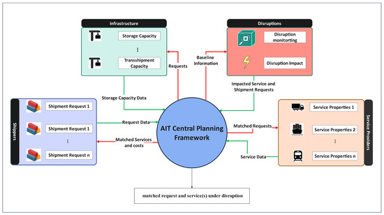
Figure 1.
General overview of the AIT global platform.
Upon receiving a shipment request, the platform first assesses available capacity within the network. If sufficient capacity exists, the platform selects the path that offers the lowest transportation utility. In cases where capacity is lacking, the shipment request cannot be met and therefore is rejected. This sequence of operations, which we refer to as baseline planning, forms the core operational framework of the platform, and the underlying components and assumptions are summarized below. Parallel to these operations, the disruption module continuously monitors the network for potential disruptions. When a disruption is detected, the module promptly updates the affected service, demand, and infrastructure parameters according to the disruption’s characteristics. Based on these updates, the platform re-evaluates and adjusts the baseline plan to accommodate the disrupted items, utilizing designated disruption-handling strategies. The notations employed in this study are provided in Table 2 for reference.
3.1. Infrastructure
The platform operates within a network of intermodal terminals, which serve as the primary infrastructure for freight transport. Let I denote the set of intermodal terminals, where each terminal is characterized by performance and cost metrics specific to various transportation modes. These metrics include the loading/unloading cost per container, , loading/unloading time per container, , transshipment cost per container, , and transshipment time per container, . Additionally, each terminal is defined by its storage cost per hour per container, , transshipment capacity, , and storage capacity, .
3.2. Demand
The demand side consists of a set of shipment requests, which are continuously announced to the platform over time. Each shipment request is identified by key attributes, including the origin terminal , destination terminal , container volume , announcement time (the time at which the platform receives the request), pickup time (when the shipment is ready for pickup at ), due time , and penalty per unit time for delays, . The platform processes these shipment requests on an hourly basis according to the announce time, , reflecting the operational nature of AIT [45]. Although demand is inherently uncertain, influenced by factors such as market fluctuations, seasonal demand variations, and trade patterns, this study assumes the probability distribution of future shipment requests is known in advance.The set of demand information for each shipment request is therefore expressed as .
3.3. Service
The service side encompasses a set of transportation services, S, each operating on a specific transportation mode , including marine, rail, and road (truck) services, represented by . Each service s is defined by its origin terminal , destination terminal , available capacity at the decision epoch t, departure time , transit time , arrival time , cost per container , and emissions per container . We assume that all travel times are known beforehand. Therefore, for a service , the service information is specified as .
3.4. Disruption
The final element in the problem under consideration is the occurrence of disruptions. Disruptions can arise from predictable events, such as scheduled rail maintenance, or from unexpected incidents, including extreme weather conditions or cyberattacks. Each disruption is characterized by a comprehensive profile, based on the study in [10], detailing its various properties, including modality, probability, severity, impact location, impact scope, and the specific network parameters it affects. Additionally, the profile provides information on the disruption’s expected duration—specified with lower and upper bounds—and its annual occurrence probability.
Table 1 presents detailed information on each disruption profile, which is adapted from the comprehensive framework developed in [10]. However, since the study is conducted in European ports, there are slight differences when compared to this research. In contrast to the previously mentioned study, the current research incorporates Cyber attacks and port congestion as disruption profiles. Cyber attacks are increasingly prevalent security concerns, and port congestion is particularly relevant given that North American ports are generally smaller compared to those in Europe. Conversely, the previous study included disruptions such as high/low water levels and delays in mother vessel arrivals, which are not considered in our study. The exclusion of high/low water levels is due to regional meteorological differences, which make these disruptions less relevant. Additionally, delays in mother vessel arrivals were omitted, as this study does not encompass inland navigation as part of the transportation network, making this disruption profile less applicable. This table outlines various disruption scenarios, their characteristics, and anticipated impacts on freight networks, as analyzed in the cited study. The profiles cover a range of disruption types, including service delays, infrastructure failures, and capacity constraints, offering a detailed basis for assessing the resilience and responsiveness of transportation networks under stress. By leveraging these disruption profiles, our study builds on established disruption characteristics to test the effectiveness of adaptive strategies, such as reassigning with delay buffers and (De)Consolidation, across different levels of disruption severity.

Table 1.
Disruption profiles and related information, adapted based on [10].
It is important to note that the focus of this research is on reactive strategies for disruption handling, rather than on the detailed modeling of the disruptions themselves. Consequently, random scenarios are generated based on the disruption profiles, which serve as inputs for the disruption module. This approach allows for a robust examination of how the SFT platform can adapt and maintain operational stability in the presence of various disruptive events, thereby contributing to improved resilience and reliability across the transportation network.
Thus, the disruption information for each is represented as , where denotes the modality of the disruption, represents the probability of the disruption, indicates the severity level, specifies the impact location within the network, defines the scope of the impact, and mark the start and end times of the disruption, respectively, and denotes the annual occurrence probability of the disruption. The disruption duration, calculated as , is uniformly sampled from the range .
Overall, disruptions can impact all the elements previously discussed, namely infrastructure, service, and demand. When a disruption affects the infrastructure, specifically a port, it leads to increased operational efficiency metrics such as loading/unloading times and transshipment durations, which are delayed until the disruption is resolved. From the service perspective, disruptions can impact both transportation links and network nodes. When disruptions affect transportation links, they typically alter travel times across the network, causing delays in the movement of freight. Conversely, disruptions impacting network nodes, such as ports or terminals, can lead to increased loading and unloading times and extended transshipment durations due to operational slowdowns or resource limitations. On the demand side, disruptions can also significantly influence shipment scheduling. For example, if port operations are temporarily halted due to a disruption, such as a labor strike or cyber-attack, the release time of demand may be delayed. This delay in demand release results from the suspension or reduction of port activities, thereby affecting the availability of shipments for transport. These combined effects on both the service and demand sides underscore the critical need for a resilient system that can adapt to fluctuating conditions and maintain service continuity in the face of disruptions. Potential disruption impacts are illustrated in Figure 2.
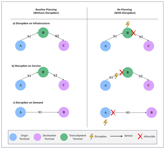
Figure 2.
Examples of potential impacts of a disruption on the network: (a) Impact on Infrastructure: The disruption affects the transshipment terminal (Port B), leading to extended transshipment times, which prevents the transshipment from being completed before the departure of service S2. (b) Impact on Service: The disruption delays the arrival of service S1 at the transshipment terminal, thereby hindering the transshipment process before service S2 departs. (c) Impact on Demand: The disruption impacts the origin port, resulting in an extended demand release time. Consequently, the demand cannot be released in time to connect with the departure of service S1.
4. Methodology
The methodology proposed in this research is structured and designed to advance the frameworks by [8,10,11,13] under the three primary modules: the offline planning module, the disruption module, and the re-planning module. An overview of the proposed methodology is depicted in Figure 3. Initially, the offline planning module formulates transportation plans, based on the previous work of the authors [8,13], without accounting for potential disruptions. This phase develops a baseline plan based on the order information, infrastructure details, and service data, using the AIT freight-optimization model.

Figure 3.
Proposed methodology [10,40].
Subsequently, the disruption module, an extension to the current disruption module developed in [10,11], operates as a continuous monitoring system that detects disruptions across the network, including those affecting network links (e.g., rail or road segments) or critical nodes (e.g., ports and terminals). Upon identifying a disruption, this module updates key variables impacted by the event, such as service times, loading and unloading duration, transshipment times, storage capacity, and release times for shipment requests. The disruption module is thus responsible for identifying disruptions and assessing their effects on the network environment.
Finally, the re-planning module determines appropriate responses to identified disruptions by utilizing one of the contributed strategies of this study “Reassign with Delay Buffer” or “(De)Consolidate” the shipment requests or the benchmark strategy of “Always Wait”. Each of these strategies provides a different approach to handling disruptions, ranging from waiting until the network is cleared to adjusting schedules and consolidating or deconsolidating shipments to maximize resource utilization and minimize delays. In the sections that follow, each of these modules and their respective components are detailed.
4.1. Baseline (Offline) Planning
A summary of the developed deterministic formulation of the AIT freight transportation model in [8,13] is presented in this section to facilitate a better understanding of its integration for matching decisions in the proposed framework. Subsequently, the associated heuristic algorithm for feasible path generation is also briefly presented as it will be used to enhance computational efficiency and reduce solution time in both offline and online planning modules.
4.1.1. Deterministic AIT Model Formulation
As mentioned in Section 3, we consider a global shipment matching platform under the AIT concept. According to the described problem (Figure 1), the deterministic mathematical formulation of the problem is presented as follows (See Table 2 for notations).
Table 2.
Notation used throughout the paper.
Subject to:
The objective function (1) attempts to maximize the number of matches and minimize the total transportation cost which includes seven terms: the first term enforces the model to match shipment requests as many as possible. The second term determines the transportation cost, the third term denotes transshipment cost, the fourth term accounts for storage cost, the fifth term shows the delay penalty costs, the sixth term computes canal-crossing cost ( is euqal to one for the routes and services that containts one or more marine service(s) that passes through a canal), the seventh term represents the loading/unloading cost, and the final term is the monetary value of emission based on service emissions and carbon tax.
Constraints (2) and (3) guarantee the platform accepts requests only if there are available services departing from the request’s origin and arriving at the request’s destination, respectively. Constraints (4) and (5) check that at most one service matches with request with the same origin and destination, respectively. Constraints (6) to (9) are responsible for eliminating subtours from the solution in which constraints (7) and (8) are designed to remove the subtours from shipment request origin and destination, respectively. Moreover, constraints (9) and (10) are designed so that each itinerary must have one origin and destination. Constraint (10) ensures flow conservation at transshipment terminals. Constraint (11) ensures that the total amount of containers matched with service does not surpass the service available capacity at the decision epoch . Constraint (12) guarantees that the departure time of service minus loading time (based on container volumes) should be earlier than the request release time, for matched requests and services. B is a large number to make the constraint valid when a request is matched with a service (i.e., ). Constraints (13)–(15) maintain the logic of the transshipment problem through binary variables and . The first one denotes the potential service that could be matched with service at where the destination of the transshipment service is similar to the request destination (i.e., ). The binary variable equals 1 if and only if and indicating that the transshipment occurred between service s and p. Constraint (16) ensures the temporal feasibility of transshipment at the intermediate terminal. Constraints (17) and (18) calculate the loading and unloading cost at the origin and destination of the request, respectively. Constraint (19) determines the transshipment cost including both loading and unloading costs at the transshipment terminal. Constraints (20)–(22) are designed to calculate storage cost. Constraint (20) determines the storage cost at the origin terminal. Constraint (21) computes the storage cost at the transshipment terminal, and constraint (22) determines the storage cost at the destination terminal. Constraint (23) determines the delay time at the destination intermodal terminal of the request. The final two constraints focus on managing the available infrastructure resources. Constraint (24) ensures that the total amount of storage used at any terminal does not exceed the terminal’s storage capacity. Constraint (25) ensures that the total transshipment operations at any transshipment terminal do not exceed the terminal’s transshipment capacity.
The formulation of our model draws inspiration from the methodologies presented in [8,15], but it introduces distinctions. The study by [15] assumes unlimited truck availability and models road travel time using a normal distribution, framing the problem within a stochastic programming context. This approach simplifies certain operational elements, as it omits infrastructure constraints such as terminal storage and transshipment capacity. Additionally, ref. [15] does not account for canal crossing cost in the objective function, an important factor in freight transportation networks where such transshipment points can incur substantial fees.
The study in [8] takes a different approach by treating road travel time as an uncertain factor modelled by a machine learning-based prediction model, formulating the problem through a robust optimization framework to mitigate the impact of variability in travel durations. Uncertain travel times can shift delivery windows and disrupt planned transshipments, thus affecting both route feasibility and service reliability. This deterministic approach allows for a clearer assessment of the disruption-handling strategies without the added complexity of uncertain travel times, enabling a more focused analysis of delay buffers and (De)Consolidation policies within a controlled environment.
Overall, while both previous studies offer valuable insights into synchromodal optimization under different assumptions, our model is uniquely positioned to explore the effects of deterministic travel times and operational constraints on disruption-management policies, providing a more grounded understanding of how these factors interact in a structured transportation network. This mathematical model applies optimization, specifically tailored for an AIT shipment matching problem. The objective function has been enhanced with a “canal crossing” cost component, reflecting the specific requirements of our case study. Furthermore, the formulation includes constraints related to infrastructure resource limitations, specifically terminal storage capacity and terminal transshipment capacity (Constraints (24) and (25)), ensuring the model’s applicability to real-world scenarios where such limitations are critical.
4.1.2. Feasible Path Generation Preprocessing-Based Heuristic Algorithm
Constraints (12)–(16) and (20)–(22) serve to verify the creation of paths (combinations of services), ensure the temporal feasibility of these paths, and compute the transshipment and storage costs at the transshipment terminals. These constraints considerably expand the solution search space, thus increasing the model’s computational complexity. To mitigate this complexity, a preprocessing algorithm is designed to evaluate the feasibility of path creation.
The preprocessing algorithm for feasible paths is described as follows: A path p is defined as a sequence of services. A path p is deemed viable if the services within the path meet time-spatial compatibility requirements. For two consecutive services and within path p, the destination of service must coincide with the origin of service (i.e., ). Additionally, the arrival time of service plus the unloading time at must be earlier than the departure time of service minus the loading time at the transshipment terminal. The term refers to the maximum number of services in a path. Let P denote the set of feasible paths, and represent the set of feasible paths with l services departing from terminal i and arriving at terminal j.
The pseudocode for preprocessing feasible paths is illustrated in Algorithm 1. The algorithm begins by identifying the feasible paths for each origin-destination pair with just one service, and then iteratively combines these paths with additional single services to generate feasible paths with two services, three services, and so forth, until the number of services reaches . To verify whether a new path , consisting of a feasible path and a service , is feasible, the algorithm checks the transshipment feasibility between services and using constraints (16) and (17), assuming , , which implies (satisfying constraints (13)–(15)). Subsequently, the algorithm checks for the presence of sub-tours within the feasible path and eliminates paths containing sub-tours. Finally, the transshipment cost is calculated using constraint (19).
| Algorithm 1 Feasible path generation algorithm |
Input: Intermodal Terminals I, Services S, , index , Storage Cost, Transshipment Cost Output: Feasible paths where , . Initialize: Let , . Checking Spatial Feasibility:
|
4.2. Disruption Module
The disruption module, which is an extension to the current disruption module developed in [10,11], plays a pivotal role in the real-time monitoring and adaptive management of disruptions within the transportation network. Upon detecting a disruption, the module evaluates its impact by referencing detailed disruption profiles outlined in Table 1. This evaluation process involves identifying the specific services and network nodes affected, based on the disruption’s characteristics, including modality, impact scope, and duration. When a disruption impacts a transportation service, the module updates both the departure and arrival times for the affected service, adjusting for delays and ensuring that these adjustments are consistent with the disruption’s timeline. Conversely, if the disruption affects a network node, such as a port or terminal, the module updates the node’s operational parameters. Specifically, it modifies loading/unloading times and transshipment durations to align with the disruption’s severity and duration. This ensures that all operational adjustments accurately reflect the disruption’s impact on the network.
One of the key distinctions of the disruption module in this study, compared to that of the previous work [10,11] is that the disruption modulel triggers the feasible path generation algorithm to ensure that routing decisions remain accurate and account for all relevant constraints. The feasible path generation algorithm was designed to construct paths by combining available services and verifying capacity and temporal feasibility for transshipment. Whenever there are updates to service schedules or node parameters, this algorithm dynamically reassesses path feasibility, by recalculating paths based on the latest service and infrastructure information. This process of re-evaluation and adaptation supports the AIT system’s ability to respond dynamically to disruptions, thereby enhancing the network’s resilience and robustness in maintaining service continuity. The psudocode of the disruption module is presented in Algorithm 2.
The disruption impact-assessment algorithm systematically categorizes disruptions based on whether they affect services or nodes. For service disruptions, it checks the relationship between the disruption period and the service’s departure and arrival times. If the service departs within the disruption period but arrives afterward, the algorithm adjusts the departure time to the disruption’s end and recalculates the arrival accordingly. If the service arrives within the disruption period but departs earlier, only the arrival time is adjusted. In cases where both departure and arrival fall within the disruption duration, the algorithm sets the departure to the disruption’s end and recalculates the arrival based on the revised schedule. For node disruptions, the algorithm increases loading/unloading and transshipment times for the affected node by the duration of the disruption. Additionally, it identifies shipment requests originating from the disrupted node and adjusts their release times to align with the end of the disruption, thereby ensuring that shipments are only released once normal operations have resumed.
To further assess the impact of disruptions, the module evaluates the entire transportation network under adjusted conditions, providing a comprehensive view of how delays and operational adjustments propagate throughout the system. This evaluation involves re-examining the viability of transport paths by re-running the path generation process specifically for paths that include disrupted services and matched shipment requests impacted by delays. In the “Always Wait” strategy, the path generation algorithm checks the feasibility of each path for updated shipment requests and delayed services. This involves adjusting path attributes based on newly available information, such as altered service schedules and extended delivery times, ensuring that paths remain feasible given the current network conditions. For the “Reassign with Delay Buffer” strategy, the path generation algorithm takes a more proactive approach by first filtering out services experiencing delays that exceed the defined delay buffer threshold. By excluding excessively delayed services, the algorithm ensures that only reliable and timely services are considered in the re-planning process. Once these adjustments are made, the algorithm proceeds to generate feasible paths that prioritize resilience and efficiency. This selective path generation approach not only reduces the risk of further delays but also optimizes resource utilization by preventing the assignment of disrupted services to time-sensitive shipments. This approach enables decision-makers to visualize potential bottlenecks and identify areas where resilience strategies are most needed. The insights gained from this analysis not only facilitate immediate responses to the current disruption but also help to inform longer-term strategies for improving the network’s overall resilience to future disruptions.
| Algorithm 2 Disruption module algorithm |
Input: Set of Services S, Set of Shipment Requests R, Set of Disruptions Output: Updated Services S, Updated Shipment Requests R, Feasible Paths
|
4.3. Re-Planning (Online Planning) for Disruption
The re-planning, or online planning, module serves as the core component of the methodology, by employing two new strategies of “Reassign with Delay Buffer”, and “(De)Consolidation”. The overall conceptual framework of the re-planning module is built upon the work in [10,11] and advancing them by introducing and evaluating the new strategies of “Reassign with Delay Buffer”, and “(De)Consolidation” in addition to the benchmark strategy of “Always Wait”. Each strategy offers a unique approach to mitigating the effects of disruptions, catering to different operational needs and resilience strategies. The following sections provide a detailed explanation of each strategy, highlighting their respective mechanisms and decision-making processes for handling disruptions in the freight transportation network.
4.3.1. Reassign with Delay Buffer
The “Reassign with Delay Buffer” strategy provides a balanced approach to handling disruptions by allowing affected services to be delayed up to a specified threshold before rerouting is considered [Algorithm 3]. This strategy starts by assessing each service’s route against any active disruptions. If a disruption affects a service, the delay incurred by the disruption is calculated, and the service’s departure and arrival times are adjusted accordingly. The delay is then compared to a predefined threshold, representing the maximum allowable delay. If the delay falls within this buffer, the service is retained as available, ensuring continuity with a minor tolerance for delay. However, if the delay exceeds the threshold, the service is marked as unavailable, signaling that rerouting is necessary to avoid unacceptable delays.
Following the delay evaluation, the algorithm filters out unavailable services and reconstructs feasible paths using only the remaining available services. By generating paths based on this updated set, the platform effectively adapts to disruption impacts while maintaining service reliability within the constraints of the delay buffer. Shipment requests are then matched to feasible paths through an optimization model that aims to minimize costs or maximize efficiency, considering updated service capacities and timelines. This approach enhances the resilience of the transportation network, allowing for a measured tolerance of delays without sacrificing overall service performance. By incorporating a delay buffer, the strategy provides flexibility in responding to disruptions while ensuring that the service network remains robust and capable of meeting delivery requirements.
To evaluate the flexibility of the Reassign with Delay Buffer strategy, we tested three delay-tolerance thresholds: 2, 4, and 6 h. These values represent varying levels of operational conservatism, with lower thresholds triggering faster reassignment and higher thresholds allowing more delay absorption. The selected range reflects typical time intervals observed in intermodal freight operations and enables a structured sensitivity analysis of the strategy’s responsiveness. These threshold values are not intended to be prescriptive and should be adapted based on the specific characteristics and requirements of the application setting.
| Algorithm 3 Reassign with delay buffer strategy |
Input: Updated Set of Impacted Shipment Requests , Updated Set of Impacted Services , Set of Disruptions , Delay Threshold , Planning Horizon T Output: Acceptance decision , Matching decision , Objective function (minimized cost)
|
4.3.2. (De)Consolidation
This disruption-handling strategy centers on two primary strategies: consolidation and deconsolidation. In the case of consolidation, the model attempts to combine multiple shipment requests onto a single or limited number of services. This approach is particularly effective when there are constraints on service availability, allowing the model to optimize resource utilization by grouping shipments. Consolidation can streamline operations, reduce overall transportation costs, and alleviate service shortages by maximizing the use of available capacity on fewer services. Conversely, the deconsolidation strategy involves splitting a single shipment request across multiple services. This option becomes essential when no individual service has sufficient capacity to accommodate the entire shipment request. The model addresses service capacity limitations by splitting large shipments across multiple services. This approach ensures timely delivery even when no single service can accommodate the entire request. Deconsolidation thus enables greater flexibility in service selection, allowing the model to leverage the cumulative capacity of multiple services rather than depending on a single service.
Together, these strategies provide a robust framework for managing disruptions within a freight network. Consolidation addresses scenarios where service availability is restricted, while deconsolidation facilitates efficient shipment handling when the network offers multiple services, none of which independently meet the shipment’s capacity needs. This dual approach enhances the model’s ability to adapt to changing operational conditions and makes the transportation system more resilient to disruptions. To operationalize this strategy, an optimization model has been formulated to derive the necessary decisions for handling disruptions. This model systematically evaluates consolidation and deconsolidation options by analyzing service capacity, shipment requirements, and network conditions. By incorporating constraints and objective functions tailored to the specific needs of consolidation and deconsolidation, the model ensures that each decision aligns with overall operational goals.
The objective function presented in Equation (26) builds upon the deterministic objective function outlined in Equation (1), sharing the first eight terms. These initial terms encompass the primary costs associated with the AIT shipment matching process, including the penalties for unmatched requests, transportation costs across services, transshipment costs, storage costs, delay penalties, canal-crossing costs, loading/unloading costs, and emission costs. In addition to these fundamental terms, two additional components are introduced to explicitly account for the operational costs of consolidation and deconsolidation. These latter terms model the handling costs incurred when shipments are consolidated or deconsolidated at terminals, capturing the expenses tied to the time and labor required for these processes. The consolidation cost term represents the additional costs for combining smaller shipments into larger ones at specific points in the network, while the deconsolidation cost term reflects the disaggregation of shipments upon reaching transshipment or final destinations.
Subject to:
Constraint (27) enforces that each shipment must select exactly one of three possible actions: consolidation, deconsolidation, or no change. This exclusivity ensures that each shipment follows a single operational pathway, which is critical for maintaining both clarity and feasibility within the AIT network. By limiting each shipment to one action, the model avoids conflicting assignments and simplifies decision-making processes. Constraint (28) upholds the capacity limitations of each service by ensuring that the cumulative volume of all shipments assigned to a given service does not exceed its maximum capacity. This constraint is essential for respecting the physical limitations of transportation assets and prevents overloading, which would otherwise compromise operational efficiency and service reliability. Calculating the storage and delay times for different scenarios—namely, no change, consolidation, and deconsolidation—involves the multiplication of decision variables, such as . This multiplication leads to nonlinearity in the model, rendering it unsuitable for standard optimization solvers. To address this, constraints (29) through (37), along with (42) through (50), are designed to linearize the product of binary variables. This linearization technique facilitates the application of linear programming solvers, enhancing the model’s computational tractability.
Additionally, constraints (38) through (41) are specifically structured to compute the storage time for each shipment under the different operational scenarios. By accurately calculating the storage time, these constraints contribute to a more precise estimation of storage costs in the objective function. Constraint (51) calculates the delay time for shipments that do not meet their scheduled delivery times, which is subsequently used to impose delay penalties within the objective function. To limit the operational complexity of deconsolidation, constraint (52) restricts the maximum number of services that a shipment can use for deconsolidation. This ensures that the system remains manageable and that deconsolidation activities do not exceed predefined operational thresholds. Finally, constraints (53) and (54) enforce the temporal feasibility of consolidation and deconsolidation activities, respectively, ensuring that these operations can be executed within the available time windows.
4.3.3. Always Wait
The “Always Wait” strategy is a conservative and intuitive strategy used to handle disruptions by waiting for affected shipment requests, ports, and services to resume rather than seeking alternative routes [7,10]. This approach is based on the premise that shipments should maintain their originally planned connections even if delays occur, thereby preserving continuity within the transportation network. Under this strategy, whenever a disruption impacts a terminal, the affected services simply wait until the terminal operations return to normal. This ensures that the transshipment connections are maintained, although the shipment may experience delays. Such a strategy is particularly suitable when the emphasis is on maintaining established service routes, or when re-routing would be costly or logistically impractical. However, this strategy might lead to infeasible plans, for instance, consider a disrupted port, and the re-planning under the Always Wait strategy updates the shipment request release time to the end of the disruption. The service that is previously matched with this service is gone and the shipment request is released after the service departure. The pseudocode for the “Always Wait” strategy is presented in Algorithm 4.
| Algorithm 4 Always Wait strategy disruption-handling algorithm |
Input: Updated Set of Impacted Shipment Requests , Updated Set of Impacted Services , Set of Disruptions , Planning Horizon T Output: Acceptance decision , Matching decision , Objective function (minimized cost)
|
5. Numerical Experiments
In this section, we present extensive numerical experiments conducted to evaluate the performance and effectiveness of the proposed framework. The entire modeling framework, including the optimization model, was implemented in Python, with the commercial GUROBI solver employed to handle the mixed-integer linear programming (MILP) formulations. The experiments were executed on a computational setup consisting of an 11th Gen Intel(R) Core(TM) i7-11850H processor, running at 2.50 GHz, supported by 32GB of RAM.
5.1. Experimental Setup
The AIT model logistic and network parameters are set as follows: planning horizon (unit: hours) (Two weeks); decision epoch time interval ; loading time (unit: minutes/TEU) ,, , for ; loading cost (unit: USD/TEU) , , , for ; storage cost (unit: USD/TEU-h) for ; delay cost (unit: USD/request-h) for ; carbon tax (unit: USD/kg) ; and canal crossing cost (unit: USD/TEU) . Without loss of generality in the framework, and were considered sufficiently large to always satisfy infrastructure-related constraints (Constraints (24) and (25)).
The case study focuses on the Great Lakes region, where the Welland Canal plays a critical role in connecting Lake Ontario to Lake Erie. This strategic waterway enables marine services to bypass Niagara Falls, facilitating continuous freight movement between inland ports and supporting multimodal transport integration across the region. The proposed model was tested on an intermodal terminal network within the Great Lake region, as depicted in Figure 4. To construct the demand side of the model, data was extracted from the “STATSCAN transborder trade database,” which contains over 30 million records at the commodity level, specifically detailing trade movements within the Great Lake area [46]. For this study, a sample dataset of 300 shipment requests, amounting to a total of 2500 TEU over two weeks, was selected. This sample aligns proportionally with port throughput data from 2016 to 2020, ensuring that it reflects realistic trade flows within the region. According to the “Transport Canada Annual Report 2022,” approximately 17% of the total port throughput in Canada consists of containerized cargo, as outlined in the Transportation in Canada 2022 report. While this percentage may not precisely apply to the Great Lake region, it serves as a valuable reference point. Based on this, we assumed that 20% of the regional port throughput is comprised of containerized cargo, a proportion that reflects both the Transport Canada report and recent investments by the Canadian government in container infrastructure at these ports. This assumption guided the generation of the demand dataset, providing a realistic representation of containerized cargo flows for this analysis.

Figure 4.
Geographical scope of the case study (base map is adopted from Google Earth).
The service dataset was constructed using synthetic data specifically tailored for the Great Lakes region. This dataset encompasses a diverse range of transportation services, including two train services, one marine service, and two fleets of trucks for each origin-destination pair within the intermodal terminal network. Each truck fleet consists of 20 trucks, providing flexibility and capacity to meet various demand requirements. By incorporating multiple transportation modes—marine, rail, and truck—this dataset effectively represents the logistics capabilities of the Great Lakes intermodal transportation network. This synthetic dataset was designed to reflect realistic service options and capacities, capturing the unique operational dynamics within the region. By ensuring the availability of different modes of transportation, the dataset supports robust operational planning and enables comprehensive analysis of adaptive transport strategies. As a result, it provides a valuable foundation for evaluating the effectiveness of the proposed optimization model in handling complex, multimodal service networks.
In addition, based on the disruption profiles detailed in Table 1, randomly generated disruption scenarios were sampled to evaluate the robustness of the proposed model. These scenarios represent a wide range of disruption events, with varying levels of intensity and impact. The number of disruptions generated in each scenario differs, enabling a comprehensive assessment of how the model performs under different stress conditions. The disruption scenarios utilized in the numerical experiments are strategically designed to challenge the model’s capabilities in handling disruptions across various layers of the transportation network, such as services, nodes, and links. These scenarios provide insights into the model’s ability to optimize performance when faced with operational uncertainties, ensuring that the system remains resilient even in the presence of severe or unexpected disruptions. The full details of these scenarios are presented in Table 3.
Table 3.
Disruption scenarios and their impact.
5.2. Results and Discussion
Extensive numerical experiments were conducted to assess the performance of different disruption-handling strategies across three disruption scenarios: low, medium, and high disruptions. Figure 7 illustrates the cost per container under various strategies, allowing us to compare their effectiveness while normalizing the results by shipment size to remove the impact of matching percentages.
We examined three main strategies in these experiments:
- Always Wait Strategy: A reactive strategy where shipments are delayed until the service resumes.
- Reassign with Delay Buffer Strategy: A proactive strategy that reassigns shipments to available services, with three delay buffer thresholds: 2, 4, and 6 h.
- (De)Consolidation Strategy: A novel strategy designed to dynamically consolidate or deconsolidate shipments, based on service availability and capacity.
The low-disruption scenario results (Figure 5a) indicate that the Always Wait Strategy performs the worst, resulting in significantly higher costs per container. The Reassign with Delay Buffer strategy demonstrates a substantial improvement in performance, with very similar outcomes observed for the 4 h and 6 h delay buffers. In this scenario, the (De)Consolidation strategy emerges as the most effective, delivering the lowest cost per container, owing to the flexibility of consolidating shipments when needed. In the medium-disruption scenario (Figure 5b), the Reassign with Delay Buffer strategy shows a performance that is closer to the Always Wait strategy. This is likely due to the increased number of disrupted services compared to the low-disruption scenario, limiting the effectiveness of reassigning shipments. The 6 h delay buffer slightly outperforms the other delay thresholds, but the difference is marginal. The (De)Consolidation strategy continues to outperform the other strategies, though the margin of improvement is smaller than in the low-disruption scenario.
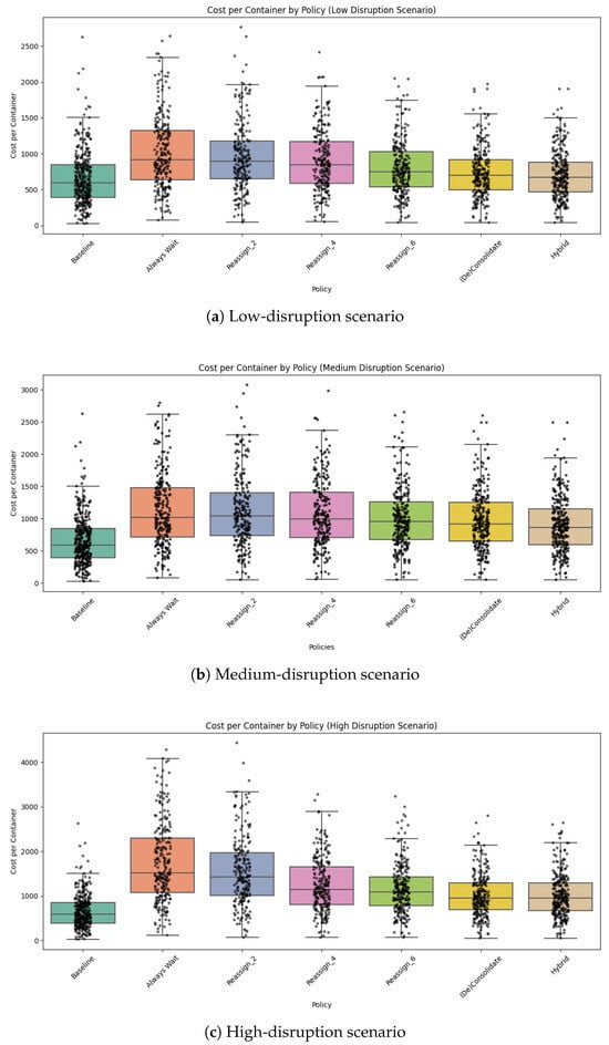
Figure 5.
Cost per container under different disruption scenarios: (a) low disruption, (b) medium disruption, and (c) high disruption.
For the high-disruption scenario (Figure 5c), the results demonstrate a significant increase in costs for the Always Wait strategy, as the number of disrupted services and nodes is much higher. The Reassign with Delay Buffer strategy shows substantial improvement over the Always Wait strategy, with the impact of the delay buffer becoming more pronounced. The 6 h buffer results in notably lower costs compared to the 2 h and 4 h buffers. In this severe disruption context, the (De)Consolidation strategy shows its greatest advantage, providing the most cost-effective solution. The performance gap between the (De)Consolidation strategy and the Reassign strategy becomes more visible in this scenario, highlighting the robustness of the (De)Consolidation strategy in high-disruption environments. Overall, the experimental results suggest that in low-disruption scenarios, reassigning shipments and consolidating them results in significant cost savings. However, as the disruption severity increases, the (De)Consolidation strategy consistently provides superior results, especially when service availability becomes highly constrained.
The analysis of disruption-handling strategies based on Table 4 shows that in the low-disruption scenario, the (De)Consolidation strategy outperforms other strategies in terms of both cost and effectiveness. It achieves the highest matched percentage at 83% and the lowest total cost per TEU at 694 while incurring only 3% in disruption costs. The Always Wait strategy, on the other hand, performs poorly with a lower matched percentage (69%) and higher disruption costs per TEU (23%). The Reassign strategies show gradual improvement as the delay threshold increases, with the 6 h delay buffer providing a significant reduction in total cost per TEU (718) and a lower percentage of lost shipments (10%) compared to the 2 h and 4 h thresholds. This indicates that the flexibility offered by higher delay thresholds allows for better operational adjustments and cost efficiency in handling disruptions.
Table 4.
Strategy comparison with costs and disruption effects.
In the medium- and high-disruption scenarios, the performance gap between strategies becomes more pronounced. In both cases, the (De)Consolidation strategy remains the most effective in minimizing disruption costs and lost shipments, with the lowest cost per TEU and lost shipment percentage. However, in the high-disruption scenario, the Always Wait strategy results in a significant increase in costs, with a total cost per TEU of 1459 and a high disruption-incurred cost per TEU of 116%, indicating that it is not suitable for more severe disruptions. The Reassign strategies, especially with the 6 h delay threshold, show improved performance, reducing total costs and disruption effects. This highlights the advantage of more flexible, dynamic strategies like Reassign and (De)Consolidation in handling larger-scale disruptions effectively, ensuring lower operational costs and better shipment matching.
Figure 6 compares the disruption-incurred cost per TEU across different strategies under three disruption scenarios: low, medium, and high. Among all the strategies, the (De)Consolidation strategy consistently shows the lowest disruption-incurred costs across all scenarios, particularly excelling in the high-disruption scenario where the cost is significantly lower than other strategies. The “Always Wait” strategy, on the other hand, incurs the highest costs, with the disruption-incurred cost surpassing 100% in the high-disruption scenario. Reassigning strategies with varying delay thresholds (2, 4, and 6 h) perform progressively better as the delay threshold increases, although none perform as well as the (De)Consolidation strategy. The reassign with a 6 h delay performs better than the 2 h and 4 h delays but still incurs higher costs than the (De)Consolidation approach. This comparison highlights the effectiveness of (De)Consolidation in mitigating the costs associated with disruptions and demonstrates its superiority over other adaptive strategies in reducing disruption-related expenses.
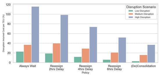
Figure 6.
Disruption-incurred cost per TEU by strategy and disruption scenario compared to the baseline scenario (without disruption).
The series of six figures presented in Figure 7 offers a comparative analysis of storage hours and delay hours across low, medium, and high-disruption scenarios for various strategies. In the low-disruption scenario, depicted in Figure 7a,b, the “Always Wait” strategy leads to the highest storage and delay hours, as well as a significant drop in match percentage. The reassign strategies with varying delay thresholds show gradual improvements in both storage and delay hours, alongside an increase in match percentage. The (De)Consolidation strategy performs the best in this scenario, minimizing storage and delay hours while maintaining a high match percentage. The medium-disruption scenario, represented by Figure 7c,d, demonstrates a more pronounced impact of disruption. Storage and delay hours increase across all strategies compared to the low-disruption scenario. Similar to the previous scenario, the “Always Wait” strategy performs the worst, while the reassign strategies progressively improve performance as the delay threshold increases. The (De)Consolidation strategy remains the best-performing option, achieving the least storage and delay hours, and the highest match percentage. Finally, the high-disruption scenario, shown in Figure 7e,f, highlights the severe impact of disruptions. The “Always Wait” strategy results in the highest delay hours and the lowest match percentage. The reassign strategies again show improvements in performance as the delay threshold increases, but the overall effect of disruption is much more significant in this scenario. Even though the (De)Consolidation strategy still performs the best in terms of minimizing delays and maximizing match percentage, its performance also declines in comparison to the less severe disruption scenarios.
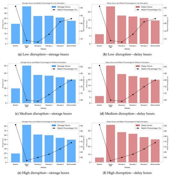
Figure 7.
Comparison of storage hours and delay hours across disruption severity levels: (a,b) low disruption, (c,d) medium disruption, and (e,f) high disruption.
To clarify the impact of (De)Consolidation costs on the disruption module’s outcomes, we conducted a sensitivity analysis on consolidation and deconsolidation cost ( and ) parameters. Figure 8 visualizes how the use of the (De)Consolidation strategy varies with increasing unit consolidation costs under three disruption scenarios. As expected, higher consolidation costs lead to a consistent decline in the adoption of this strategy across all scenarios. In the high-disruption setting, reliance on (De)Consolidation remains relatively strong even at higher cost levels, highlighting its importance for maintaining flow continuity during network stress. Conversely, in the low-disruption scenario, operators appear more cost-averse and quickly reduce the use of this strategy as costs increase, indicating greater flexibility when the network is otherwise functioning well. This analysis underscores the importance of tailoring disruption-response strategies to network conditions. In highly disrupted environments, policy should support investment in scalable consolidation infrastructure and perhaps offer subsidies or incentives to offset higher consolidation costs. For operators, this also means preparing cost-contingent contingency plans that factor in how cost tolerance affects strategic decisions. Furthermore, public agencies might consider dynamic pricing models or risk-sharing mechanisms to encourage more consistent usage of (De)Consolidation under stress, ensuring more resilient supply chain operations across varying disruption levels.
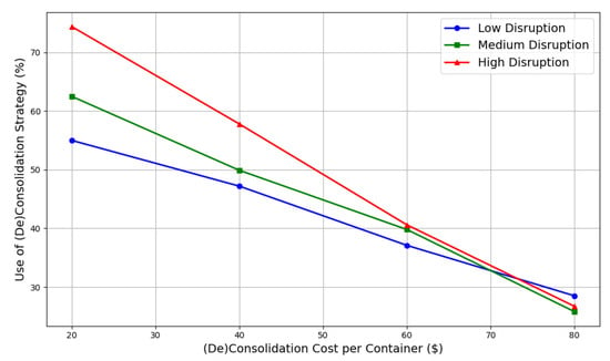
Figure 8.
Use of the (De)Consolidation strategy decreases as unit consolidation cost rises. The decline is sharper under low disruption, while high-disruption scenarios maintain higher usage, reflecting greater operational necessity.
6. Conclusions
Disruptions are an inherent aspect of transportation networks, often rendering parts of pre-planned deliveries infeasible due to network constraints and unexpected events. This study highlights the need to integrate effective disruption-management strategies into freight transport processes. Our evaluation of the proposed strategies—Reassign with Delay Buffers and (De)Consolidation—shows that these adaptive methods enhance network resilience and responsiveness. Even under mild disruptions, some deliveries may fail, reinforcing the need for disruption-aware models to ensure flexibility and operational continuity.
As disruptions increase, the value of consolidation strategies becomes more evident. The (De)Consolidation strategy consistently outperformed others in medium- to high-disruption scenarios by optimizing capacity use and reducing costs. However, its practical implementation may face logistical challenges and capacity limitations at service nodes. Moreover, consolidation costs can influence assignment decisions and overall effectiveness, emphasizing the need for careful cost-benefit evaluation when choosing a disruption-handling approach.
The problem studied in this paper offers several avenues for future research. First, as the scale of transportation networks in real-world applications increases, there is a growing need for more computationally efficient solutions. Developing heuristic or metaheuristic methods that provide timely and high-quality solutions can help tackle the complexity of large-scale transportation networks, allowing for faster decision-making under dynamic conditions. Second, incorporating cargo prioritization into the model can enhance its practical applicability. By prioritizing cargo based on its value, urgency, or customer requirements, the model can allocate resources more efficiently, ensuring that high-priority shipments are handled with greater speed and care, particularly during disruption scenarios.
Third, while the current model adopts a reactive disruption-management approach—where re-planning is triggered only when a disruption is detected—there is potential to explore proactive disruption-management strategies. Proactive methods aim to anticipate potential disruptions using predictive analytics or simulation models, enabling the system to prepare mitigation strategies in advance. This would improve the model’s responsiveness and robustness in dealing with uncertainties. However, implementing such approaches requires advanced disruption forecasting techniques, which could be developed using historical data, real-time monitoring, or simulation-based models. Fourth, although this study adopts a mid-sized experimental setup for clarity and computational efficiency, the underlying framework is designed to scale to larger, more complex networks. Future research will focus on validating the model under higher shipment volumes and longer planning horizons to evaluate the broader applicability and resilience of the proposed strategies. Fifth, given the multiple strategies available for handling disruptions, a promising direction for future research is the integration of reinforcement learning. By training an agent to select the optimal strategy based on the current state of the network, service availability, demand conditions, and ongoing disruptions, the model could autonomously adapt to varying scenarios, improving its decision-making capabilities over time. This would offer a more dynamic and intelligent approach to disruption management, enhancing the flexibility and resilience of the AIT transportation system.
As a final direction for future research and implementation, the integration of emerging digital technologies such as the Internet of Things (IoT) and blockchain presents a promising opportunity to enhance the operationalization of the proposed disruption-handling strategies [47]. While the current study focuses on the optimization and evaluation of strategies like Reassign with Delay Buffer and (De)Consolidation, these mechanisms can be further strengthened by embedding them within digitally enabled logistics systems. IoT technologies provide real-time data on shipment locations, terminal processes, service disruptions, and transit delays—enabling the dynamic activation of reassignment or consolidation decisions as disruptions unfold. This increased visibility could improve both responsiveness and reliability in time-sensitive freight operations. Blockchain, on the other hand, offers a secure and decentralized ledger that can record and trace strategy activations, rerouting decisions, and transshipment actions in a tamper-proof manner. This is particularly valuable in multi-stakeholder environments where transparency, trust, and verifiability are critical. Exploring the interoperability of these technologies with adaptive intermodal frameworks could enable more resilient, automated, and auditable disruption-management systems in future freight networks.
Author Contributions
Conceptualization, S.F., M.S. and S.R.; methodology, S.F., M.S. and S.R.; software, S.F. and S.D.; validation, S.F., M.S. and S.R.; formal analysis, S.F.; investigation, S.F. and S.D.; resources, M.S. and S.R.; data curation, S.D.; writing—original draft preparation, S.F.; writing—review and editing, S.F., M.S. and S.R.; visualization, S.F.; supervision, M.S. and S.R.; project administration, M.S. and S.R. All authors have read and agreed to the published version of the manuscript.
Funding
This research was partially funded by LIVERPOOL-MCMASTER GPF BBSRC FUND.
Data Availability Statement
The datasets presented in this article are not readily available because of privacy and legal rights.
Conflicts of Interest
The authors declare that they have no known competing financial interests or personal relationships that could have appeared to influence the work reported in this paper. During the preparation of this work the authors used Chat GPT in order to fine-tune the article writing style. After using this tool/service, the authors reviewed and edited the content as needed and take full responsibility for the content of the publication.
References
- Li, R.; Li, L.; Wang, Q. The impact of energy efficiency on carbon emissions: Evidence from the transportation sector in Chinese 30 provinces. Sustain. Cities Soc. 2022, 82, 103880. [Google Scholar] [CrossRef]
- Demir, E.; Huang, Y.; Scholts, S.; Woensel, T.V. A selected review on the negative externalities of the freight transportation: Modeling and pricing. Transp. Res. Part E Logist. Transp. Rev. 2015, 77, 95–114. [Google Scholar] [CrossRef]
- McKinnon, A. Freight transport in a low-carbon world: Assessing opportunities for cutting emissions. TR News 2016. [Google Scholar] [CrossRef]
- Sakti, S.; Zhang, L.; Thompson, R.G. Synchronization in synchromodality. Transp. Res. Part E Logist. Transp. Rev. 2023, 179, 103321. [Google Scholar] [CrossRef]
- Tavasszy, L.; Behdani, B.; Konings, R. Intermodality and Synchromodality. In Ports and Networks; Routledge: London, UK, 2017; pp. 251–266. [Google Scholar] [CrossRef]
- Zanjirani Farahani, N.; Noble, J.S.; McGarvey, R.G.; Enayati, M. An advanced intermodal service network model for a practical transition to synchromodal transport in the US Freight System: A case study. Multimodal Transp. 2023, 2, 100051. [Google Scholar] [CrossRef]
- Hrušovskỳ, M.; Demir, E.; Jammernegg, W.; Van Woensel, T. Real-time disruption management approach for intermodal freight transportation. J. Clean. Prod. 2021, 280, 124826. [Google Scholar] [CrossRef]
- Filom, S.; Razavi, S. A learning-based robust optimization framework for synchromodal freight transportation under uncertainty. Transp. Res. Part E Logist. Transp. Rev. 2025, 195, 103967. [Google Scholar] [CrossRef]
- Frémont, A.; Franc, P. Hinterland transportation in Europe: Combined transport versus road transport. J. Transp. Geogr. 2010, 18, 548–556. [Google Scholar] [CrossRef]
- Dewantara, S. Resilient Synchromodal Transport Through Learning Assisted Hybrid Simulation Optimization Model. 2024. Available online: https://resolver.tudelft.nl/uuid:8ebaa55b-8df6-4fde-8522-9d95b8f98493 (accessed on 29 October 2024).
- Dewantara, S.; Filom, S.; Razavi, S.; Atasoy, B.; Saeednia, M. Resilient Synchromodal Transport through Learning Assisted Hybrid Simulation Optimization Model. arXiv. to be submitted to the Transportation Research Part C: Emerging Technologies.
- Fazi, S.; Fransoo, J.C.; Woensel, T.V. A decision support system tool for the transportation by barge of import containers: A case study. Decis. Support Syst. 2015, 79, 33–45. [Google Scholar] [CrossRef]
- Filom, S.; Razavi, S. Decarbonization through Modal Shift using a Synchromodal Platform: A Case Study in the Great Lakes. J. Supply Chain Manag. Sci. 2023, 4, 97–113. [Google Scholar] [CrossRef]
- Ferjani, A.; El Yaagoubi, A.; Boukachour, J.; Duvallet, C. An optimization-simulation approach for synchromodal freight transportation. Multimodal Transp. 2024, 3, 100151. [Google Scholar] [CrossRef]
- Guo, W.; Atasoy, B.; Negenborn, R.R. Global synchromodal shipment matching problem with dynamic and stochastic travel times: A reinforcement learning approach. Ann. Oper. Res. 2022, 2022, Guo2022. [Google Scholar] [CrossRef]
- Guo, W.; Zhang, Y.; Li, W.; Negenborn, R.R.; Atasoy, B. Augmented Lagrangian relaxation-based coordinated approach for global synchromodal transport planning with multiple operators. Transp. Res. Part E Logist. Transp. Rev. 2024, 185, 103535. [Google Scholar] [CrossRef]
- Rivera, A.E.; Mes, M.R. Anticipatory scheduling of synchromodal transport using approximate dynamic programming. In Annals of Operations Research; Springer: Berlin/Heidelberg, Germany, 2022; pp. 1–35. [Google Scholar] [CrossRef]
- Karbasi, A.H.; Mehrabani, B.B.; Cools, M.; Sgambi, L.; Saffarzadeh, M. Comparison of speed-density models in the age of connected and automated vehicles. Transp. Res. Rec. 2023, 2677, 849–865. [Google Scholar] [CrossRef]
- Zhang, J.; Sun, Y.; Feng, Q.; Zhao, Y.; Wang, Z. Data-Driven Robust Optimization of the Vehicle Routing Problem with Uncertain Customers. Complexity 2022, 2022, 9064669. [Google Scholar] [CrossRef]
- Farahani, A.; Genga, L.; Dijkman, R. Online multimodal transportation planning using deep reinforcement learning. In Proceedings of the 2021 IEEE International Conference on Systems, Man, and Cybernetics (SMC), Melbourne, Australia, 17–20 October 2021; IEEE: Piscataway Township, NJ, USA, 2021; pp. 1691–1698. [Google Scholar]
- Ambra, T.; Macharis, C. Agent-based digital twins (ABM-DT) in synchromodal transport and logistics: The fusion of virtual and pysical spaces. In Proceedings of the 2020 Winter Simulation Conference (WSC), Orlando, FL, USA, 14–18 December 2020; IEEE: Piscataway Township, NJ, USA, 2020; pp. 159–169. [Google Scholar]
- Alaei, S.; Durán-Micco, J.; Macharis, C. Synchromodal transport re-planning: An agent-based simulation approach. Eur. Transp. Res. Rev. 2024, 16, 1. [Google Scholar] [CrossRef]
- Kurapati, S.; Kourounioti, I.; Lukosch, H.; Bekebrede, G.; Tavasszy, L.; Verbraeck, A.; Groen, D.; Van Meijeren, J.; Lebesque, L. The role of Situation Awareness in Synchromodal Corridor Management: A simulation gaming perspective. Transp. Res. Procedia 2017, 27, 197–204. [Google Scholar] [CrossRef]
- Karbasi, A.H.; Zheng, N.; O’Hern, S. Investigating the Impact of Automated Vehicles on the Safety and Operation of Low-Speed Urban Networks. J. Adv. Transp. 2024, 2024, 3835831. [Google Scholar] [CrossRef]
- Halakoo, M.; Yang, H.; Biswas, A.; Azer, P.; Wang, J. A model predictive emission controller based on the heterogeneity aware emission macroscopic fundamental diagram. J. Clean. Prod. 2025, 493, 144907. [Google Scholar] [CrossRef]
- Delbart, T.; Molenbruch, Y.; Braekers, K.; Caris, A. Uncertainty in Intermodal and Synchromodal Transport: Review and Future Research Directions. Sustainability 2021, 13, 3980. [Google Scholar] [CrossRef]
- Rentschler, J.; Elbert, R.; Weber, F. Promoting Sustainability through Synchromodal Transportation: A Systematic Literature Review and Future Fields of Research. Sustainability 2022, 14, 13269. [Google Scholar] [CrossRef]
- Van Riessen, B.; Negenborn, R.R.; Lodewijks, G.; Dekker, R. Impact and relevance of transit disturbances on planning in intermodal container networks using disturbance cost analysis. Marit. Econ. Logist. 2015, 17, 440–463. [Google Scholar] [CrossRef]
- Qu, W.; Rezaei, J.; Maknoon, Y.; Tavasszy, L. Hinterland freight transportation replanning model under the framework of synchromodality. Transp. Res. Part E Logist. Transp. Rev. 2019, 131, 308–328. [Google Scholar] [CrossRef]
- Gao, S.; Liu, N. Improving the resilience of Port–Hinterland container logistics transportation systems: A bi-level programming approach. Sustainability 2021, 14, 180. [Google Scholar] [CrossRef]
- Karam, A.; Reinau, K.H. A real-time decision support approach for managing disruptions in line-haul freight transport networks. IEEE Trans. Intell. Transp. Syst. 2022, 23, 24765–24777. [Google Scholar] [CrossRef]
- Durán-Micco, J.; Jordehi, S.A.; Macharis, C. Evaluating synchromodal transport with agent-based simulation. Transp. Res. Procedia 2023, 72, 619–626. [Google Scholar] [CrossRef]
- Darayi, M.; Barker, K.; Santos, J.R. Component importance measures for multi-industry vulnerability of a freight transportation network. Netw. Spat. Econ. 2017, 17, 1111–1136. [Google Scholar] [CrossRef]
- Nair, R.; Avetisyan, H.; Miller-Hooks, E. Resilience framework for ports and other intermodal components. Transp. Res. Rec. 2010, 2166, 54–65. [Google Scholar] [CrossRef]
- Stamos, I.; Mitsakis, E.; Salanova, J.M.; Aifadopoulou, G. Impact assessment of extreme weather events on transport networks: A data-driven approach. Transp. Res. Part D Transp. Environ. 2015, 34, 168–178. [Google Scholar] [CrossRef]
- Larsen, R.B.; Guo, W.; Atasoy, B. A real-time synchromodal framework with co-planning for routing of containers and vehicles. Transp. Res. Part C Emerg. Technol. 2023, 157, 104412. [Google Scholar] [CrossRef]
- He, Z.; Navneet, K.; van Dam, W.; Van Mieghem, P. Robustness assessment of multimodal freight transport networks. Reliab. Eng. Syst. Saf. 2021, 207, 107315. [Google Scholar] [CrossRef]
- Zhang, Y.; Negenborn, R.R.; Atasoy, B. Synchromodal freight transport re-planning under service time uncertainty: An online model-assisted reinforcement learning. Transp. Res. Part C Emerg. Technol. 2023, 156, 104355. [Google Scholar] [CrossRef]
- Filom, S.; Amiri, A.M.; Razavi, S. Applications of machine learning methods in port operations—A systematic literature review. Transp. Res. Part E Logist. Transp. Rev. 2022, 161, 102722. [Google Scholar] [CrossRef]
- Filom, S.; Razavi, S. Advancing Travel Time Prediction in Intelligent Transportation Systems Through Leaning-Based Uncertainty Quantification. In Proceedings of the 2024 IEEE International Conference on Smart Mobility (SM), Niagara Falls, ON, Canada, 16–18 September 2024; IEEE: Piscataway Township, NJ, USA, 2024; pp. 165–170. [Google Scholar]
- Di Febbraro, A.; Sacco, N.; Saeednia, M. An agent-based framework for cooperative planning of intermodal freight transport chains. Transp. Res. Part C Emerg. Technol. 2016, 64, 72–85. [Google Scholar] [CrossRef]
- Halakoo, M.; Yang, H.; Karbasi, A.H.; Farid, Y.Z.; Ucar, S.; Oguchi, K. Quantifying the Impact of Bottlenecks on Network Performance Using Macroscopic Fundamental Diagram Using Clustering and Decision Tree Prediction. Preprints 2023. [Google Scholar] [CrossRef]
- Akyüz, M.H.; Dekker, R.; Sharif Azadeh, S. Partial and complete replanning of an intermodal logistic system under disruptions. Transp. Res. Part E Logist. Transp. Rev. 2023, 169, 102968. [Google Scholar] [CrossRef]
- Filom, S.; Razavi, S. Opportunities for Synchromodal Freight Transportation for U.S.–Canada Transborder Trade in Great Lakes: Conceptualization and Descriptive Analysis; Transportation Research Board: Washington, DC, USA, 2023. [Google Scholar]
- Zhang, Y.; Li, X.; van Hassel, E.; Negenborn, R.R.; Atasoy, B. Synchromodal transport planning considering heterogeneous and vague preferences of shippers. Transp. Res. Part E Logist. Transp. Rev. 2022, 164, 102827. [Google Scholar] [CrossRef]
- Statistics Canada. International Trade—Statistics Canada; Statistics Canada: Ottawa, ON, Canada, 2024. [Google Scholar]
- Filom, S.; van Hassel, E. Blockchain application for shipping industry documents. In Proceedings of the IAME 2020 Conference, Hong Kong, China, 10–13 June 2020; pp. 10–13. [Google Scholar]
Disclaimer/Publisher’s Note: The statements, opinions and data contained in all publications are solely those of the individual author(s) and contributor(s) and not of MDPI and/or the editor(s). MDPI and/or the editor(s) disclaim responsibility for any injury to people or property resulting from any ideas, methods, instructions or products referred to in the content. |
© 2025 by the authors. Licensee MDPI, Basel, Switzerland. This article is an open access article distributed under the terms and conditions of the Creative Commons Attribution (CC BY) license (https://creativecommons.org/licenses/by/4.0/).