Rethinking Routes: The Case for Regional Ports in a Decarbonizing World

Abstract

Background: Increasing regulatory pressure for maritime decarbonization (e.g., IMO CII, FuelEU) drives adoption of low-carbon fuels and prompts reassessment of regional ports’ competitiveness. This study aims to evaluate the economic and environmental viability of rerouting deep-sea container services to regional ports in a decarbonizing world. Methods: A scenario-based analysis is used to evaluate total costs and CO₂ emissions across the entire container shipping supply chain, incorporating deep-sea shipping, port operations, feeder services, and inland rail/road transport. The Port of Liverpool serves as the primary case study for rerouting Asia–Europe services from major ports. Results: Analysis indicates Liverpool’s competitiveness improves with shipping lines’ slow steaming, growth in hinterland shipment volume, reductions in the emission factors of alternative low-carbon fuels, and an increased modal shift to rail matching that of competitor ports (e.g., Southampton). A dual-port strategy, rerouting services to call at both Liverpool and Southampton, shows potential for both economic and environmental benefits. Conclusions: The study concludes that rerouting deep-sea services to regional ports can offer cost and emission advantages under specific operational and market conditions. Findings on factors and conditions influencing competitiveness and the dual-port strategy provide insights for shippers, ports, shipping lines, logistics agents, and policymakers navigating maritime decarbonization.

1. Introduction

Regional or secondary container ports refer to less prominent ports, often located off mainstream shipping routes, that complement primary or major container ports. These ports are generally less attractive to global shipping lines and typically handle lower volumes of container traffic compared to primary ports. Such regional ports are under-studied compared to major container ports [1]. However, with increasing concerns about maritime decarbonization, regional ports may become more competitive due to their proximity to hinterland and transshipment markets and reduced congestion.

The shipping industry is under increasing pressure to decarbonize. Several maritime decarbonization regulations have been introduced in recent years, such as the IMO’s Carbon Intensity Indicator (CII) and the European Union’s FuelEU initiative. In response, the industry has begun adopting low-carbon alternative fuels (e.g., LNG, biofuels, methanol). Within this new paradigm of alternative fuel adoption, it is timely to revisit the role of regional or secondary ports.

In the container shipping sector, shipping lines frequently adjust their service routes, particularly during periods of strategic alliance restructuring. Maersk and MSC have announced they will dissolve their 2 M Alliance in January 2025. Starting in February 2025, Maersk and Hapag-Lloyd will form a new alliance called Gemini Cooperation, while another new alliance, the Premier Alliance, comprising Ocean Network Express, Yang Ming, and HMM, will also emerge in 2025. Following these shipping alliance restructurings, many service routes will be redesigned or adjusted in 2025. For instance, the Gemini Cooperation plans to adopt a hub-and-spoke system, averaging only seven port calls per loop, while MSC will operate independently, focusing on multi-port direct services to smaller destinations, including secondary ports [2]. Specifically, in North Europe, the port of Antwerp will lose four Asia–North Europe calls due to the Gemini Cooperation’s departure from the port. Hamburg will gain one call, Bremerhaven will lose one, and Le Havre will gain one. In the UK, the port of Felixstowe will lose two calls, while London Gateway will gain two calls. MSC has added the Port of Liverpool to one of its Asia–Europe service routes from July 2024.

Many factors affect shipping lines’ choice of ports, e.g., port tariffs, port infrastructure, cargo volume, inland distance, port location, intermodal connectivity, port productivity, environmental issues, and the total portfolio of the port [3,4,5]. Several empirical studies have examined the competitiveness of container ports. For example, Tongzon and Heng [6] used a sample of container terminals around the world to identify the determinants of port competitiveness. It showed that private sector participation in the port industry and the adaptability to the customers’ demand can increase port competitiveness. Yeo et al. [7] studied the competitiveness of container ports in the regions of Korea and China and evaluated the determining factors influencing port competitiveness through a regional survey of shipping companies. Notteboom and Yap [8] discussed port competition and competitiveness in a region where several ports possess largely overlapping hinterlands. Cantillo et al. [5] analyzed the competitiveness of four major public ports in Colombia and showed that freight rates are the most relevant factor in port choice. However, empirical research usually does not quantify the economic and environmental impacts of port choices.

From a modeling perspective, there is a rich and varied body of literature on port competition and competitiveness. Discrete choice theory has been widely used for port choice analysis [9]. Lagoudis et al. [10] reported that discrete choice modeling was used in approximately 20% of studies on port choice published between 1981 and 2009. Data Envelopment Analysis (DEA) and Stochastic Frontier Analysis (SFA) are also commonly employed to evaluate the performance and relative competitiveness of ports (e.g., [6,11]). Game theory is another popular approach used to investigate port competition, especially in ports’ pricing decisions (e.g., [12,13,14,15,16]). Pujats et al. [17] reviewed 33 studies on the topic of container port competition and cooperations that used game theory models, published between 2008 and 2019. However, most port competition models developed to date primarily focus on port performance and strategic decisions, such as pricing, investment, and demand catchment, while often neglecting shipping lines’ decisions and lacking the consideration of supply chain perspective.

Another research stream on port selection adopts the perspective of shipping lines, focusing on optimizing shipping service routes and service network design. Various mathematical models have been developed in this area (e.g., [18,19,20,21,22]). Most studies in this stream emphasize seaborne transportation decisions, such as route design, port selection, fleet deployment, ship scheduling, and container movements, aiming to meet port-to-port trade demands while minimizing operational costs and/or environmental impacts. This stream of studies often ignores inland transportation.

It is important to note that inland transportation is an essential part of container shipping supply chains. Since inland transportation often incurs high costs and emissions, it is desirable to model port choice within the context of the global shipping supply chain, incorporating deep-sea services, feeder services, port operations, and hinterland transport simultaneously [23]. This aligns with the practices of major shipping lines like Maersk and Hapag-Lloyd, which are pursuing end-to-end supply chain integration by expanding into the inland logistics sector.

Academically, several studies have designed shipping service routes and port choices from a global shipping supply chain perspective, explicitly considering both seaborne and inland transportation (e.g., [24,25,26,27]). The total transport chain’s cost is regarded as the most important determinant for shipping lines or shippers’ port choice [21,25]. These studies primarily focused on economic costs without explicitly considering environmental impacts or alternative marine fuels.

To the best of our knowledge, no existing study has comprehensively assessed the cost and emission impacts of an integrated supply chain adopting low-carbon alternative fuels. In this study, we conduct a scenario-based analysis to analyze the total costs and CO₂ emissions of container shipping supply chains under alternative fuel adoption, taking into account deep-sea services, port operations, feeder services, and inland rail and road transportation. The objective is to evaluate the economic and environmental viability of rerouting deep-sea shipping services to call at regional ports in a decarbonizing world, using the Port of Liverpool and the Asia–Europe service route as a case study.

The rest of the paper is organized as follows: Section 2 describes the case study context and highlights the need for this research. Section 3 explains the three scenarios of container shipping supply chains in the case study and outlines the approach to estimate the total relevant costs and carbon emissions across these scenarios, incorporating deep-sea services, port operations, feeder services, and inland rail and road transportation. Section 4 presents a series of sensitivity analyses evaluating how the relative performance between rerouted shipping supply chains and the base scenario responds to key parameters. Managerial insights and policy implications are summarized. Finally, Section 5 provides the conclusions and directions for further research.

2. Case Study Description

The Port of Liverpool, located on the River Mersey in Merseyside, is considered a secondary or regional container port compared to major UK hubs like Felixstowe and Southampton. However, it plays a vital role in supporting trade for the Northwest of England, North Wales, and parts of Scotland and Ireland. Its strategic location establishes it as a key gateway for transatlantic trade and regional supply chains. Nevertheless, its competitiveness on Asia–Europe shipping routes remains debatable, as it is situated off the mainstream shipping routes for this trade.

Infrastructurally, the GBP 400 million Liverpool2 project has added a new deep-water container terminal to the Port of Liverpool since 2016. This terminal can accommodate mega-containerships of up to 20,000 TEUs (https://www.placenorthwest.co.uk/liverpool-2-mega-cranes-arrive-from-china/, accessed on 1 June 2025), covering the majority of container vessels worldwide, including those deployed on Asia–Europe routes. The primary motivation behind the Liverpool2 project is that 50% of the UK’s container demand is located closer to Liverpool than to southern ports, yet over 90% of deep-sea containers enter the UK through southern ports [28].

The Liverpool2 deep-water terminal can offer an alternative for bringing cargo to the hinterland market more efficiently, with reduced overland transport costs and emissions. Compared to southern ports such as Felixstowe and Southampton, Liverpool experiences less congestion, both at the port itself and within the surrounding transport networks. Additionally, the Port of Liverpool offers competitive handling charges, making it appealing to businesses seeking to optimize logistics costs. Furthermore, Liverpool’s designation as part of the Liverpool City Region Freeport enhances its attractiveness to international investors and shippers.

However, these benefits would largely depend on whether shipping lines are willing to adjust their deep-sea service routes to call at Liverpool directly. It is widely agreed that the Liverpool2 deep-water terminal is well-positioned to attract trans-Atlantic trade due to its strategic location on the west coast of England. However, shipping lines hold differing views on the viability of rerouting Asia–Europe services to include Liverpool. Combined with the conservative and risk-averse behavior of shipping lines, only one Asia–Europe shipping service route has directly called at the Port of Liverpool since the Liverpool2 terminal opened in 2016.

Nevertheless, with the growing emphasis on maritime decarbonization by the IMO and national governments in recent years (such as the 2023 IMO GHG Strategy and the UK’s Maritime 2050 Strategy), and the increasing adoption of alternative fuels, it is essential to evaluate the cost and emission viability of rerouting shipping service routes to call directly at Liverpool from a supply chain perspective, taking into account deep-sea services, port operations, feeder services, and inland rail and road transportation. This issue is significant for both industry professionals and scholars. From the shipping industry’s perspective, a comprehensive cost and emissions analysis is necessary to quantitatively understand the matter and identify opportunities for sustainable development. From an academic perspective, the issue is closely related to port choice and competitiveness, particularly for regional and secondary ports, which constitute a significant portion of ports worldwide but remain under-studied.

3. Supply Chain Rerouting Scenarios and Methodology

To achieve this objective, we employ a scenario-based approach to model the integrated container shipping supply chains, covering deep-sea shipping, port operations, feeder services, and inland rail/road transport. This method systematically evaluates rerouting scenarios as a strategic planning tool while providing shipping companies and policymakers with a flexible, practical framework for exploring additional potential scenarios.

Consider a base scenario of a container shipping supply chain (CSSC), in which an Asia–Europe deep-sea service route calls at the Port of Southampton (a major port) to serve the UK hinterland market via road and rail transport. Additionally, it serves the transshipment markets, including Scotland, Ireland, and Northern Ireland, through feeder vessels connected to the Port of Southampton. The base scenario is termed Scenario 1.

The rerouting scenarios would modify the base scenario by introducing calls at the regional port. We propose two alternative supply chain scenarios where Asia–Europe deep-sea shipping services are rerouted to the Port of Liverpool. These scenarios have been widely discussed in industry since the opening of the Liverpool2 deep-water terminal, yet perspectives on their viability diverge significantly. The adoption of low-carbon alternative fuels adds a new factor to complicate the perspectives. A comprehensive quantitative analysis is therefore needed to resolve this divergence. Two rerouting scenarios are described below:

• The first alternative (termed Scenario 2) involves replacing the Port of Southampton with the Port of Liverpool on the deep-sea service route. In this case, the UK hinterland market would be served via road and rail transport from Liverpool, while transshipment markets in Scotland, Ireland, and Northern Ireland would be served via feeder vessels from Liverpool.
• The second alternative (termed Scenario 3) involves the deep-sea service route calling at both Liverpool and Southampton. Under this arrangement, the UK markets closer to Southampton would be served by road and rail transport from Southampton, while the UK markets closer to Liverpool would be served by road or rail transport from Liverpool. Additionally, as Scotland, Ireland, and Northern Ireland are significantly closer to Liverpool than Southampton, these transshipment markets would be served via feeder vessels from Liverpool.

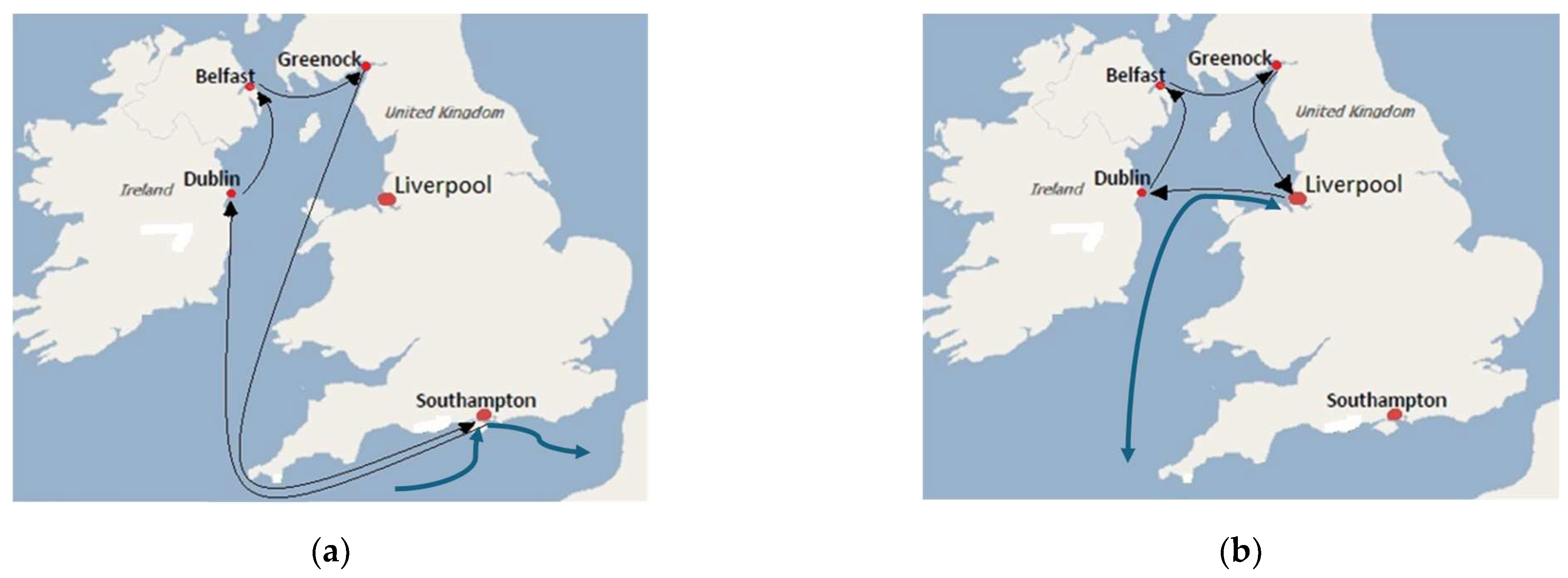
The feeder services from the Port of Southampton and from the Port of Liverpool are shown in Figure 1. The three scenarios of container shipping supply chains are illustrated in Figure 2, where Base CSSC represents Scenario 1, Regional port CSSC represents Scenario 2, and Dual port CSSC represents Scenario 3.

To evaluate the viability of rerouting the Asia–Europe shipping services to the regional port in Scenarios 2 and 3, compared to the base scenario, we exclude the hinterland transport logistics associated with the original ports (i.e., foreign ports). This is because the related costs and CO₂ emissions will be identical across all three scenarios in the segment of the supply chain from original hinterland to original ports (Figure 2).

Our analysis focuses on the costs and CO₂ emissions in the supply chain segments from the original ports to the final inland destinations, including deep-sea services, port operations, feeder services, and inland rail and road transport, as shown in Figure 2. Specifically, the scenario evaluation includes the following steps:

• Step 1. Calculate deep-sea service costs and CO₂ emissions in Section 3.2.
• Step 2. Calculate port handling costs and CO₂ emissions in Section 3.3.
• Step 3. Calculate feeder service costs and CO₂ emissions in Section 3.4.
• Step 4. Calculate inland rail and road transportation costs and CO₂ emissions in Section 3.5.
• Step 5. Obtain total relevant costs and CO₂ emissions for three scenarios and calculate the performance differences between rerouting scenarios and the base scenario in Section 3.6.

We make the following assumptions:

Assumption 1. The deep-sea shipping services and feeder services operate on a weekly schedule. The round-trip journey times for both the deep-sea service routes and feeder services are consistent across the three scenarios, which will be achieved by appropriately adjusting vessel sailing speeds in the proposed scenarios.

Assumption 2. The vessel’s port times at non-UK ports are identical across all three scenarios. In Scenario 3, the combined container handling time at Southampton and Liverpool is equal to the port handling time at Southampton in the base scenario (Scenario 1) and the port handling time at Liverpool in Scenario 2. At any specific port, container loading and unloading handling charges are identical across the three scenarios. All containers are measured in TEUs (20-foot equivalent units), with one FEU (40-foot equivalent unit) counted as two TEUs.

Assumption 3. All vessels deployed for the same service are of a similar type and size.

Assumption 4. The number of containers flowing into a port by sea is the same as the number of containers flowing out of the port by sea.

Assumption 1 implies that the same number of deep-sea vessels (and feeder vessels) are deployed across all three scenarios. Note that the total sailing distances for the round-trip journey differ in each scenario. Therefore, the sailing speeds of the vessels will vary to maintain the same journey time for a round-trip. It should be noted that the adjustments of sailing speeds will have a significant impact on fuel consumption and on CO₂ emissions. Assumption 2 is reasonable under the assumption that two ports have similar handling rates and the total loading and unloading activities (for both laden and empty containers) are very similar across scenarios. Assumption 3 is common in practice because sister vessels are often deployed on the same service route. Assumption 4 follows the common principle of container flow balancing in the literature (e.g., [29]).

3.1. Notation

We introduce the following notation:

h: the UK hinterland shipment volume in TEUs in the dominant direction.

h_i: the UK hinterland shipment volume in TEUs at inland location i, i = 1, 2, …, N, h = ∑_i h_i.

d_1i, d_2i: the distances in km from inland location i to Southampton and Liverpool, respectively, i = 1, 2,…, N.

θ_1i: the proportion of the UK hinterland shipment volume at inland location i transported by road haulers via Southampton in Scenario 1, i = 1, 2, …, N; while (1 − θ_1i) is the proportion transported by rail services in Scenario 1.

θ_2i: the proportion of the UK hinterland shipment volume at inland location i transported by road haulers via Liverpool in Scenario 2, i = 1, 2, …, N; while (1 − θ_2i) is the proportion transported by rail services in Scenario 2.

θ_3,1i, θ_3,2i: the proportions of the UK hinterland shipment volume at inland location i transported by road haulers via Southampton and Liverpool in Scenario 3, i = 1, 2, …, N.

δ_3,1i, δ_3,2i: the proportions of the UK hinterland shipment volume at inland location i transported by rail services via Southampton and Liverpool in Scenario 3, where θ_3,1i + θ_3,2i + δ_3,1i + δ_3,2i = 1, for i = 1, 2, …, N.

g: the transshipment volume in TEUs in the dominant direction.

C_h: the unit transportation cost per km in USD in the hinterland by road haulers.

C_r: the unit transportation cost per km in USD in the hinterland by rail services.

C_rt: the unit handling cost in USD at seaport rail terminal or inland rail terminal.

W₁, W₂: the terminal handling charge per TEU in USD at Southampton and Liverpool.

Y(V): the fixed vessel berthing costs per call at a port, where V represents the vessel capacity.

Z₁, Z₂: the congestion cost per TEU in USD at Southampton and Liverpool.

C_fuel: the marine fuel cost per tonne in USD.

V_d: the vessel carrying capacity in TEUs in the deep-sea service.

V_f: the vessel carrying capacity in TEUs in the feeder service.

s_d0: the designed speed in knots of the deep-sea vessels.

s_f0: the designed speed in knots of the feeder vessels.

s_d1, s_d2, s_d3: the sailing speed in knots of the deep-sea vessels in Scenarios 1, 2, and 3.

s_f1, s_f2, s_f3: the sailing speed in knots of the feeder vessels in Scenarios 1, 2 and 3.

d_d1, d_d2, d_d3: the sailing distance in nautical miles of the round-trip journey of the deep-sea service route in Scenarios 1, 2 and 3.

d_f1, d_f2, d_f3: the sailing distance in nautical miles of the round-trip journey of the feeder service route in Scenarios 1, 2 and 3.

F_d: the fuel consumption in tonnes per day when a vessel in the deep-sea service sails at its designed speed.

F_f: the fuel consumption in tonnes per day when a vessel in the feeder service sails at its designed speed.

G_d(s_dj): the fuel consumption in tonnes per day when a vessel in the deep-sea service sails at the speed s_dj.

G_f(s_fj): the fuel consumption in tonnes per day when a vessel in the feeder service sails at the speed s_fj.

K_m: the emission factor that converts the consumed marine fuel into the emissions, which represents the tonnes of CO₂ emitted per tonne of marine fuel burned by the engine.

K_w1, K_w2: the CO₂ emissions in grams per container caused by port congestion at Southampton and Liverpool, respectively.

K_rt: the CO₂ emissions in grams per container handled at seaport rail terminal or inland rail terminal.

K_h: the CO₂ emissions in grams per tonne-km (g CO₂/tkm) by road haulers.

K_r: the CO₂ emissions in grams per tonne-km (g CO₂/tkm) by rail services.

3.2. Deep-Sea Service Costs and CO₂ Emissions

The operating costs of deep-sea services primarily include vessel chartering, crew salaries, and fuel consumption. Since all three scenarios involve the same number and type of vessels with identical round-trip journey times, the chartering and crew costs remain constant and can therefore be excluded. Consequently, only fuel consumption costs need to be evaluated, as vessel speeds vary across the three scenarios. The relevant deep-sea service cost for scenario j, denoted by RC_dj, is given by

RC_dj = C_fuel · G_d(s_dj) · d_dj/(24s_dj), for j = 1, 2, 3.

(1)

Note that the deep-sea service in Scenario 2 differs from that in Scenario 1 only by replacing Southampton with Liverpool. This implies that the number of port calls and the number of container loading/unloading activities in the deep-sea service remain the same in both scenarios, although the total sailing distances in two scenarios are different. As a result, the total time a vessel spends at ports during a round trip on the deep-sea service route is identical in Scenario 1 and Scenario 2. Therefore, the sailing speeds in Scenario 2 can be determined by ensuring that the total sailing time at sea remains the same as in Scenario 1, in order to maintain the same overall round-trip duration, i.e.,

s_d2 = d_d2 · s_d1/d_d1.

(2)

The deep-sea service in Scenario 3 differs from that in Scenario 1 by adding Liverpool to the route. This change not only increases the total sailing distance but also adds additional port call time (e.g., for vessel mooring and casting off at Liverpool). We assume the additional port call time to be 8 h [4]. Consequently, the deep-sea vessel must operate at a higher sailing speed to compensate for the extra distance and time, in order to maintain the same overall round-trip duration as in Scenario 1. Based on this, the sailing speeds in Scenario 3 can be determined as follows:

s_d3 = d_d3/(d_d1/s_d1 − 8).

(3)

It is widely accepted that a vessel’s fuel consumption follows a cubic relationship with its sailing speed (e.g., [4,30]). It follows that

G_d(s_dj): = F_d · (s_dj/s_d0)³, for j = 1, 2, 3.

(4)

The CO₂ emissions can be estimated from marine fuel consumption by multiplying it by the emission factor K_m. The emission factor is an empirical mean value that depends on the specific fuel used. Hence, the relevant CO₂ emissions of a vessel in deep-sea service, RE_dj for scenario j, are given by

RE_dj = K_m · G_d(s_dj) · d_dj/(24s_dj), for j = 1, 2, 3.

(5)

3.3. Port Handling Costs and CO₂ Emissions

Three types of port handling costs will be considered: the fixed vessel berthing costs per call at a port, the terminal handling charges, and the port congestion costs.

We assume that the fixed vessel berthing costs per call at a port only depends on vessel capacity. According to Shintani et al. [31], we have Y(V) = 1.95*V + 5200. In all three scenarios, the fixed vessel berthing costs for feeder services are the same. However, for the deep-sea service, it should be noted that both Southampton and Liverpool are called in Scenario 3, where only Southampton is called in Scenario 1 and only Liverpool is called in Scenario 2.

Terminal handling charges primarily arise from quay crane operations when containers are lifted on or off vessels. Port congestion costs are associated with yard density levels and are incurred due to unproductive yard equipment activities and vehicle waiting. In the base CSSC scenario, all hinterland shipments and transshipments are unloaded from deep-sea vessels to storage yards at Southampton. According to Assumption 4, the same number of shipments and transshipments (including both laden and empty containers) will later be loaded onto deep-sea vessels. For transshipments, double handling is required due to the use of feeder vessels. Therefore, in Scenario 1, the number of handlings for hinterland shipments equals 2h containers, while the number of handlings for transshipments equals 4g. The numbers of container handlings for Scenario 2 and Scenario 3 can be analyzed similarly. Consequently, we have the relevant port handling costs in three scenarios, RC_pj for j = 1, 2, 3, as follows:

RC_p1 = Y(V_d) + Y(V_f) + (W₁ + Z₁) · (2h + 4g),

(6)

RC_p2 = Y(V_d) + Y(V_f) + (W₂ + Z₂) · (2h + 4g),

(7)

RC_p3 = 2Y(V_d) + Y(V_f) + (W₁ + Z₁) · 2h_3,1 + (W₂ + Z₂) · (2h − 2h_3,1 + 4g).

(8)

where h_3,1 = Σ_i h_i · (θ_3,1i + δ_3,1i) represents the hinterland shipment volume handled at the port of Southampton in Scenario 3.

Regarding CO₂ emissions at ports, since the total berthing time of the vessels is consistent across the three scenarios, the emissions from the vessels, primarily caused by their auxiliary engines, remain unchanged and can be excluded from the comparison. However, as two ports may experience different levels of port congestion, external trucks, yard cranes, and internal trucks may generate different amounts of CO₂ emissions when handling hinterland shipments. It is worth noting that transshipment operations at ports are less affected by yard congestion, and their emissions are therefore excluded from the analysis. We use RE_pj for j = 1, 2, 3 to denote the relevant port operations emissions as follows:

RE_p1 = K_w1 · 2h,

(9)

RE_p2 = K_w2 · 2h,

(10)

RC_p3 = K_w1 · 2h_3,1 + K_w2 · 2(h − h_3,1).

(11)

3.4. Feeder Service Costs and CO₂ Emissions

Similar to the deep-sea service cost, the feeder service costs can focus on the fuel consumption costs of feeder vessels. The relevant feeder service cost for scenario j, denoted by RC_fj, is given by

RC_fj = C_fuel · G_f(s_fj) · d_fj/(24s_fj), for j = 1, 2, 3.

(12)

where

s_fj = d_fj · s_f1/d_f1, for j = 1, 2, 3.

(13)

G_f(s_fj): = F_f · (s_fj/s_f0)³, for j = 1, 2, 3.

(14)

The relevant CO₂ emissions of a vessel in feeder service, RE_fj for scenario j, are given by

RE_fj = K_m · G_f(s_fj) · d_fj/(24s_fj), for j = 1, 2, 3.

(15)

3.5. Inland Rail and Road Transportation Costs and CO₂ Emissions

It is assumed that the UK hinterland shipments are distributed over N inland locations with {h_i: i = 1, 2, …, N; Σ_i h_i = h}. For road haulage, the containers can be delivered directly between the port and customers. However, for rail services, the containers must be handled at both seaport rail terminal and inland rail terminal, and further transported by trucks between inland rail terminals and customers. For simplicity, we assume there is an average of 30 km between inland rail terminals and customers. The relevant hinterland transportation costs by road haulers and rail services for three scenarios, denoted by RC_hj for j = 1, 2, 3, can be calculated as follows:

RC_h1 = C_h · Σ_i (θ_1i · 2h_i · d_1i) + Σ_i 2h_i· (1 − θ_1i) · (C_r·d_1i + 2C_rt + 30C_h);

(16)

RC_h2 = C_h · Σ_i (θ_2i · 2h_i · d_2i) + Σ_i 2h_i · (1 − θ_2i) · (C_r·d_2i + 2C_rt + 30C_h);

(17)

RC_h3 = C_h · Σ_i (θ_3,1i · 2h_i · d_1i + θ_3,2i · 2h_i · d_2i)
  + Σ_i 2h_i· δ_3,1i · (C_r·d_1i + 2C_rt + 30C_h) + Σ_i 2h_i· δ_3,2i · (C_r·d_2i + 2C_rt + 30C_h).

(18)

The average weight per container in both directions (to and from ports) can be estimated at 15 tonnes, considering both laden and empty containers. The CO₂ emissions per tonne-kilometer by road haulers, K_h, are approximately 106.5 g CO₂/tkm [32]. The CO₂ emissions per tonne-kilometer by rail services, K_r, are approximately 26.5 g CO₂/tkm in the UK [33]. For rail services, the emissions from container handling at both seaport rail terminal and inland rail terminal, K_rt, are about 8040 g CO₂ per container. Therefore, the relevant CO₂ emissions in tonnes from hinterland transportation by road haulers and rail services for three scenarios, denoted by RE_hj for j = 1, 2, 3, can be calculated as follows:

RE_h1 = 15K_h · Σ_i (θ_1i · 2h_i · d_1i) · 10⁻⁶ + Σ_i (1 − θ_1i)·2h_i·(15K_r ·d_1i + 2K_rt + 15K_h ·30) · 10⁻⁶;

(19)

RE_h2 = 15K_h · Σ_i (θ_2i · 2h_i · d_2i) · 10⁻⁶ + Σ_i (1 − θ_2i)·2h_i·(15K_r ·d_2i + 2K_rt + 15K_h ·30) · 10⁻⁶;

(20)

RE_h3 = 15K_h · Σ_i (θ_3,1i·2h_i·d_1i + θ_3,2i·2h_i·d_2i)·10⁻⁶ + Σ_i [δ_3,1i·2h_i·(10K_r ·d_1i + 2K_rt + 15K_h ·30)
   + δ_3,2i·2h_i·(15K_r ·d_2i + 2K_rt + 15K_h ·30)]·10⁻⁶.

(21)

3.6. Total Relevant Costs and CO₂ Emissions in Three Scenarios

In summary, the total relevant costs and CO₂ emissions in three CSSC scenarios, denoted by TRC_j and TRE_j for j = 1, 2, 3, are given by

TRC_j = RC_dj + RC_pj + RC_fj + RC_hj, for j = 1, 2, 3.

(22)

TRE_j = RE_dj + RE_pj + RE_fj + RE_hj, for j = 1, 2, 3.

(23)

Using the base CSSC scenario (i.e., Scenario 1) as the reference point, we can obtain the relative total relevant costs and CO₂ emissions between Scenarios 2 and 3 compared to Scenario 1 as follows:

TRC₂ − TRC₁ = C_fuel · F_d · s_d1² (d_d2³ − d_d1³)/(24 · d_d1² · s_d0³)
+ (W₂ + Z₂ − W₁ − Z₁) · (2h + 4g)
+ C_fuel · F_f · s_f1² (d_f2³ – d_f1³)/(24 · d_f1² · s_f0³)
+ C_h·Σ_i 2h_i·(θ_2i·d_2i − θ_1i·d_1i) + Σ_i 2h_i·C_r·[(1 − θ_2i)·d_2i − (1 − θ_1i)·d_1i]
+ Σ_i 2h_i·(θ_1i − θ_2i) · (2C_rt + 30C_h).

(24)

TRC₃ − TRC₁ = C_fuel · F_d · (s_d3²·d_d3 − s_d1²·d_d1)/(24 · s_d0³)
+ Y(V_d) + (W₂ + Z₂ − W₁ − Z₁)· (2h − 2h_3,1 + 4g)
+ C_fuel · F_f · s_f1² (d_f3³ − d_f1³)/(24 · d_f1² · s_f0³)
+ C_h·Σ_i 2h_i·(θ_3,1i·d_1i + θ_3,2i·d_2i − θ_1i·d_1i) + Σ_i 2h_i·C_r·[δ_3,1i·d_1i + δ_3,2i·d_2i − (1 − θ_1i)·d_1i]
+ Σ_i 2h_i· (δ_3,1i + δ_3,2i − 1 + θ_1i) · (2C_rt + 30C_h).

(25)

TRE₂ − TRE₁ = K_m · F_d · s_d1² (d_d2³ − d_d1³)/(24 · d_d1² · s_d0³)
+ 2h · (K_w2 − K_w1) · 10⁻⁶
+ K_m · F_f · s_f1² (d_f2³ − d_f1³)/(24 · d_f1² · s_f0³)
+ 15K_h·Σ_i 2h_i·(θ_2i·d_2i − θ_1i·d_1i) · 10⁻⁶ + ∑_i 2h_i· 15K_r·[(1 − θ_2i)·d_2i − (1 − θ_1i)·d_1i)] · 10⁻⁶
+ Σ_i 2h_i·[(θ_1i − θ_2i) · (2K_rt + 15K_h ·30)] · 10⁻⁶.

(26)

TRE₃ − TRE₁ = K_m · F_d · (s_d3²·d_d3 − s_d1²·d_d1)/(24 · s_d0³)
+ 2(h − h_3,1) · (K_w2 − K_w1) · 10⁻⁶
+ K_m · F_f · s_f1² (d_f3³ − d_f1³)/(24 · d_f1² · s_f0³)
+ 15K_h·∑_i2h_i·(θ_3,1i·d_1i + θ_3,2i·d_2i − θ_1i·d_1i) · 10⁻⁶ + Σ_i2h_i·15K_r·[δ_3,1i·d_1i + δ_3,2i·d_2i − (1 − θ_1i)·d_1i] · 10⁻⁶
+ Σ_i2h_i·[(δ_3,1i + δ_3,2i − (1 − θ_1i)) · (2K_rt + 15K_h ·30)] · 10⁻⁶.

(27)

Proposition 1.

Suppose that the major port (Southampton) has a closer proximity to maritime routes (d_d3 > d_d2 > d_d1), while the regional port (i.e., Liverpool) has a closer proximity to transshipment markets (d_f3 = d_f2 < d_f1). Additionally, the regional port (Liverpool) has lower terminal handling charges (W₁ > W₂) and lower port congestion costs (Z₁ > Z₂). Under these conditions, we have the following results regarding the relative total relevant costs:

(i)

TRC₂–TRC₁ and TRC₃–TRC₁ are increasing in s_d1 but decreasing in s_f1.

(ii)

TRC₂–TRC₁ and TRC₃–TRC₁ are decreasing in d_d1.

(iii)

TRC₂–TRC₁ and TRC₃–TRC₁ are decreasing in W₁ − W₂ and Z₁ − Z₂.

(iv)

TRC₂–TRC₁ and TRC₃–TRC₁ are decreasing in g.

The results in Proposition 1 can be derived from (24) and (25). Proposition 1(i) follows from the conditions d_d3 > d_d2 > d_d1 and d_f3 = d_f2 < d_f1. This implies that a smaller s_d1 or a larger s_f1 tends to increase the competitiveness of rerouting to Liverpool. Proposition 1(ii) implies that a longer round-trip journey distance in the base CSSC scenario tends to increase the competitiveness of rerouting to Liverpool. Proposition 1(iii) arises from the conditions W₁ > W₂ and Z₁ > Z₂. This is intuitive as lower terminal handling charges and reduced port congestion at Liverpool encourage rerouting to Liverpool. Finally, Proposition 1(iv) indicates that the volume of transshipments (g) has a positive impact on rerouting to Liverpool. This follows from the conditions W₁ > W₂ and Z₁ > Z₂.

Proposition 2.

Suppose that the major port (Southampton) has a closer proximity to maritime routes (d_d3 > d_d2 > d_d1), while the regional port (i.e., Liverpool) has a closer proximity to transshipment markets (d_f3 = d_f2 < d_f1). Additionally, the regional port (Liverpool) is less congested (K_w2 < K_w1). We have the following results regarding the relative total CO₂ emissions:

(i)

TRE₂–TRE₁ and TRE₃–TRE₁ are increasing in s_d1 but decreasing in s_f1.

(ii)

TRE₂–TRE₁ and TRE₃–TRE₁ are decreasing in d_d1.

(iii)

TRC₂–TRC₁ and TRC₃–TRC₁ are decreasing in (K_w2 − K_w1).

The results in Proposition 2 can similarly be derived from Equations (26) and (27). Notably, Propositions 2(i–iii) align with Proposition 1(i–iii), indicating that the relative costs and CO₂ emissions exhibit similar sensitivities to these factors in Proposition 2. However, the results in both Proposition 1 and Proposition 2 are qualitative. A more insightful analysis involves quantitatively evaluating these sensitivities, which will be explored in the next section.

4. Numerical Experiments and Sensitivity Analysis

The system parameters can be classified into several categories: shipping service-related, port-related, and hinterland transport-related parameters. Shipping service-related parameters are set as follows. The deep-sea vessel has capacity V_d = 10,000 TEUs with a designed speed s_d0 = 23 knots; the feeder vessel has a capacity V_f = 600 TEUs with a designed speed s_f0 = 18 knots; it is assumed that in the base scenario the feeder vessel’s sailing speed is 5 knots less than the deep-sea vessel, i.e., s_f1 = s_d1 − 5.

Biofuel, as a drop-in fuel, is considered one of the most promising low-carbon alternative fuels. In this study, we assume that both deep-sea vessels and feeder vessels operate using biofuel. The deep-sea vessel’s fuel consumption per day at designed speed F_d = 205 tonnes; the feeder vessel’s fuel consumption per day at designed speed F_f = 33 tonnes. The biofuel cost C_fuel = USD 1000/tonne. The fuel emission factor K_m = 1.2 g CO₂/g [34].

To calculate the differences in sailing distances for deep-sea services across three scenarios, we use the following Asia–Europe service route as an example, omitting several Far East ports at the beginning and end of the port rotation:

Scenario 1 (base): Far East ports–Singapore–Rotterdam–Hamburg–Southampton–Singapore–Far East ports.

Scenario 2: Far East ports–Singapore–Rotterdam–Hamburg–Liverpool–Singapore–Far East ports.

Scenario 3: Far East ports–Singapore–Liverpool–Rotterdam–Hamburg–Southampton–Singapore–Far East ports.

According to HiFleet [35], the relevant port-to-port distances in nautical miles can be obtained as follows:

• Singapore–8436–Rotterdam–314–Hamburg–521–Southampton–8214–Singapore.
• Singapore–8436–Rotterdam–314–Hamburg–903–Liverpool–8335–Singapore.
• Singapore–8335–Liverpool–706–Rotterdam–314–Hamburg–521–Southampton–8214–Singapore.

Therefore, the round-trip journey distances for the deep-sea services in Scenario 2 and Scenario 3 are 503 and 605 nautical miles longer, respectively, than in the base scenario, i.e., d_d2 = d_d1 + 503, d_d3 = d_d1 + 605. The round-trip journey distance in the feeder service in the base scenario (Southampton–583–Greenock–97–Belfast–115–Dublin–432–Southampton) is d_f1 = 1227. The round-trip journey distances in the feeder services in Scenario 2 and Scenario 3 (Liverpool feeder route: Liverpool–203–Greenock–97–Belfast–115–Dublin–134–Liverpool) are d_f2 = d_f3 = 549 nautical miles.

Port-related parameters are set as follows. Currently, Liverpool (port 2) is less congested and has a lower terminal handling charge compared to Southampton (port 1). For example, according to CMA CGM, its terminal handling charge at Liverpool is GBP 15 less than that at Southampton. We therefore assume the following: W₂ − W₁ = USD −15; Z₂ − Z₁ = USD −10; K_w2 − K_w1 = −1072 g CO₂ per container, where the last equation represents the amount of CO₂ emissions for additional 10~15 min waiting at ports for an external truck [36]. The fixed vessel berthing costs per call at a port is given by Y(V) = 1.95*V + 5200, where V represents the vessel capacity in TEUs.

Hinterland transport-related parameters are set as follows. The cost of transporting a container by truck C_h = USD 2.5/km; the cost of transporting a container by rail C_r = USD 0.3/km. However, for rail containers, it incurs handling costs at both seaport and inland rail terminals, i.e., C_rt = USD 187.5 per container at each rail terminal. In addition, the inland rail terminals are often some distance from customer locations. It is assumed that the distance between inland terminals and customers is 30 km, with deliveries made by trucks. Let K_h = 106.5 g CO₂ per tonne-km by truck; K_r = 26 g CO₂ per tonne-km by rail; K_rt = 8040 g CO₂ per container handled at rail terminals; and the average container weight is 15 tonnes [37].

According to Rodrigues et al. [38], hinterland shipment locations in the UK can be categorized into nine regions, with reference cities listed in

Table 1. Hinterland shipment distribution in the UK with distances from ports of Southampton and Liverpool in km.

Region	Reference Cities	% of TEU	Liverpool (km)	Southampton (km)
North East	Newcastle	2.98	282	526
York and Humber	Leeds and Sheffield	9.55	141	365
East Midland	Derby	29.70	156	277
East England	Northampton	8.64	242	153
South East	London	24.12	343	129
South West	Exeter	2.51	411	151
North West	Liverpool and Manchester	16.83	30	380
Wales	Swansea	1.07	391	279
Scotland	Edinburgh	4.59	354	692

. To account for the influence of the Ports of Felixstowe and London Gateway on the East of England and South East regions, we halve the shipment volumes in these two regions relative to the data from [38]. The distribution of container volumes across these locations is presented in Table 1, where the last two columns indicate the distances from the ports of Southampton and Liverpool to each location, respectively.

It is assumed that the farthest inland locations are prioritized for rail service, as it is common practice for road transport to be less competitive than rail for long-distance deliveries. In Scenario 1, the Port of Southampton has a rail-to-road modal split of 0.3:0.7, while the Port of Liverpool has a modal split of 0.1:0.9 in Scenario 2. These modal splits reflect the current practices. In Scenario 3, the modal split at both ports remains unchanged. However, hinterland regions are assigned exclusively to their nearest port: shipments closer to Liverpool route solely through Liverpool, while those nearer to Southampton use Southampton exclusively.

In the following, we will examine the impact of key system parameters (including deep-sea vessel speed s_d1, the round-trip distance in deep-sea service d_d1, the hinterland shipment volume h, the CO₂ emission factor of marine fuel K_m, the marine fuel cost per tonne C_fuel, the reduction in terminal handling charge at Liverpool W₁ − W₂, and the modal split at Liverpool modalSplit₂) on the relative costs and CO₂ emissions between Scenarios 2 and 3 and the base Scenario 1 one by one. The selections of these parameters are explained as follows. The varying deep-sea vessel speed can represent shipping companies’ different levels of slow steaming practices. The varying round-trip distance in deep-sea service represents deep-sea service’s different route structures, e.g., via Suez Canal or the Cape of Good Hope. The varying hinterland shipment volume represents the potential growth of the UK trade market. The varying CO₂ emission factors of marine fuel represent the different levels of carbon reduction for alternative fuels. The varying marine fuel cost per tonne can represent different cost scenarios of alternative ship fuels. The reduction in terminal handling charge at Liverpool can reflect the economy of scale at the port of Liverpool, i.e., as port handling volumes grow, the unit cost of handling would reduce. The rising modal share of rail transport in Liverpool shows that rail usage is increasing to levels matching those in Southampton.

The performance differences between Scenarios 2 and 3 compared to Scenario 1 in the experiments are presented in

Table 2. Performance differences between scenarios with varying deep-sea vessel speed.

	sd1	deepseaCost	portCost	feederCost	roadCost	railCost	totalCost
Scenario 2	22	522,719	−150,000	−76,115	228,155	−473,765	50,994
minus	20	431,999	−150,000	−59,259	228,155	−473,765	−22,870
Scenario 1	18	349,920	−150,000	−44,510	228,155	−473,765	−90,201
	16	276,480	−150,000	−31,868	228,155	−473,765	−150,999
	14	211,680	−150,000	−21,333	228,155	−473,765	−205,264
Scenario 3	22	760,634	−88,960	−76,115	−464,828	−340,058	−209,327
minus	20	618,806	−88,960	−59,259	−464,828	−340,058	−334,299
Scenario 1	18	493,296	−88,960	−44,510	−464,828	−340,058	−445,060
	16	383,505	−88,960	−31,868	−464,828	−340,058	−542,209
	14	288,837	–88,960	–21,333	–464,828	–340,058	–626,342
	sd1	deepseaCO2	portCO2	feederCO2	roadCO2	railCO2	totalCO2
Scenario 2	22	627.3	−4.3	−91.3	145.8	−199.1	478.3
minus	20	518.4	−4.3	−71.1	145.8	−199.1	389.7
Scenario 1	18	419.9	−4.3	−53.4	145.8	−199.1	308.9
	16	331.8	−4.3	−38.2	145.8	−199.1	235.9
	14	254.0	−4.3	−25.6	145.8	−199.1	170.8
Scenario 3	22	912.8	−2.7	−91.3	−297.0	−176.9	344.7
minus	20	742.6	−2.7	−71.1	−297.0	−176.9	194.8
Scenario 1	18	592.0	−2.7	−53.4	−297.0	−176.9	61.9
	16	460.2	−2.7	−38.2	−297.0	−176.9	−54.7
	14	346.6	–2.7	–25.6	–297.0	–176.9	–155.7

,

Table 3. Performance differences between scenarios with varying round-trip distance in deep-sea service.

	dd1	deepseaCost	portCost	feederCost	roadCost	railCost	totalCost
Scenario 2	22,000	351,144	−150,000	−44,510	228,155	−473,765	−88,976
minus	24,000	350,480	−150,000	−44,510	228,155	−473,765	−89,640
Scenario 1	26,000	349,920	−150,000	−44,510	228,155	−473,765	−90,201
	28,000	349,439	−150,000	−44,510	228,155	−473,765	−90,681
	30,000	349,024	−150,000	−44,510	228,155	−473,765	−91,097
Scenario 3	22,000	496,063	−88,960	−44,510	−464,828	−340,058	−442,294
minus	24,000	494,562	−88,960	−44,510	−464,828	−340,058	−443,794
Scenario 1	26,000	493,296	−88,960	−44,510	−464,828	−340,058	−445,060
	28,000	492,213	−88,960	−44,510	−464,828	−340,058	−446,143
	30,000	491,277	−88,960	−44,510	−464,828	−340,058	−447,080
	dd1	deepseaCO2	portCO2	feederCO2	roadCO2	railCO2	totalCO2
Scenario 2	22,000	421.4	−4.3	−53.4	145.8	−199.1	310.4
minus	24,000	420.6	−4.3	−53.4	145.8	−199.1	309.6
Scenario 1	26,000	419.9	−4.3	−53.4	145.8	−199.1	308.9
	28,000	419.3	−4.3	−53.4	145.8	−199.1	308.3
	30,000	418.8	−4.3	−53.4	145.8	−199.1	307.8
Scenario 3	22,000	595.3	−2.7	−53.4	−297.0	−176.9	65.2
minus	24,000	593.5	−2.7	−53.4	−297.0	−176.9	63.4
Scenario 1	26,000	592.0	−2.7	−53.4	−297.0	−176.9	61.9
	28,000	590.7	−2.7	−53.4	−297.0	−176.9	60.6
	30,000	589.5	–2.7	–53.4	–297.0	–176.9	59.4

,

Table 4. Performance differences between scenarios with varying hinterland shipment volume.

	h	deepseaCost	portCost	feederCost	roadCost	railCost	totalCost
Scenario 2	2000	349,920	−150,000	−44,510	228,155	−473,765	−90,201
minus	2500	349,920	−175,000	−44,510	285,194	−592,206	−176,603
Scenario 1	3000	349,920	−200,000	−44,510	342,233	−710,647	−263,006
	3500	349,920	−225,000	−44,510	399,271	−829,089	−349,408
Scenario 3	2000	493,296	−88,960	−44,510	−464,828	−340,058	−445,060
minus	2500	493,296	−104,875	−44,510	−581,035	−425,072	−662,197
Scenario 1	3000	493,296	−120,790	−44,510	−697,242	−510,087	−879,333
	3500	493,296	–136,705	–44,510	–813,449	–595,101	–1,096,470
	h	deepseaCO2	portCO2	feederCO2	roadCO2	railCO2	totalCO2
Scenario 2	2000	419.9	−4.3	−53.4	145.8	−199.1	308.9
minus	2500	419.9	−5.4	−53.4	182.2	−248.9	294.5
Scenario 1	3000	419.9	−6.4	−53.4	218.7	−298.7	280.1
	3500	419.9	−7.5	−53.4	255.1	−348.4	265.7
Scenario 3	2000	592.0	−2.7	−53.4	−297.0	−176.9	61.9
minus	2500	592.0	−3.4	−53.4	−371.3	−221.2	−57.3
Scenario 1	3000	592.0	−4.1	−53.4	−445.5	−265.4	−176.5
	3500	592.0	–4.8	–53.4	–519.8	–309.6	–295.7

,

Table 5. Performance differences between scenarios with varying marine-fuel emission factor.

	Km	deepseaCost	portCost	feederCost	roadCost	railCost	totalCost
Scenario 2	1.20	349,920	−150,000	−44,510	228,155	−473,765	−90,201
minus	1.00	349,920	−150,000	−44,510	228,155	−473,765	−90,201
Scenario 1	0.80	349,920	−150,000	−44,510	228,155	−473,765	−90,201
	0.60	349,920	−150,000	−44,510	228,155	−473,765	−90,201
Scenario 3	1.20	493,296	−88,960	−44,510	−464,828	−340,058	−445,060
minus	1.00	493,296	−88,960	−44,510	−464,828	−340,058	−445,060
Scenario 1	0.80	493,296	−88,960	−44,510	−464,828	−340,058	−445,060
	0.60	493,296	−88,960	−44,510	−464,828	−340,058	−445,060
	Km	deepseaCO2	portCO2	feederCO2	roadCO2	railCO2	totalCO2
Scenario 2	1.20	419.9	−4.3	−53.4	145.8	−199.1	308.9
minus	1.00	349.9	−4.3	−44.5	145.8	−199.1	247.8
Scenario 1	0.80	279.9	−4.3	−35.6	145.8	−199.1	186.7
	0.60	210.0	−4.3	−26.7	145.8	−199.1	125.7
Scenario 3	1.20	592.0	−2.7	−53.4	−297.0	−176.9	61.9
minus	1.00	493.3	−2.7	−44.5	−297.0	−176.9	−27.9
Scenario 1	0.80	394.6	−2.7	−35.6	−297.0	−176.9	−117.7
	0.60	296.0	–2.7	–26.7	–297.0	–176.9	–207.4

,

Table 6. Performance differences between three scenarios with varying marine fuel unit cost.

	Cfuel	deepseaCost	portCost	feederCost	roadCost	railCost	totalCost
Scenario 2	1000	349,920	−150,000	−44,510	228,155	−473,765	−90,201
minus	900	314,928	−150,000	−40,059	228,155	−473,765	−120,742
Scenario 1	800	279,936	−150,000	−35,608	228,155	−473,765	−151,283
	700	244,944	−150,000	−31,157	228,155	−473,765	−181,823
Scenario 3	1000	493,296	−88,960	−44,510	−464,828	−340,058	−445,060
minus	900	443,966	−88,960	−40,059	−464,828	−340,058	−489,939
Scenario 1	800	394,637	−88,960	−35,608	−464,828	−340,058	−534,818
	700	345,307	−88,960	−31,157	−464,828	−340,058	−579,696
	Cfuel	deepseaCO2	portCO2	feederCO2	roadCO2	railCO2	totalCO2
Scenario 2	1000	419.9	−4.3	−53.4	145.8	−199.1	308.9
minus	900	419.9	−4.3	−53.4	145.8	−199.1	308.9
Scenario 1	800	419.9	−4.3	−53.4	145.8	−199.1	308.9
	700	419.9	−4.3	−53.4	145.8	−199.1	308.9
Scenario 3	1000	592.0	−2.7	−53.4	−297.0	−176.9	61.9
minus	900	592.0	−2.7	−53.4	−297.0	−176.9	61.9
Scenario 1	800	592.0	−2.7	−53.4	−297.0	−176.9	61.9
	700	592.0	–2.7	–53.4	–297.0	–176.9	61.9

,

Table 7. Performance differences between scenarios with varying THC reduction at Liverpool.

	W1 − W2	deepseaCost	portCost	feederCost	roadCost	railCost	totalCost
Scenario 2	15	349,920	−150,000	−44,510	228,155	−473,765	−90,201
minus	20	349,920	−180,000	−44,510	228,155	−473,765	−120,201
Scenario 1	25	349,920	−210,000	−44,510	228,155	−473,765	−150,201
	30	349,920	−240,000	−44,510	228,155	−473,765	−180,201
Scenario 3	15	493,296	−88,960	−44,510	−464,828	−340,058	−445,060
minus	20	493,296	−111,692	−44,510	−464,828	−340,058	−467,792
Scenario 1	25	493,296	−134,424	−44,510	−464,828	−340,058	−490,524
	30	493,296	−157,156	−44,510	−464,828	−340,058	−513,256
	W1 − W2	deepseaCO2	portCO2	feederCO2	roadCO2	railCO2	totalCO2
Scenario 2	15	419.9	−4.3	−53.4	145.8	−199.1	308.9
minus	20	419.9	−4.3	−53.4	145.8	−199.1	308.9
Scenario 1	25	419.9	−4.3	−53.4	145.8	−199.1	308.9
	30	419.9	−4.3	−53.4	145.8	−199.1	308.9
Scenario 3	15	592.0	−2.7	−53.4	−297.0	−176.9	61.9
minus	20	592.0	−2.7	−53.4	−297.0	−176.9	61.9
Scenario 1	25	592.0	−2.7	−53.4	−297.0	−176.9	61.9
	30	592.0	–2.7	–53.4	–297.0	–176.9	61.9

and

Table 8. Performance differences between scenarios with varying modal-split at Liverpool.

	modalSplit2	deepseaCost	portCost	feederCost	roadCost	railCost	totalCost
Scenario 2	0.1	349,920	−150,000	−44,510	228,155	−473,765	−90,201
minus	0.2	349,920	−150,000	−44,510	−114,845	−252,605	−212,041
Scenario 1	0.3	349,920	−150,000	−44,510	−457,845	−31,445	−333,881
Scenario 3	0.1	493,296	−88,960	−44,510	−464,828	−340,058	−445,060
minus	0.2	493,296	−88,960	−44,510	−579,305	−211,751	−431,230
Scenario 1	0.3	493,296	−88,960	−44,510	−678,599	−85,265	−404,039
	modalSplit2	deepseaCO2	portCO2	feederCO2	roadCO2	railCO2	totalCO2
Scenario 2	0.1	419.9	−4.3	−53.4	145.8	−199.1	308.9
minus	0.2	419.9	−4.3	−53.4	−73.4	−120.0	168.8
Scenario 1	0.3	419.9	−4.3	−53.4	−292.6	−40.9	28.8
Scenario 3	0.1	592.0	−2.7	−53.4	−297.0	−176.9	61.9
minus	0.2	592.0	−2.7	−53.4	−370.2	−142.8	22.9
Scenario 1	0.3	592.0	–2.7	–53.4	–433.6	–111.0	–8.8

. Specifically, the last columns in Table 2, Table 3, Table 4, Table 5, Table 6, Table 7 and Table 8 give the total relevant costs or CO₂ emissions of Scenario 2 and Scenario 3 minus that of Scenario 1, i.e., TRC₂–TRC₁, or TRC₃–TRC₁, or TRE₂–TRE₁, or TRE₃–TRE₁. Negative numbers in Table 2, Table 3, Table 4, Table 5, Table 6, Table 7 and Table 8 indicate the rerouting scenarios outperform the base scenario. The experiments below also demonstrate the sensitivity of the performance differences to those key parameters. Following the sensitivity analysis, the managerial insights and policy implications on the viability of rerouting to regional ports are summarized in Section 4.8.

4.1. Sensitivity of Performance Differences to the Deep-Sea Vessel Speed

In this subsection, the deep-sea vessel’s sailing speed s_d1 varies from 22, 20, 18, 16, to 14 knots. Lower speeds represent the slower steaming practices that shipping lines may adopt in response to the IMO’s decarbonization requirements. Other parameters are fixed as follows: d_d1 = 26,000, h = 2000, K_m = 1.2, C_fuel = 1000, W₁ − W₂ = 15, modalSplit₂ = 0.1. Table 2 gives the performance differences between Scenarios 2 and 3 compared to Scenario 1 for individual cost components, total relevant cost, individual CO₂ emission components, and total relevant CO₂ emissions. To visualize the trend with respect to deep-sea vessel speed more intuitively, the total cost differences (i.e., TRC₂−TRC₁, TRC₃−TRC₁) are shown in Figure 3a, and the total emission differences (i.e., TRE₂−TRE₁, TRE₃−TRE₁) are shown in Figure 3b.

Table 2 and Figure 3a show that as the deep-sea vessel speed in the base scenario decreases, the total relevant cost and CO₂ emissions for Scenarios 2 and 3 compared to the base scenario also decrease. This observation supports Proposition 1(i) and Proposition 2(i). The results indicate that slower steaming practices would favor rerouting to regional ports from both economic and emissions perspectives.

Economically, the base scenario is more favorable than Scenario 2 when s_d1 is 22 knots. However, Scenario 2 outperforms the base scenario when s_d1 is 20 knots or less. This is because extra slow steaming reduces marine fuel costs, making the deviation of the Asia–Europe route to Liverpool economically viable. Scenario 3 outperforms the base scenario for all sailing speeds in the experiments.

From the emissions perspective, Table 2 and Figure 3b show that the base scenario outperforms Scenario 2 in all sailing speeds, emitting 170 to 478 tonnes less CO₂. It also outperforms Scenario 3 when s_d1 is 18 knots or above. However, Scenario 3 outperforms the base scenario at s_d1 = 16 knots or less. In Scenario 2, the Asia–Europe service route calls at Liverpool instead of Southampton. The results in Table 2 indicate that this rerouting option would increase emissions from deep-sea services and road transport while reducing emissions from port operations, feeder services, and rail transport. However, the increase in deep-sea and road transport emissions outweighs the decreases in other areas, resulting in an overall increase in total CO₂ emissions across the entire CSSC. The increase in road transport emissions and the decrease in rail transport emissions are partially due to the significantly lower percentage of rail transport usage at Liverpool. Note that Liverpool’s rail modal shift is only 10%, compared to Southampton’s 30%. In contrast, in Scenario 3, where the Asia–Europe service route calls at both Liverpool and Southampton, the CO₂ emissions from ports, feeder services, road transport, and rail transport are all lower than that in the base scenario, except for the deep-sea service emissions.

4.2. Sensitivity of Performance Differences to the Round-Trip Distance in Deep-Sea Service

In this subsection, the round-trip journey distance for the deep-sea service d_d1 varies from 22,000, 24,000, 26,000, 28,000 and 30,000 nautical miles. Lower distances represent shipping routes via Suez Canal; higher distances represent shipping routes via Cape of Good Hope. Other parameters are fixed as follows: s_d1 = 18, h = 2000, K_m = 1.2, C_fuel = 1000, W₁ − W₂ = 15, modalSplit₂ = 0.1. Table 3 gives the performance differences between Scenarios 2 and 3 compared to Scenario 1 for individual cost components, total relevant cost, individual CO₂ emission components, and total relevant CO₂ emissions. To visualize the sensitivity of the performance differences to deep-sea route round-trip distance more intuitively, the total cost differences (i.e., TRC₂−TRC₁, TRC₃−TRC₁) are shown in Figure 4a, and the total emission differences (i.e., TRE₂−TRE₁, TRE₃−TRE₁) are shown in Figure 4b.

Table 3 shows that as the round-trip journey distance in the base scenario increases, the total relevant costs and CO₂ emissions for Scenarios 2 and 3 compared to the base scenario decrease. This observation supports Proposition 1(ii) and Proposition 2(ii). However, the impacts are minor as shown in Figure 4. This indicates that the relative performances between scenarios are less sensitive to the deep-sea route round-trip distance. In all cases, both Scenario 2 and Scenario 3 outperform the base scenario economically but underperform the base scenario in terms of CO₂ emissions. The rerouting Scenario 3 is significantly better than the rerouting Scenario 2 both economically and environmentally.

4.3. Sensitivity of Performance Differences to the Hinterland Shipment Volume

In this subsection, the hinterland shipment volume h varies from 2000, 2500, 3000, to 3500 TEUs. Other parameters are fixed as follows: s_d1 = 18, d_d1 = 26,000, K_m = 1.2, C_fuel = 1000, W₁ − W₂ = 15, modalSplit₂ = 0.1. Table 4 gives the performance differences between Scenarios 2 and 3 compared to Scenario 1 for individual cost components, total relevant cost, individual CO₂ emission components, and total relevant CO₂ emissions. The total cost differences (i.e., TRC₂−TRC₁, TRC₃−TRC₁) are visualized in Figure 5a, and the total emission differences (i.e., TRE₂−TRE₁, TRE₃−TRE₁) are shown in Figure 5b.

It can be observed from Table 4 and Figure 5 that, as the volume of hinterland shipments increases, the total relevant costs and CO₂ emissions for Scenario 2 and Scenario 3 compared to the base scenario are decreasing, while the performance difference between Scenario 3 and the base scenario is significantly more sensitive than that between Scenario 2 and Scenario 1. A higher hinterland shipment volume would favor rerouting to regional ports from both economic and emissions perspectives.

Economically, both Scenario 2 and Scenario 3 outperform the base scenario in all cases. However, from the emission perspective, the base scenario outperforms Scenario 2 in all cases. In contrast, Scenario 3 outperforms the base scenario environmentally when hinterland shipment volume increases to 2500 TEUs or above.

4.4. Sensitivity of Performance Differences to Marine-Fuel Emission Factor

In this subsection, the marine-fuel emission factor K_m varies from 1.2, 1.0, 0.8, to 0.6 gCO₂/g, representing different levels of carbon emissions from low-carbon fuels. Other parameters are fixed as follows: s_d1 = 18, d_d1 = 26,000, h = 2000, C_fuel = 1000, W₁ − W₂ = 15, modalSplit₂ = 0.1. Table 2 gives the performance differences between Scenarios 2 and 3 compared to Scenario 1 for individual cost components, total relevant cost, individual CO₂ emission components, and total relevant CO₂ emissions. The total emission differences (i.e., TRE₂−TRE₁, TRE₃−TRE₁) are visualized in Figure 6.

From Table 5, it can be observed that as the marine-fuel emission factor decreases, the cost differences between the rerouting scenarios and the base scenario remain unchanged; Scenarios 2 and 3 are consistently more economically favorable than the base scenario across all cases. From an emissions perspective, the emission difference decreases as the marine-fuel emission factor decreases (Table 5 and Figure 6). This indicates that a lower marine fuel emission factor would favor rerouting to regional ports from an emissions perspective. The base scenario outperforms Scenario 2 in all cases. In contrast, Scenario 3 becomes environmentally preferable to the base scenario when the emission factor drops to 1.0 or below.

4.5. Sensitivity of Performance Differences to Marine-Fuel Unit Cost

In this subsection, the marine-fuel unit cost C_fuel varies from 1000, 900, 800, to 700 USD/ton. Lower unit costs represent that low-carbon alternative fuels might become cheaper as they scale up in the future. Other parameters are fixed as follows: s_d1 = 18, d_d1 = 26,000, h = 2000, K_m = 1.2, W₁ − W₂ = 15, modalSplit₂ = 0.1. Table 6 gives the performance differences between Scenarios 2 and 3 compared to Scenario 1 for individual cost components, total relevant cost, individual CO₂ emission components, and total relevant CO₂ emissions. The total cost differences (i.e., TRC₂−TRC₁, TRC₃−TRC₁) are visualized in Figure 7.

As the marine-fuel unit cost decreases, the cost differences between the rerouting scenarios and the base scenario decrease (Table 6 and Figure 7), while the emission differences remain unchanged (Table 6). This indicates that a lower marine-fuel unit cost would favor rerouting to regional ports from an economic perspective. Both Scenario 2 and Scenario 3 are more economically favorable than the base scenario in all tested cases. From an emissions perspective, the base scenario outperforms both Scenarios 2 and 3 in all cases.

4.6. Sensitivity of Performance Differences to THC Reduction at Liverpool

In this subsection, the terminal handling charge reduction at Liverpool W₁ − W₂ varies from 15, 20, 25, to 30 USD/TEU. The reduction in THC at Liverpool can reflect the economy of scale at the port of Liverpool, i.e., as port handling volumes grow due to rerouting, the unit cost of handling would reduce. Other parameters are fixed as follows: s_d1 = 18, d_d1 = 26,000, h = 2000, K_m = 1.2, C_fuel = 1000, modalSplit₂ = 0.1. Table 7 gives the performance differences between Scenarios 2 and 3 compared to Scenario 1 for individual cost components, total relevant cost, individual CO₂ emission components, and total relevant CO₂ emissions. In addition, the total cost differences (i.e., TRC₂−TRC₁, TRC₃−TRC₁) are visualized in Figure 8.

As the THC reduction at Liverpool increases, the cost differences between the rerouting scenarios and the base scenario decrease (Table 7 and Figure 8), while the emission differences remain unchanged (Table 7). This indicates that a higher THC reduction at Liverpool would favor rerouting to regional ports from an economic perspective. Economically, both Scenarios 2 and 3 are more favorable than the base scenario in all cases. On the other hand, from an emissions perspective, the base scenario outperforms both Scenarios 2 and 3 in all cases.

4.7. Sensitivity of Performance Differences to Modal-Split at Liverpool

In this subsection, the rail modal rate modalSplit₂ varies from 0.1, 0.2, to 0.3. Low level 0.1 represents the current situation at Liverpool, while high level 0.3 represents the current situation at Southampton. Other parameters are fixed as follows: s_d1 = 18, d_d1 = 26,000, h = 2000, K_m = 1.2, C_fuel = 1000, W₁ − W₂ = 15. Table 8 gives the performance differences between Scenarios 2 and 3 compared to Scenario 1 for individual cost components, total relevant cost, individual CO₂ emission components, and total relevant CO₂ emissions. The total cost differences (i.e., TRC₂−TRC₁, TRC₃−TRC₁) are visualized in Figure 9a, and the total emission differences (i.e., TRE₂−TRE₁, TRE₃−TRE₁) are shown in Figure 9b.

It can be observed from Table 8 and Figure 9 that, economically, as the rail usage at Liverpool increases towards the level at Southampton, the relative total relevant cost between Scenario 2 and the base scenario decreases, while the relative total relevant cost between Scenario 3 and the base scenario slightly increases. Both Scenario 2 and Scenario 3 significantly outperform the base scenario in all cases. From the emission perspective, as the rail usage at Liverpool increases towards the level at Southampton, the relative total relevant emissions between Scenarios 2 and 3 compared to the base scenario are decreasing. The base scenario outperforms the rerouting scenarios in all cases except the case when the rail usage at Liverpool matches the level at Southampton under Scenario 3. In general, a higher rail usage at Liverpool would favor rerouting to regional ports from both economic and emissions perspectives.

4.8. Managerial Insights and Policy Implications: Viability of Rerouting to Regional Ports

Key findings under baseline parameters

The following parameter setting reflects near-current operations: deep-sea vessel speed s_d1 = 18 knots, the round-trip distance in deep-sea service d_d1 = 26,000 nautical miles, the hinterland shipment volume h = 2000 TEUs, the CO₂ emission factor of marine fuel K_m = 1.2 gCO₂/g, the marine fuel cost per tonne C_fuel = 1000 USD/ton, the reduction in terminal handling charge at Liverpool W₁ − W₂ = 15 USD/TEU, and the modal split at Liverpool modalSplit₂ = 0.1. Under this parameter setting, the key findings include the following:

• Economic viability: Rerouting to Liverpool yields significant cost savings under both scenarios, saving USD 90,201 in Scenario 2 and USD 445,060 in Scenario 3. This confirms commercial viability under current market conditions.
• Environmental trade-off: Rerouting increases total supply chain CO₂ emissions by 309 tonnes and 62 tonnes more for Scenario 2 and Scenario 3, respectively. This creates a cost–emissions trade-off for decision-makers.

Strategic levers for enhancing rerouting viability

Slower steaming practices, higher hinterland shipment volume, and increasing rail usage at Liverpool have a significant positive impact on the competitiveness of regional ports, both economically and environmentally. This implies that extra slowing steaming, increasing hinterland shipment volume, and increasing rail modal shift would favor rerouting to regional ports from both economic and emissions perspectives.

The use of alternative marine fuels with lower carbon emission factors would favor rerouting to regional ports from an emissions perspective. This implies that as near or net zero marine fuels are adopted in the future, rerouting to regional ports tends to be more favorable environmentally.

Decreasing marine-fuel unit cost or reducing terminal handling charge at Liverpool will favor rerouting to Liverpool from an economic perspective.

The relative performances between the rerouting scenarios and the base scenario are less sensitive to the deep-sea route round-trip distance. A longer distance of the deep-sea service route has a minor positive impact on the competitiveness of regional ports, both economically and environmentally.

The above findings can be summarized in

Table 9. Key factors influencing costs and emissions of rerouting to Liverpool.

Factor	Economic Impact on Rerouting	Environmental Impact on Rerouting
Slower steaming	Positive	Positive
Higher hinterland volume	Positive	Positive
Increased rail use at Liverpool	Positive	Positive
Lower fuel emission factor	Neutral	Positive
Lower fuel unit cost	Positive	Neutral
Lower THC at Liverpool	Positive	Neutral
Longer deep-sea route distance	Minor Positive	Minor Positive

.

Managerial and policy recommendations

Prioritize dual-benefit levers: Investing in rail infrastructure, incentivizing slower steaming, and fostering hinterland cargo consolidation can improve both cost and emissions performance simultaneously.

Accelerate greener fuel adoption: Policy support (subsidies, mandates) for near-zero emission marine fuels is essential to resolve the emissions trade-off and make rerouting environmentally sustainable.

Optimize port economics: Regional ports should strategically improve efficiency and offer competitive terminal handling charges to attract deep-sea services.

Implement a consolidated UK service model: An alternative rerouting scenario can be designed by introducing a rotating call pattern alternating between Southampton and Liverpool on a single Asia–Europe service. This new alternative is highly likely to be both economically and environmentally viable, allowing UK hinterland shipments to be consolidated and served more efficiently based on their proximity to these two ports. However, this scenario implies that shippers will be served bi-weekly rather than weekly.

5. Conclusions

This paper adopts a container shipping supply chain perspective to analyze the total costs and CO₂ emissions, and to evaluate the economic and environmental viability of rerouting shipping services to call at regional or secondary container ports in the era of adopting low-carbon alternative fuels. The Port of Liverpool and Asia–Europe service routes are used as a case study. The main contributions and managerial insights of this study are summarized as follows:

• We present a straightforward and practical approach based on scenario analysis to evaluate the viability of rerouting shipping services to regional or secondary ports from a container shipping supply chain perspective. This scenario-based analysis approach is broadly applicable to regional and secondary ports beyond the case study and is easy for shipping lines to implement, enabling incremental adjustments to their existing service routes. For example, our analysis is based on the use of biofuel, and it can be easily extended to other alternative fuels such as LNG and methanol.
• The results reveal that shipping lines’ slow steaming practices, the hinterland shipment volume, and the modal shift at regional ports can significantly influence the competitiveness of regional ports, both economically and environmentally.
• Two rerouting options are compared to the base scenario in the case study. The first option (Scenario 2) involves replacing Southampton with Liverpool in the Asia–Europe service routes. The second option (Scenario 3) adjusts the Asia–Europe service routes to call at both Liverpool and Southampton. The experiments show that both rerouting scenarios are economically viable in all tested cases except for one case (where s_d1 = 22 knots in Scenario 2). From the emissions perspective, Scenario 2 is not viable in all tested cases, while Scenario 3 becomes environmentally viable when the deep-sea vessel speed is less than 16 knots, or the hinterland shipment volume reaches 2500 TEUs, or the marine-fuel emission factor is less than 1.0, or Liverpool’s rail usage matches Southampton’s level. Combining these factors would further enhance Scenario 3′s environmental viability relative to the base scenario.
• A two-port strategy, either in the form of Scenario 3 or by alternating calls between Southampton and Liverpool, is a preferable rerouting option. Such a strategy would offer more economic benefits than Scenario 2 and is likely to achieve environmental benefits compared to the base scenario. This may explain recent industrial practices, such as MSC launching a new Asia–Europe service route (termed the Britannia Service) that simultaneously calls at Liverpool and London Gateway, which started in July 2024. It also aligns with the views of some UK retailers who are urging shipping lines to adopt a two-port strategy—calling at both northern and southern ports—to save costs and reduce emissions [39].

It should be noted that this study has several implications that require further research. Firstly, the hinterland shipment distribution is based on the entire UK container import market across all shipping service routes [38], which may not accurately represent the Asia–Europe shipping route. Secondly, our inland container transport analysis relies on rail–road modal splits of 0.3:0.7 at Southampton and 0.1:0.9 at Liverpool. In practice, ports may implement incentive schemes to encourage a modal shift towards rail. For example, Southampton increased the share of rail freight from 21% to 30% through the launch of the Modal Shift Programme in September 2023, offering a GBP 70 subsidy for each container transported by rail within a range of 225 km. It is plausible that other ports may introduce similar schemes. The impact of such incentives on shipping service rerouting warrants further investigation. Thirdly, greater granularity in data would enable a more accurate comparison between different scenarios, e.g., inland container transportation between ports and customers, and port handling times. Fourthly, our study adopts scenario-based analysis; it does not involve advanced optimization of ship routing and scheduling, fleet deployment, and alternative fuel selection [40]. Further research could be conducted in this direction.