A Multi-Stage Approach for External Trucks and Yard Cranes Scheduling with CO₂ Emissions Considerations in Container Terminals

Abstract

Background: In container terminals, optimizing the scheduling of external trucks and yard cranes is crucial as it directly impacts the truck turnaround time, which is one of the most critical performance measures. Furthermore, proper scheduling of external trucks contributes to reducing ${\mathrm{CO}}_2$ emissions. Methods: This paper proposes a new approach based on a mixed integer programming model to schedule external trucks and yard cranes with the objective of minimizing ${\mathrm{CO}}_2$ emissions and reducing truck turnaround time, the gap between trucking companies’ preferred arrival time and appointed time, and the energy consumption of yard cranes. The proposed approach combines data analysis and operations research techniques. Specifically, it employs a K-means clustering algorithm to reduce the number of necessary truck trips for container handling. Additionally, a two-stage mathematical model is applied. The first stage employs a bi-objective mathematical model to plan the arrival of external trucks at the terminal gates. The second stage involves a mathematical model that schedules yard cranes’ movements between different yard blocks. Results: The results show that implementing this methodology in a hypothetical case study may lead to a substantial daily reduction of approximately 31% in ${\mathrm{CO}}_2$ emissions. Additionally, the results provide valuable insights into the trade-off between satisfying the trucking companies’ preferred arrival time and the total turnaround time. Conclusions: The integration of data clustering with mathematical modeling demonstrates a notable reduction in emissions, underscoring the viability of this strategy in promoting sustainability in port-related activities.

1. Introduction

In today’s globalized world, containerized trade has become the cornerstone of the global supply chain, as vessels deliver over 80% of world trade [1]. Using containers facilitates cargo loading and unloading operations, minimizes transit times, and reduces delays. Due to the substantial expansion in maritime transportation, container terminals (CTs) face multiple challenges, such as congestion, resource capacity limitations, and environmental sustainability concerns. Accordingly, planning the different operations at CTs has gained considerable attention from both practice and academic communities.

Any container terminal consists of three main areas: (1) Seaside, where vessels are landed and loaded/unloaded by the quay cranes. (2) Yard areas, where export and import containers are temporarily stored. (3) Landsides, through which the containers are transported to/from the hinterland.

Various transportation modes are employed to transport containers between the CTs and the hinterland, such as trucks and railways. A large portion of containers are carried using external trucks (ETs) owned by different trucking companies (TCs). Each trucking company (TC) has a preferred pick-up/delivery schedule according to customer preferences. The fact that each TC operates independently and follows its own schedule raises the probability of multiple ETs arriving at the CTs during the same time window (TW), leading to congestion at the terminal gates and increased port-related emissions.

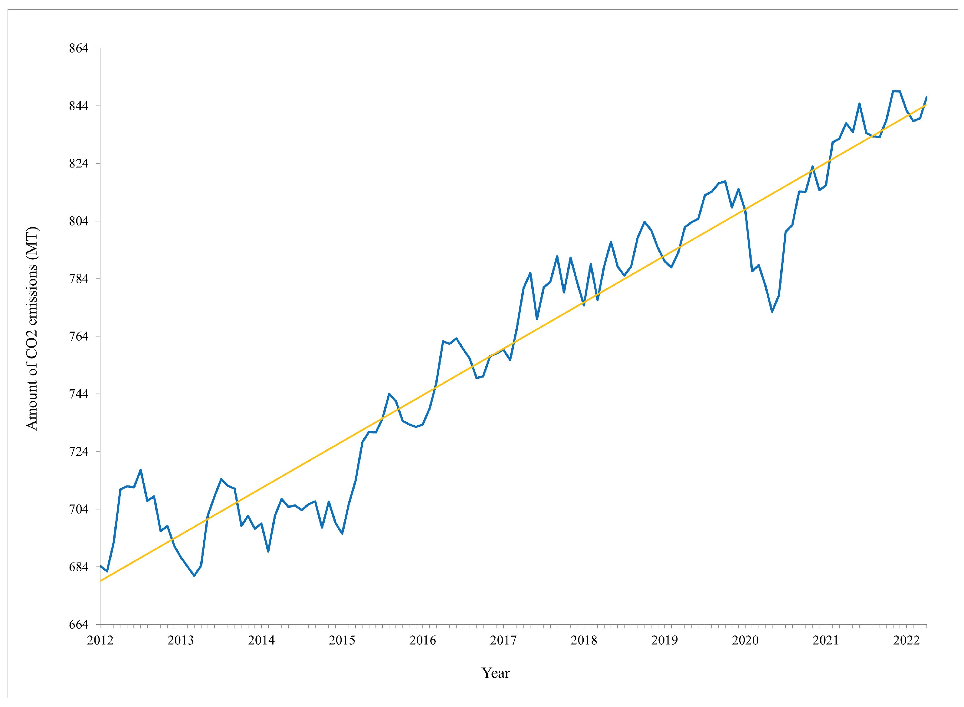
Figure 1 demonstrates the concerning trend of the increasing ${\mathrm{CO}}_2$ emissions caused by the global maritime fleet, which increased by 4.7% from 2020 to 2021. In the era of environmental sustainability, port authorities face stringent government regulations regarding the amount of ${\mathrm{CO}}_2$ emissions. These challenges require container terminals to adapt and implement innovative solutions to avoid congestion, optimize operations, and improve equipment efficiency (e.g., yard cranes, quay cranes, etc.).

To mitigate the negative impacts of terminal congestion, many container terminals developed an information-driven solution known as truck appointment systems (TAS), in which CTs offer a certain number of appointments based on the capacity of the available resources, and the TCs have the opportunity to book their appointment before visiting the terminal gates. Although implementing TAS may balance the number of arrivals over all time windows, it only solves half of the problem, as many ETs visit the terminal to pick up/deliver only one container (i.e., an empty trip).

In addition, yard cranes consume a substantial amount of energy during container handling operations due to the continuous movement between the blocks in the yard area. Accordingly, scheduling the yard crane movements efficiently saves energy and reduces port-related ${\mathrm{CO}}_2$ emissions.

This research seeks to answer the fundamental research question: “How can a TAS incorporate Data Analysis (DA) with Operations Research (OR) to enable the simultaneous reduction in empty truck trips, turnaround time, and energy consumption at container terminals?”.

In this regard, this work proposes an integrated framework to control the ETs flow to the terminal gates and schedule the yard crane operations considering the trade-off between the turnaround time and the deviation from the TCs’ preferred pick-up TW while minimizing the number of empty trips and the yard cranes total moving energy consumption. The proposed approach comprises three steps: (1) Analyzing and clustering container data using a K-means clustering algorithm to match the export and import containers based on multiple predefined criteria. (2) The results of the clustering phase are fed into a bi-objective optimization model to minimize the total turnaround time and the deviation between TC’s preferred arrival and the assigned TW. (3) Based on the ETs’ appointment schedules, the resulting workload is fed into a yard crane scheduling model to minimize the total moving energy consumption.

The primary motivation for this work is to develop efficient schedules for external trucks’ arrivals and yard cranes’ dispatching in container terminals. Among the numerous key performance indicators (KPIs) used to assess terminal performance, the turnaround time stands out as one of the most critical measures. It directly influences the performance of both container terminals and trucking companies, making it a key determinant of overall efficiency and customer satisfaction. Therefore, efficient terminal operations and swift turnaround times offer numerous advantages, such as heightened throughput, reduced congestion, and reduced waiting times for vessels, enhancing the terminal’s appeal to shipping lines and cargo owners.

The main contribution of this work is introducing a solution approach that combines the K-means clustering technique and a two-stage mathematical model to harmoniously address external trucks and yard cranes scheduling problems. Based on the reviewed literature, this solution approach is the first one to consider such a combination. The solution approach aims to minimize ${\mathrm{CO}}_2$ emissions and impacts truck turnaround time, the gap between trucking companies’ preferred arrival time and appointed time, and the energy consumption of yard cranes.

The remainder of this article is structured in the following manner: Section 2 discusses the relevant literature. Section 3 encompasses the detailed problem description. Section 4 illustrates the methodological framework of the proposed approach. The experimental analysis and results are presented in Section 5. Finally, Section 6 addresses the conclusions and possible future directions.

2. Related Literature

In this section, a literature survey is conducted on the external truck scheduling problem and the yard crane scheduling problem, which are the primary focus of this paper.

2.1. External Truck Scheduling

Numerous container terminals have adopted an information-based system known as a truck appointment system to manage the flow of external trucks to the terminal gates. These systems allow TCs to book their appointments for visiting the container terminal in advance. The implementation of TAS can be classified based on several key aspects, such as the modeling approach and the study objectives.

2.1.1. Classification Based on the Modeling Approach

There are various modeling techniques utilized to schedule the flow of the external trucks’ arrival at the terminal gates, such as mathematical modeling, simulation, and queuing models.

Regarding mathematical modeling, Lu et al. [2] proposed a model specifically designed to address the challenges of the drop and pull transportation posed by the multi-depot vehicle scheduling problem with full loads. Their approach aimed to tackle issues related to inadequate capacity and low transportation efficiency. Torkjazi et al. [3] adopted a stochastic modeling approach while formulating the truck appointment system. Their system considered the variability in turnaround times, which can be affected by various unpredictable factors. Hyeonu et al. [4] introduced a novel formulation for a collaborative TAS that fosters cooperation between transportation companies and terminal operators. The primary objective of this collaborative TAS is to effectively address and mitigate truck congestion between the yard area and the terminal gate. Torkjazi et al. [5] put forward an innovative, collaborative approach for designing a TAS that caters to container terminal and drayage operators’ needs. Their proposed TAS is formulated as a mixed integer nonlinear program, with the primary goal of achieving an even distribution of truck arrivals throughout the day. Jin et al. [6] presented a novel solution to alleviate gate congestion and decrease carbon emissions by introducing a nonlinear fractional integer programming model. The primary focus of this model is to address the lane allocation problem within the terminal. By carefully assigning lanes to trucks and optimizing the allocation process, the aim is to minimize the overall cost, including operational expenses and carbon emission costs. Fan et al. [7] introduced an apportionment optimization model designed explicitly for external trucks in container terminals. The primary objective of this model is to address multiple factors simultaneously: reducing carbon emissions, minimizing total costs, and enhancing the efficiency of the TAS. They employed a hybrid genetic algorithm combined with variable neighborhood search as the optimization technique to achieve these goals. Xu et al. [8] proposed a mixed integer nonlinear program with multiple constraints, including appointment change cost, queuing cost, and morning and evening peak congestion cost. The main objective of their model is to minimize the overall operation cost of the TAS in container terminals.

Regarding simulation approaches, Wasesa et al. [9] proposed an overbooking reservation mechanism for external truck appointments at container terminals. An agent-based simulation model was developed to assess the effectiveness of the proposed approach in minimizing the number of trucks with reservations that fail to arrive at the scheduled appointment. Lange et al. [10] developed a discrete event simulation (DES) model to investigate various time window selection strategies for port drayage companies. The study considered factors such as company sizes and the strategies employed by competitors.

To identify an effective response strategy that ensures a high level of resilience in mitigating the impact of landside disruptions, Li et al. [11] devised a DES model. This model addressed the ordinary disruptions, wherein some trucks deviate from their scheduled operations. Shao et al. [12] introduced a simulation-based truck appointment mechanism to achieve two main objectives: balancing truck arrival peaks and reducing truck turnaround time in container terminals. To achieve this, a discrete event simulation model was developed considering the interference of block occupying resulting from ship discharging and loading operations. In a collaborative effort to enhance the efficiency of external truck appointments in container terminals, Azab et al. [13] introduced a simulation-based optimization approach. The proposed method integrated both mathematical modeling and simulation techniques. This approach allowed for the collaborative scheduling of external truck appointments, considering the dynamic nature of yard and gate operations and the inherent stochastic variability in the terminal environment. In addition, Ramírez et al. [14] presented a simulation-based heuristic approach to assess various configurations of a TAS and evaluate their effects on yard operations, focusing on reducing container handling operations and truck turnaround times.

Concerning queuing models, Zhang et al. [15] introduced a vacation queuing model to optimize the scheduling process of trucks within container terminals. The main goal of this model was to reduce waiting times for both external trucks at the gate and yard, as well as internal trucks within the yard area. Minh et al. [16] combined a queuing model with a cost optimization mathematical model to determine the optimal quota of truck arrivals permitted at each time window and the number of service gates operating during each time window. The objective of this integrated approach was to ensure that the average waiting time for trucks at the terminal was kept below a pre-defined time threshold.

2.1.2. Classification Based on the Study Objectives

The objectives pursued by decision-makers at both container terminals and trucking companies encompass a broad range of goals, as evidenced in the existing literature.

Among these objectives, addressing the congestion problem emerges as a crucial focus due to its direct impact on terminal performance and the overall efficiency of surrounding facilities. To mitigate the negative impacts of congestion, various approaches with distinct primary objectives have been proposed in different studies.

For instance, Azab et al. [13] aimed to minimize congestion by introducing a collaborative TAS that reduces congestion costs and optimizing truck appointments to minimize the gap between the assigned appointments and the preferred arrival times of trucks. Similarly, both Shao et al. [12] and Torkjazi et al. [5] sought to avoid gate and yard congestion by implementing strategies that flatten truck arrival peaks and simultaneously minimize truck turnaround times. In addition, Hyeonu et al. [4] addressed the minimization of truck congestion between the yard area and the terminal gate by proposing a TAS that fosters cooperation between trucking companies and the terminal operator.

Apart from congestion, other authors focused on minimizing different cost parameters. For instance, Torkjazi et al. [3] aimed to reduce drayage costs, while Minh et al. [16] sought to optimize the cost experienced at the terminal gates. In addition, Jin et al. [6] and Xu et al. [8] aimed to minimize overall operations costs.

Environmental sustainability is also a significant concern, with some articles addressing minimizing energy consumption and port-related emissions. Lu et al. [2] and Fan et al. [7] aimed to reduce carbon emissions by minimizing fuel consumption, while Schulte et al. [17] and Caballini et al. [18] focused on minimizing carbon emissions through the reduction in empty truck trips.

Improving productivity and service levels of terminal resources was the objective of Wasesa et al. [9], while Zhang et al. [15] concentrated on minimizing waiting times for external and internal trucks at the gate and yard areas, respectively.

Table 1. Classification of the papers studied external trucks scheduling problem according to the modeling approach and study objectives.

Author(s) Name	Modeling Apporach				Study Objective(s)
	M	S	Q		Minimize								Maximize
					A	B	C	D	E	F	G		H
Lu et al. [2]	✓								✓	✓
Torkjazi et al. [3]	✓					✓
Hyeonu et al. [4]	✓				✓
Torkjazi et al. [5]	✓				✓		✓
Jin et al. [6]	✓					✓				✓
Fan et al. [7]	✓					✓			✓	✓
Xu et al. [8]	✓					✓
Wasesa et al. [9]		✓			✓
Lange et al. [10]		✓					✓
Shao et al. [12]	✓	✓			✓		✓
Azab et al. [13]	✓	✓			✓	✓	✓
Ramírez et al. [14]	✓	✓					✓
Zhang et al. [15]			✓					✓					✓
Minh et al. [16]		✓	✓					✓					✓
Schulte et al. [17]	✓									✓	✓
Caballini et al. [18]	✓									✓	✓		✓

Note. TAS features: M—Mathematical modeling, S—Simulation, Q—Queuing theory, A—Congestion, B—Cost, C—Turnaround time, D—Waiting time, E—Energy, F—Emissions, G—Empty trips, H—Resources utilization.

summarizes the reviewed studies on external truck scheduling at container terminals based on the proposed modeling approach and the study objectives.

2.2. Yard Crane Scheduling

Due to the considerable demand encountered by CTs, there is a compelling need to augment planning capabilities and equipment efficacy. As a core operational challenge in container terminals, the yard crane scheduling problem directly impacts the overall operational efficiency connecting inland transportation and sea transportation. Consequently, substantial research endeavors have been directed toward exploring efficacious solutions for the YCS problem within CTs.

Chen and Zen [19] introduced a mixed integer programming (MIP) model for scheduling electric rubber-tired gantry cranes. They formulated the problem as a vehicle routing problem with soft time windows and employed a column generation algorithm integrated into a branch-and-bound framework. This combined approach aimed to minimize both carbon emissions and task delays concurrently.

Zheng et al. [20] proposed a two-stage stochastic programming model to investigate the YCS problem. The primary objective was to reduce the expected total tardiness of tasks, considering the uncertainty surrounding retrieval task release times. To tackle varying instance sizes, they employed sample average approximation for smaller instances and harnessed a combination of a genetic algorithm and a rule-based heuristic for larger instances.

Li et al. [21] developed a novel twin-yard crane scheduling model that incorporates two critical elements: the no-crossing constraints and the dynamic cut-off time. This model aims to enhance container yard operations’ flexibility and boost terminal yards’ overall efficiency. To address this challenge, the authors proposed a joint scheduling approach that combines particle swarm optimization and a local re-scheduling strategy.

Mar-Ortiz et al. [22] presented an optimization-driven decision support system to tackle the challenge of determining the appointment quotas for each time window within a container terminal equipped with a TAS. The primary objective of this system is to achieve a balance between the assignment of equipment and the incoming arrivals of external trucks.

Yu et al. [23] introduced a mixed integer linear programming model to optimize truck waiting costs and penalty costs incurred when time thresholds are exceeded. The researchers employed a rolling horizon algorithm to solve the proposed model to enhance computational efficiency.

Both studies by Liu et al. [24] and He et al. [25] targeted minimizing the total task waiting time and the makespan of the yard cranes. A stochastic programming model was developed to address this concern, accounting for the uncertainties related to external truck arrival times and the fluctuating workloads of yard cranes.

The focal point of Galle, Barnhart, and Jaillet’s [26] study was reducing the total travel time of all cranes across the different blocks within the yard area, as well as minimizing the necessity for subsequent container repositioning. In pursuit of this aim, their devised approach harmoniously integrated the yard crane scheduling problem and the container relocation problem.

Zheng et al. [27] established an integer programming (IP) model for scheduling two yards cranes, encompassing storage and retrieval operations. The proposed model accounted for the container reshuffling operations, inter-crane interference constraints, and the variability of processing times for retrieved containers. Their study’s main focus was reducing the most extended delays experienced by container tasks.

In their investigation, Huang and Li [28] tackled the dynamic optimization of yard crane scheduling problem within a context involving the loading of multiple vessels. The central objective of their study revolves around minimizing the aggregate weighted turnaround time for all vessels.

Sha et al. [29] introduced an approach to address the optimal scheduling of yard cranes in CTs, focusing on minimizing energy consumption from a low-carbon perspective. The problem was formulated as an IP model, incorporating essential factors such as crane moving and turning distances, and operational rules, all of which contribute directly to energy usage.

In light of the outcomes of the literature survey and the comprehensive review conducted by Abdelmagid et al. [30] on TAS, the investigation reveals a predominant concentration of scholarly articles focused on mitigating congestion by minimizing the turnaround time and cost. However, few articles addressed the critical objectives of minimizing energy consumption and reducing port-related emissions by minimizing the number of empty truck trips. Furthermore, limited contributions concerned the harmonious scheduling of YCs operations and ETs arrivals at CTs.

3. Problem Description

The addressed problem can be defined as two connected problems (i.e., external truck scheduling and yard crane scheduling); each can be described as follows:

3.1. External Truck Scheduling

In a container terminal implementing a collaborative TAS, the trucking companies are required to submit their preferred arrival time window to the terminal gate. In light of the submitted appointments and based on the container handling resources capacity, terminal operators finalize the appointment schedules while minimizing the need to reallocate the preferred appointments submitted by TCs to prevent potential congestion. Although adopting TAS may balance the number of scheduled appointments over all time windows, it only addresses half of the problem, as many ETs visit the terminal to pick up/deliver only one container (i.e., single-cycle). In contrast, it is well known that each ET can carry one or two containers depending on the container size (i.e., one 40 ft container or two 20 ft containers). Hence, when a truck arrives at the terminal to deliver one or two export containers, it can utilize the return trip by accommodating one or two import containers of other TCs (i.e., dual-cycle).

Figure 2 illustrates the difference between single and dual-cycle trips. Truck 1 arrives at the terminal entrance with a single export container to be delivered to yard block (YB7), and it departs empty from the terminal, completing a single-cycle trip. In contrast, truck 2 performs a dual-cycle trip by transporting two export containers. The first container is delivered to (YB8), and then the truck proceeds to (YB6) to drop off the second container. Instead of leaving the CT empty, it allows picking up two import containers from (YB3) and (YB1), respectively. When the number of empty trips increases, fuel consumption rates rise, escalating the ${\mathrm{CO}}_2$ emissions. Hence, this motivates the TCs to efficiently utilize the physical capacity of their trucks to minimize the total number of trips required to pick up/deliver a set of containers.

3.2. Yard Crane Scheduling

The yard area is an intermediate storage space for containers awaiting further import or export operations. This area is divided into multiple yard blocks (YBs), between which the yard cranes (YCs) move to carry out a series of container-handling operations. Several types of YCs can be utilized in CTs, such as rubber-tired gantry cranes (RTGCs), rail-mounted gantry cranes (RMGCs), straddle carriers, etc. The main focus of this work is the movement of RTGCs. The moving energy consumption of the YCs primarily depends on the traveling distance between the source and destination blocks. Therefore, sequencing the YCs’ movements efficiently is vital in energy saving.

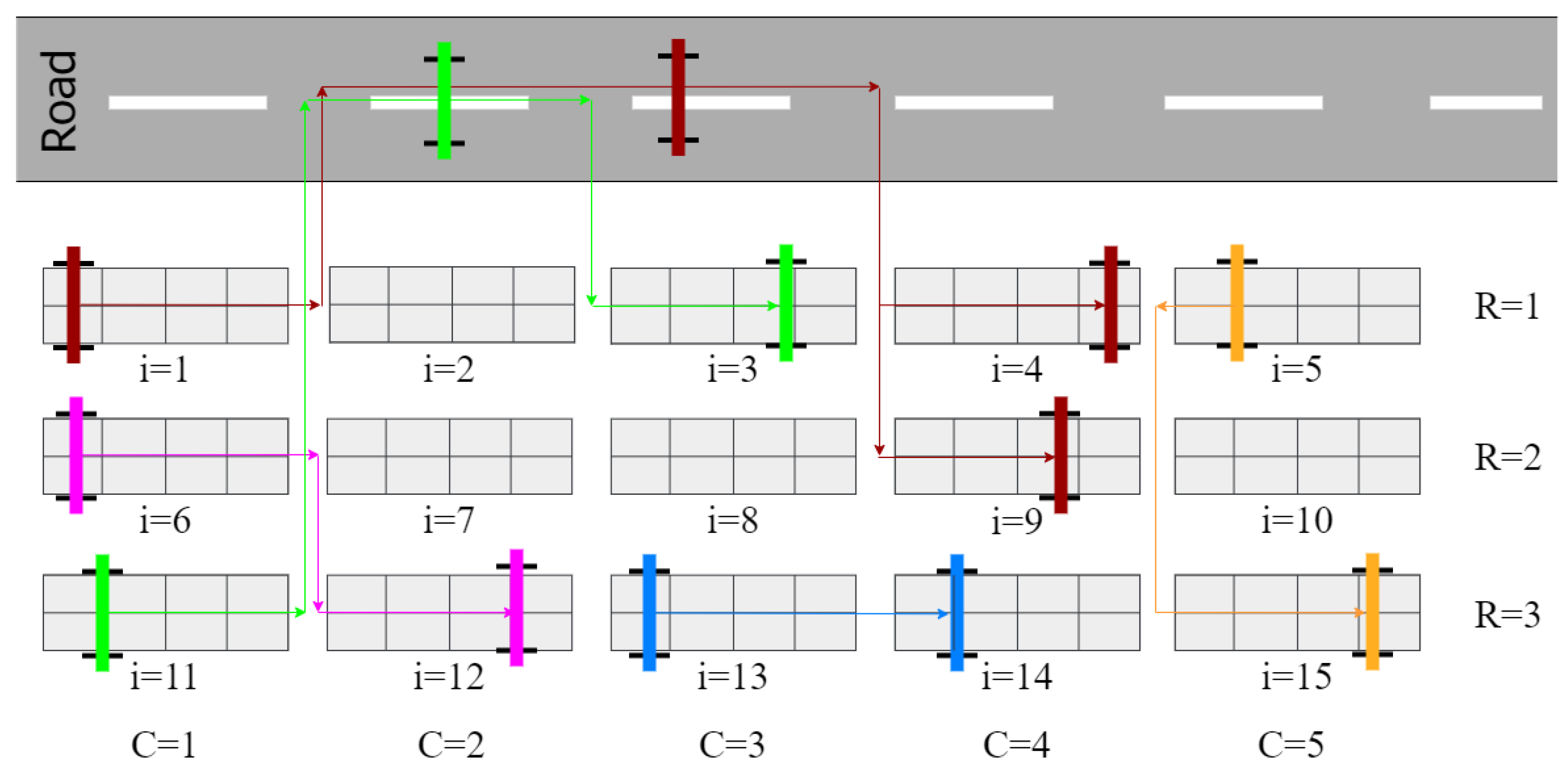
Figure 3 depicts an example of a yard area configuration and the possible YCs movements between the different YBs. The yard area is divided into five columns and three rows with 15 blocks ordered from (i = 1) to (i = 15). The sequence of movements depends on the position of the source and destination blocks and can be categorized into four groups: 1

• The two blocks are in the same row and adjacent columns (e.g., from i = 13 to i = 14). In this case, the traveling distance equals the horizontal distance between the two blocks.
• The two blocks are not in adjacent columns and any rows (e.g., from i = 1 to i = 4 or i = 9). In this case, the YC must travel to the road before proceeding to prevent any potential collisions with other yard cranes. The traveling distance equals the sum of the horizontal distance between the two blocks, the total vertical distance from the source and destination blocks to the road, and the distance required to rotate the crane tires by 90 degrees.
• The two blocks are in different rows and the same columns (e.g., from i = 5 to i = 15). The total traveling distance equals the vertical distance between the two YBs plus the distance required to rotate the crane tires by 90 degrees.
• The two blocks are in different rows and adjacent columns (e.g., i = 6 to i = 12). The traveling distance equals the sum of the horizontal and vertical distances between the two blocks and the distance required to rotate the crane tires by 90 degrees.

• Model assumptions

• Import and export containers are allocated to different storage locations.
• Each working day is divided into three shifts of 8 h, and each shift is divided into 8 TWs.
• All container data, such as container size, weight, vessel departure time, and hinterland destination, are known in advance.
• Each truck can be assigned to four containers at most (i.e., two export and two import containers), and the maximum weight each truck can accommodate is 30 tons.
• Due to safety concerns, a maximum number of two-yard cranes can exist in each YB during each shift.
• The number of YCs already existing at each YB in the first shift is known in advance, and all YCs have the same capacity.
• At any given time, the total number of yard cranes available at all YBs is always sufficient to handle the overall workload.

4. The Proposed Methodology

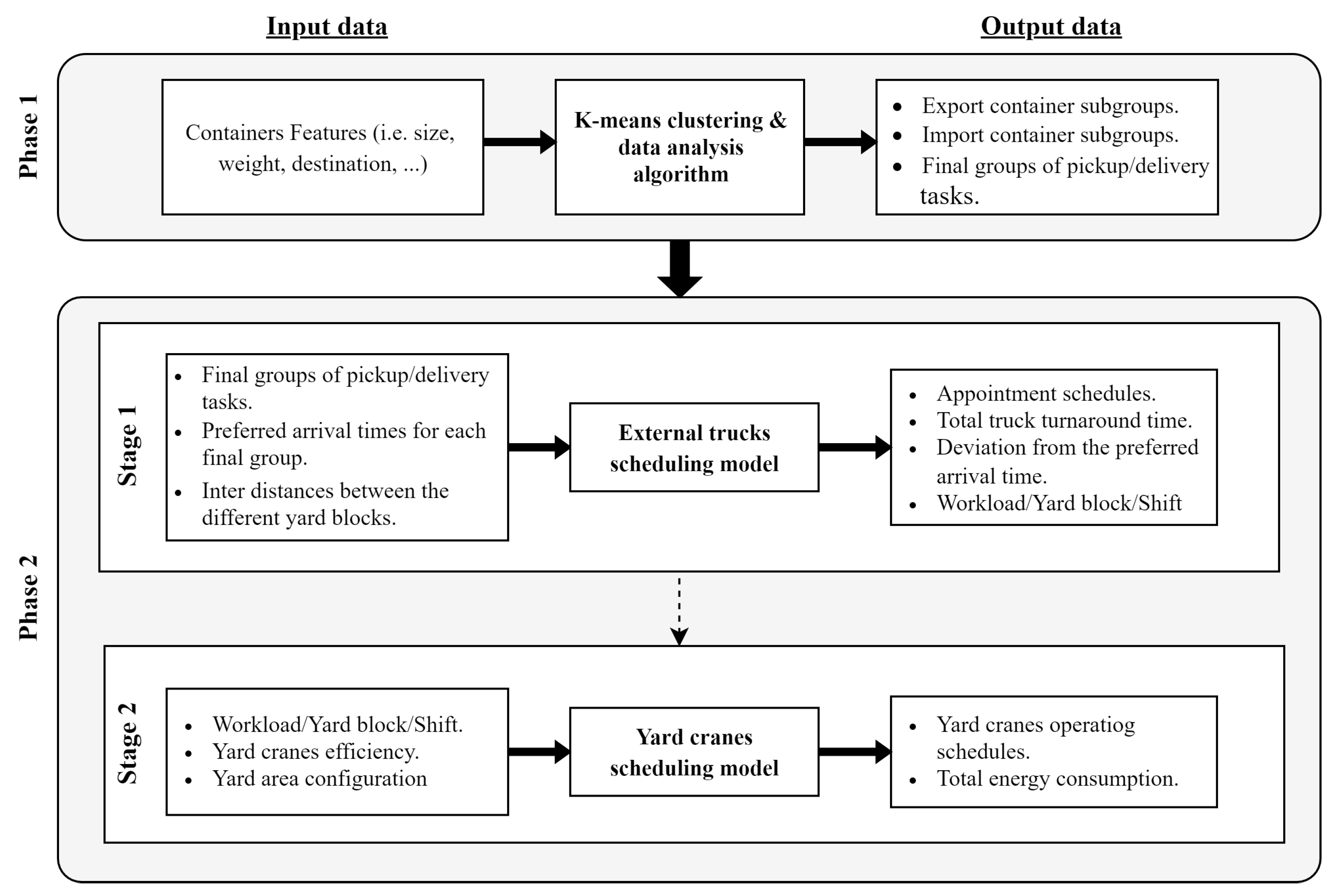
The adopted methodology in this study encompasses two distinct phases: data clustering and analysis, followed by two-stage mathematical optimization. Figure 4 defines the inputs and outputs for each phase.

The K-means clustering algorithm was chosen as the primary engine for phase 1 due to its straightforward implementation and capacity to elucidate the relationship between the number of clusters and the within-cluster squared error, providing valuable insights to the decision-maker, while mathematical modeling techniques are utilized in phase 2 to guarantee the attainment of an optimal solution to the problem.

4.1. Phase 1: Data Clustering and Analysis

Clustering is a dynamic approach for categorizing data into multiple sets based on the similarities among the features and attributes of data points [31]. In this phase, the daily container data are subjected to a series of clustering and analytical procedures to match export and import container trips aiming to minimize the total number of required trips to handle a set of containers and, consequently, the port-related emissions. Based on predefined criteria, two separate sets of subgroups are formed for export and import containers, which are denoted as (Ex1, Ex2) and (Im1, Im2), respectively. The resulting subgroups are then paired together to determine the minimum number of required trips to handle the sequence of tasks for each trip (i.e., Truck ID, (Ex1, Ex2), (Im1, Im2)).

According to Ezugwu et al. [32], the taxonomy of data clustering techniques can be divided into two main categories: (1) Partitioning methods involve dividing the data into distinct clusters based on predefined criteria. (2) Hierarchical methods involve creating a hierarchical structure of clusters by iteratively merging or splitting them.

In this work, a well-known partitioning clustering technique (K-means) is employed for several reasons, including its simplicity and efficiency in handling large datasets and its inherent capability to discern the patterns and structures within the data. Notably, a pivotal aspect that influenced our choice of the K-means clustering technique was its ability to determine the optimal number of clusters by minimizing the squared error within each cluster. The clustering process employed in this research incorporates a wide range of container features and characteristics. These features encompass both generic factors applicable to all containers, regardless of their type (import or export), as well as specific features pertaining exclusively to each type.

• General features

• Type: classifies each container as either an import or an export, denoting its respective cycle.
• Weight: indicates the weight of each individual container.
• Size: denotes the size of each container (i.e., 20 ft or 40 ft container).
• Collaboration: binary variable that signifies each trucking company’s disposition to share their trucks with other TCs.
• Distance: measures the inter-distance to be covered between the different yard blocks associated with each container handling task.

• Import containers features

• Delivery location: records the ultimate destination within the hinterland to which each import container is intended for delivery.
• Customs approval: binary variable that indicates whether the customs authority approved the clearance of each container or not. Compliance with this condition is essential for the container to be eligible for transportation from the terminal.
• Occupancy period: integer variable denotes the number of days each import container has spent waiting within the terminal premises. Containers with longer occupancy periods are given higher Priority.

• Export containers features

• Departure time: denotes the specific vessel departure time of each vessel associated with each export container.

4.2. Phase 2: Two-Stage Mathematical Optimization

In the second phase of the integrated approach, the mathematical optimization is executed in two stages. Firstly, a bi-objective optimization model is employed to assign the ETs to the designated TWs. Subsequently, a yard crane scheduling model is utilized to schedule the container handling operations with a particular emphasis on optimizing the moving energy consumption of the YCs.

4.2.1. External Truck Scheduling Model

The ETs appointment scheduling is carried out based on the mixed integer programming model originally devised by Caballini et al. [18]. The preferred arrival TW of each truck is determined by considering the earliest vessel departure time of the export containers within each final group. The final groups of pick-up/delivery tasks and their respective preferred arrival TW are executed through the bi-objective optimization model. The objective is to minimize the deviation between the appointed TW and the preferred arrival TW, while simultaneously minimizing the total turnaround time required to pick up/deliver all containers.

• Model sets and Parameters

• W: denotes the set of time windows (indexed by w).
• N: represents the resulting set of final groups to perform pickup/delivery tasks (indexed by n).
• I: the set of all terminal yard blocks (indexed by i).
• $I_n$: represents the sequential order of yard blocks visited by a truck associated with final group n, where $n\in N$.
• $u_n^i$: defines the number of export/import containers to be picked up or delivered in each final group $n\in N$ in and yard block $i\in I_n$.
• $g_n$: denotes the preferred arrival TW of each truck associated with final group $n\in N$.
• ${\alpha }_n$: signifies the priority assigned to each final group $n\in N$. The value of this parameter varies depending on whether it is a single cycle (${\alpha }_n=1$) or a double cycle (${\alpha }_n=2$).
• ${\delta }_{max}$: indicates the maximum allowable gap between the assigned TW and the TC’s preferred arrival TW for each truck.
• ${\beta }_w^i$: represents the congestion level of yard block $i\in I$ during each time window $w\in W$.
• ${\rho }_w^i$: denotes the productivity of the container handling resources at yard block $i\in I$ during time window $w\in W$.
• $Q_w^i$: identifies the number of available moves during time window $w\in W$ at yard block $i\in I$.
• $T_n^{IN}$: represents the time required for a truck associated with final group $n\in N$ to travel between the terminal gate and the yard block where the first container in the final group is stored.
• $T_n^{OUT}$: represents the required travel time for a truck associated with the final group $n\in N$ to reach the gate after completing the final pick up/delivery task in each final group.
• $T_n^{i,i+1}$: represents the required time for a truck associated with final group $n\in N$ to travel from yard block $i\in I_n$ to the subsequent yard block $a+1\in I_n$.

• Decision variables

• $x_{nw}=\left\{\begin{array}{cc}1,\hfill & \mathrm{if} \mathrm{final} \mathrm{group} n\in N \mathrm{is} \mathrm{assigned} \mathrm{to} \mathrm{time} \mathrm{window} w=1,\dots ,\mathrm{W}\hfill \\ 0,\hfill & \mathrm{otherwise}\hfill \end{array}\right.$
• ${\delta }_n$: integer variable represents the deviation between the appointed time window and the preferred arrival time of a truck associated with final group $n\in N$.
• $T{T}_{nw}$: continuous variable represents the turnaround time when a truck associated with final group $n\in N$ is assigned to a time window $w\in W$.

• Objective functions

$$Ob{j}_1:Min\sum _{n\in N}{\alpha }_n·{\delta }_n$$

(1)

$$Ob{j}_2:Min\sum _{n\in N}\sum _{w=1}^{W}T{T}_{nw}$$

(2)

• Constraints

$$\begin{array}{cccc}\hfill & \sum _{w=1}^W{x}_{nw}=1\hfill & \hfill & \forall n\in N\hfill \end{array}$$

(3)

$$\begin{array}{cccc}\hfill & \sum _{w=1}^{W}w·x_{nw}-g_n={\delta }_n\hfill & \hfill & \forall n\in N\hfill \end{array}$$

(4)

$$\begin{array}{cccc}\hfill & {\delta }_n\le {\delta }_{max}\hfill & \hfill & \forall n\in N\hfill \end{array}$$

(5)

$$\begin{array}{cccc}\hfill & \left(T_N^{in}+\sum _{i\in I_n}\left(\frac{u_n^i·60}{{\rho }_w^i·{\beta }_w^i}+T_n^{i,i+1}\right)+T_n^{out}\right)·x_{nw}\le T{T}_{nw}\hfill & \hfill & \forall n\in N,\forall w\in W\hfill \end{array}$$

(6)

$$\begin{array}{cccc}\hfill & \sum _{n\in N,i\in I_n}{u}_n^i·x_{nw}\le Q_w^i\hfill & \hfill & \forall n\in N,\forall w\in W\hfill \end{array}$$

(7)

$$\begin{array}{cccc}\hfill & x_{nw}\in (0,1)\hfill & \hfill & \forall n\in N,\forall w\in W\hfill \end{array}$$

(8)

$$\begin{array}{cccc}\hfill & {\delta }_n,T{T}_{nw}\ge 0\hfill & \hfill & \forall n\in N,\forall w\in W\hfill \end{array}$$

(9)

The two objective functions are described in Equations (1) and (2). The first objective (1) focused on reducing the gap between the TCs’ proposed arrival TW and the final appointments scheduled by CTs. The second objective (2) seeks to minimize the overall turnaround time for all trips required to handle the containers. Constraint (3) ensures that each final group of container tasks is served exclusively once, thereby preventing duplicate service occurrences. Constraint (4) calculates the gap between the TCs’ proposed arrival TW and the final appointment scheduled by CTs. Constraint (5) establishes the allowable upper limit for the gap between the TCs’ preferred arrival TW and the scheduled TW by terminal authorities (${\delta }_{max}$). This constraint ensures that the deviation between these two time parameters remains within an acceptable range. Constraint (6) calculates the turnaround time when a truck associated with the final group (n) is assigned to a time window (w). Due to the container handling the resource’s limited capacity, constraint (7) imposes limitations on the number of available moves that can be made at each yard block (i) during each time window (w). Constraint (8) and (9) delineates the domain of the decision variables of the model.

Various techniques exist in the literature to solve bi-objective optimization problems, such as (1) the weighted sum technique, in which the bi-objective optimization problem is converted into a single-objective problem by introducing weights to combine the objectives linearly, (2) goal programming, in which the goals are set for each objective, and the problem is formulated and solved as a multi-objective optimization with multiple constraints aiming to minimize the deviations from these goals, (3) evolutionary algorithms, which use mechanisms inspired by natural evolution to search for solutions in the objective space, such as genetic algorithms or particle swarm optimization, and (4) the epsilon constraint method, which transforms the bi-objective problem into a series of single-objective problems by adding constraints to one objective while optimizing the other. Different solutions on the Pareto front can be obtained by varying the constraint threshold.

Scheduling the external trucks’ arrivals at the terminal can be addressed from both stakeholders’ perspectives (CTs and TCs). The primary concern of CTs is to minimize the total turnaround time spent by all trucks. In contrast, satisfying the preferred arrival time without deviations is the main objective from the trucking companies’ perspective. Accordingly, it became imperative to explore a rational strategy that solves the proposed model considering both stakeholders’ perspectives and provides them with a solution that represents the trade-off between the total turnaround time and the gap between the TCs’ proposed arrival TW and the final appointments scheduled by CTs. Hence, the model was solved using the epsilon constraint method to obtain a Pareto front representation of the solution for the different turnaround time values and their corresponding gap values.

4.2.2. Yard Crane Scheduling Model

The traveled distance between source and destination blocks predominantly influences the moving energy consumption of YCs. Consequently, the efficient sequencing of YCs’ movements plays a crucial role in conserving energy. In this stage, the workload resulting from applying the ETs scheduling model is fed into an integer programming model to obtain the optimum schedules for YC operations that minimize the total moving energy consumption.

• Model sets and Parameters

• $RB$: represents the number of blocks in each row (indexed by R).
• $CB$: represents the number of blocks in each column (indexed by C).
• $TB$: represents the total number of blocks present in the yard area.
• $TS$: denotes the number of planning shifts in a decision-making cycle (i.e., daily shifts).
• $h_{it}$: defines the number of required yard cranes to satisfy the workload at block (i) at shift (t).
• $w_{it}$: the workload corresponding to yard block (i) during each shift (t).
• $b_{it}$: defines the number of yard cranes already existing at block (i) during shift (t).
• $D_{ij}$: represents the distance from source block (i) to destination block (j).
• $D_{cl}$: represents the horizontal distance a YC travels between every two consecutive columns.
• $D_{rw}$: represents the vertical distance a YC travels between every two consecutive rows.
• $D_R$: defines the vertical distance a YC travels between the first row (R = 1) and the road.
• $R_e$: represents the average efficiency of the yard cranes (RTGCs) in terms of TEU/minute.
• $t_c$: defines the time capacity of each yard crane during each shift in terms of minutes/shift.
• $e_c$: defines the average moving energy consumption of an RTGC in terms of Liter/meters.
• v: defines the velocity of the yard crane in terms of meters/min.
• $T_r$: represents the time required to rotate the yard crane tires by 90 degrees.
• S: represents the number of spare crane source locations
• $D_{sj}$: The yard crane traveling distance from a spare cranes’ location s to block j (in meters).

Based on the description of YC’s movements between the different yard blocks provided in Section 3.2, the distance ($D_{ij}$) from source block (i) to destination block (j) can be calculated as follows:

$$D_{(i,j)}=\left\{\begin{array}{cc}|C\left(i\right)-C\left(j\right)|·D_{cl};\hfill & \mathrm{if}R\left(i\right)=R\left(j\right),\left|C\right(i)-C(j\left)\right|=1\hfill \\ |R\left(i\right)-R\left(j\right)|·D_{rw}+2V·T_r;\hfill & \mathrm{if}R\left(i\right)\ne R\left(j\right),C\left(i\right)=C\left(j\right)\hfill \\ |C\left(i\right)-C\left(j\right)|+|R\left(i\right)-R\left(j\right)|+2V·T_r;\hfill & \mathrm{if}R\left(i\right)\ne R\left(j\right),\left|C\right(i)-C(j\left)\right|=1\hfill \\ 0;\hfill & \mathrm{if}i=j\hfill \\ |C\left(i\right)-C\left(j\right)|·D_{cl}+|R\left(i\right)-R\left(1\right)|·D_{rw}+|R\left(j\right)-R\left(1\right)|·D_{rw}+2D_R+4V·T_r;\hfill & \mathrm{otherwise}\hfill \end{array}\right.$$

The number of yard cranes ($h_{it}$) required to satisfy the workload ($w_{it}$) can be calculated from Equation (10) [29].

$$h_{it}=\frac{w_{it}}{{\mathrm{R}}_{\mathrm{e}}\times t_c}$$

(10)

Decision variables

• $F_{ijt}$: Number of yard cranes transferred from source block (i) to destination block (j) during shift (t).
• $P_{sjt}$: Number of spare cranes transferred from spare cranes source (s) to block (j) during shift (t).

Objective function

$$Minz=\sum _{t=1}^{TP}{E}_t$$

(11)

where $E_t$ represents the total moving energy consumption in all blocks during each shift (t).

$$\begin{array}{cccc}\hfill & E_t=\sum _{i=1}^{TB}\sum _{j=1}^{TB}{F}_{ijt}·D_{ij}·e_c+2·\sum _{s=1}^S\sum _{j=1}^{TB}{P}_{sjt}·D_{sj}·e_c\hfill & \hfill & \forall t\in TS\hfill \end{array}$$

(12)

Constraints

$$\begin{array}{cccc}\hfill & \sum _{j=1}^{TB}{F}_{ijt}\le 2\hfill & \hfill & \forall i\in TB,\forall t\in TS\hfill \end{array}$$

(13)

$$\begin{array}{cccc}\hfill & b_{jt}+\sum _{i=1}^{TB}{F}_{ijt}+\sum _{s=1}^S{P}_{sjt}\le 2\hfill & \hfill & \forall j\in TB,\forall t\in TS\hfill \end{array}$$

(14)

$$\begin{array}{cccc}\hfill & h_{jt}-b_{jt}\le \sum _{i=1}^{TB}{F}_{ijt}+\sum _{s=1}^S{P}_{sjt}\hfill & \hfill & \forall j\in TB,\forall t\in TS\hfill \end{array}$$

(15)

$$\begin{array}{cccc}\hfill & if{b}_{jt}\le h_{jt},then\sum _{i=1}^{TB}{F}_{jit}=0\hfill & \hfill & \forall j\in TB,\forall t\in TS\hfill \end{array}$$

(16)

$$\begin{array}{cccc}\hfill & b_{i(t+1)}=b_{it}-\sum _{j=1}^{TB}{F}_{ijt}+\sum _{j=1}^{TB}{F}_{jit}\hfill & \hfill & \forall i\in TB,\forall t\in TS\hfill \end{array}$$

(17)

$$\begin{array}{cc}\hfill & \sum _{s=1}^S\sum _{j=1}^{TB}\sum _{t=1}^{TS}{P}_{sjt}\le 3\hfill \end{array}$$

(18)

$$\begin{array}{cccc}\hfill & F_{ijt},P_{sjt}\in (0,1,2)\hfill & \hfill & \forall i,j\in TB,\forall t\in TS\hfill \end{array}$$

(19)

The objective function (11) seeks the minimization of the YC’s total moving energy consumption over all yard blocks during each shift. Equation (12) comprises the two constituent terms that collectively account for the energy consumption attributed to the crane’s movement between the different yard blocks. The first term represents the YCs energy consumption resulting from moving from each source block (i) to destination block (j), predominantly influenced by the distance traversed between these blocks. The second term represents the spare crane’s energy consumption when they move from their designated location to the destination block (j), and it is multiplied by two as each spare crane has to return to the spare crane location at the end of the day. Constraint (13) states that the number of YCs that can be moved from each source block (i) to all destination blocks during each shift cannot exceed two YCs. Due to safety concerns, constraint (14) ensures that the total number of YCs at each block during each shift is limited to two YCs. Constraint (15) ensures that the total number of YCs moving to each block (j) satisfies the number of YCs required to be delivered. Constraint (16) imposes a restriction on the relocation of yard cranes from any block. This restriction applies when the number of yard cranes available in a specific block is less than the number required to fulfill the workload assigned to that block during each shift. Constraint (17) updates the number of YCs already existing at each yard block at the beginning of each new shift (t + 1). Constraint (18) limits the available number of spare cranes. The domain of the two decision variables is defined in constraint (19).

5. Results and Analysis

In this section, a series of numerical experiments are conducted to investigate the performance of the proposed integrated approach. All experiments were conducted, and the results were analyzed on a computer equipped with an Intel i7-9750H CPU of 2.6 GHz and 16 GB of RAM. The implementation of the K-means clustering algorithm was performed in R programming language. The ETs scheduling model and the YCs scheduling model were coded in Python programming language and optimized using the Gurobi-Python optimization package.

A dataset comprising 2500 containers was generated and allocated across three eight-hour daily shifts. Specifically, 700 containers were assigned to the first shift (00:00–08:00), 1000 to the second (08:00–16:00), and 800 to the third shift (16:00–00:00). Among all containers, the percentage of import containers is 70%. A number of eight-yard blocks were considered; five were dedicated to import containers and three to export containers. The number of yard cranes available is eight. Moreover, 70% of all TCs agreed to collaborate by sharing the capacity of their trucks with each other. Considering the TCs’ satisfaction, a maximum tolerance of two time windows was set to the allowable deviations (${\delta }_{max}$) between the finally assigned and the TCs’ preferred arrival.

5.1. Results of Data Clustering and Analysis

The critical rationale for opting for the K-means clustering technique is its ability to provide the decision maker with crucial insights regarding the relationship between the number of clusters and the within-cluster squared error. This relationship is pivotal in determining an optimal number of clusters for the given dataset.

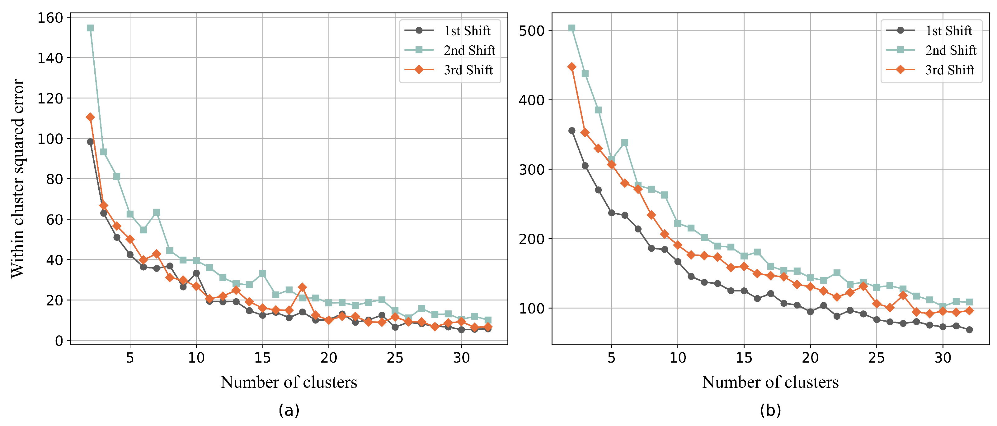
Figure 5 depicts the elbow plots of the three daily shifts for export and import containers. As an illustration, 25 clusters were chosen for the export containers, as further increasing the number of clusters was found to have a negligible impact on reducing the within-cluster squared error.

Based on the approvals of the customs authorities, only 1633 containers out of the 2500 containers were allowed to be picked up/delivered. In the base case operational scenario of a typical container terminal where trucks exclusively operate in single-cycle truck trips, it necessitated 1633 distinct truck trips to handle all containers. In contrast, a dual-cycle trip arrangement becomes feasible by adopting the proposed K-means clustering and data analysis approach. This progressive approach substantially diminishes the required number of truck trips to a significantly reduced count of 1057. This underscores the efficiency enhancements and operational optimizations achievable by implementing the proposed methodology.

The amount of ${\mathrm{CO}}_2$ emissions is directly proportional to the traveled distance through each trip and can be calculated based on Equation (20) [33].

$$\mathrm{Greenhouse}\mathrm{gas}\mathrm{emissions}=D\times W\times EF$$

(20)

where:

• D: represents the traveled distance (in miles).
• W: represents the weight of the shipment (in tons).
• EF: represents the ${\mathrm{CO}}_2$ emission factor (gram/ton-mile)

The outcomes derived from the base case operational scenario for the first, second, and third shifts are depicted in

Table 2. Base case scenario results of the first shift.

Trip ID	Ex Containers ID	Im Containers ID	Visited YBs	Distance (m)	CO2 Emissions (gram)
1	2	—	(7)	1290	3882.229
2	33	—	(7)	1290	3882.229
3	280	—	(6)	2180	6560.666
4	312	—	(7)	1290	3882.229
5	335	—	(7)	1290	3882.229
6	—	211	(3)	1236	3719.171
7	—	222	(1)	2000	6018.96
8	—	518	(4)	830	2497.868
9	—	530	(3)	1236	3719.171
—	—	—	—	—	—
455	—	544	(5)	1300	3912.324
∑				642,066	1,932,285

,

Table 3. Base case scenario results of the second shift.

Trip ID	Ex Containers ID	Im Containers ID	Visited YBs	Distance (m)	CO2 Emissions (gram)
1	87	—	(6)	2180	6560.66
2	127	—	(7)	1290	3882.229
3	138	—	(7)	1290	3882.229
4	151	—	(7)	1290	3882.229
5	153	—	(7)	1290	3882.229
6	—	635	(3)	1236	3719.171
7	—	642	(2)	1146	3448.864
8	—	681	(5)	1300	3912.324
9	—	814	(3)	1236	3719.717
—	—	—	—	—	—
658	—	844	(1)	2000	6018.96
∑				928,856	2,795,374

and

Table 4. Base case scenario results of the third shift.

Trip ID	Ex Containers ID	Im Containers ID	Visited YBs	Distance (m)	CO2 Emissions (gram)
1	628	—	(7)	1290	3882.229
2	40	—	(6)	2180	6560.666
3	117	—	(7)	1290	3882.229
4	201	—	(8)	1120	3370.618
5	230	—	(6)	2180	6560.666
6	—	599	(3)	1236	3719.717
7	—	639	(2)	1146	3448.864
8	—	688	(4)	830	2497.868
9	—	720	(4)	830	2497.868
—	—	—	—	—	—
520	—	764	(4)	830	2497.868
∑				734,436	2,210,270

, respectively. For instance, Table 3 delineates the aggregate distance covered and the consequent volume of ${\mathrm{CO}}_2$ emissions attributed to the 658 truck trips undertaken during the second shift, which only involved the transportation of a single container (i.e., empty trips).

In contrast, the proposed K-means clustering and data analysis phase results are depicted in

Table 5. The proposed K-means clustering and data analysis results of the first shift.

Trip ID	Ex Containers ID	Im Containers ID	Visited YBs	Distance (m)	CO2 Emissions (gram)
1	(2, 33)	(373, 391)	(7, 7, 3, 3)	1296	3900.286
2	(280, 312)	(408, 661)	(6, 7, 3, 3)	2089	6286.804
3	(335, 406)	(551, 565)	(7, 8, 4, 4)	1333	4011.637
4	(509, 533)	(18, 124)	(6, 7, 3, 3)	2089	6286.804
5	(559, 572)	(236, 394)	(6, 6, 1, 1)	2160	6500.477
6	(607, 61)	(353, 558)	(8, 7, 2, 3)	1746	5254.552
7	(26, 81)	(60, 260)	(8, 6, 1, 2)	2201	6623.865
8	(92, 117)	(246, 438)	(7, 8, 4, 2)	1546	4652.656
9	(193, 200)	(416, 511)	(7, 6, 1, 5)	2083	6268.747
—	—	—	—	—	—
287	—	544	(5)	1300	3912.324
∑				429,084	1,291,320

,

Table 6. The proposed K-means clustering and data analysis results of the second shift.

Trip ID	Ex Containers ID	Im Containers ID	Visited YBs	Distance (m)	CO2 Emissions (gram)
1	(638, 838)	(95, 715)	(8, 7, 3, 3)	1451	4366.755
2	(82, 190)	(521, 562)	(6, 7, 3, 3)	2089	6286.804
3	(219, 221)	(300, 625)	(6, 7, 3, 3)	2089	6286.804
4	(228, 267)	(53, 565)	(6, 7, 3, 3)	2089	6286.804
5	(302, 359)	(49, 941)	(7, 6, 1, 1)	2063	6208.557
6	(373, 433)	(235, 760)	(7, 8, 4, 4)	1333	4011.637
7	(526, 529)	(366, 464)	(8, 6, 1, 1)	2238	6735.216
8	(611, 673)	(738, 939)	(6, 7, 3, 3)	2089	6286.804
9	(683, 687)	(131, 198)	(8, 6, 1, 1)	2238	6735.216
—	—	—	—	—	—
422	—	969	(4)	830	2497.868
∑				641,328	1,930,064

and

Table 7. The proposed K-means clustering and data analysis results of the third shift.

Trip ID	Ex Containers ID	Im Containers ID	Visited YBs	Distance (m)	CO2 Emissions (gram)
1	(83, 352)	(371, 486)	(6, 8, 4, 4)	2146	6458.344
2	(332, 462)	(130, 175)	(6, 6, 1, 1)	2160	6500.477
3	(139, 210)	(109, 723)	(7, 7, 3, 3)	1296	3900.286
4	(261, 299)	(62, 358)	(8, 8, 4, 4)	1008	3033.556
5	(401, 404)	(75, 433)	(8, 7, 3, 3)	1451	4366.755
6	(437, 457)	(444, 538)	(8, 6, 3, 1)	2871	8640.217
7	(676, 754)	(516, 595)	(8, 6, 2, 1)	2860	8607.113
8	(25, 113)	(68, 626)	(7, 8, 4, 4)	1333	4011.637
9	(83, 352)	(371, 486)	(6, 8, 4, 4)	2146	6458.344
—	—	—	—	—	—
348	—	764	(4)	830	2497.868
∑				516,464	1,554,288

. As an illustration, Table 6 exhibits that by performing dual-cycle truck trips, the number of required truck trips during the second shift was effectively reduced from 658 to 422, leading to a remarkable reduction of approximately 36% in the number of empty truck trips. Compared to the base case operational scenario, this strategy yielded a substantial decrease of approximately 866 kg in the overall ${\mathrm{CO}}_2$ emissions, demonstrating a notable advancement in environmental sustainability.

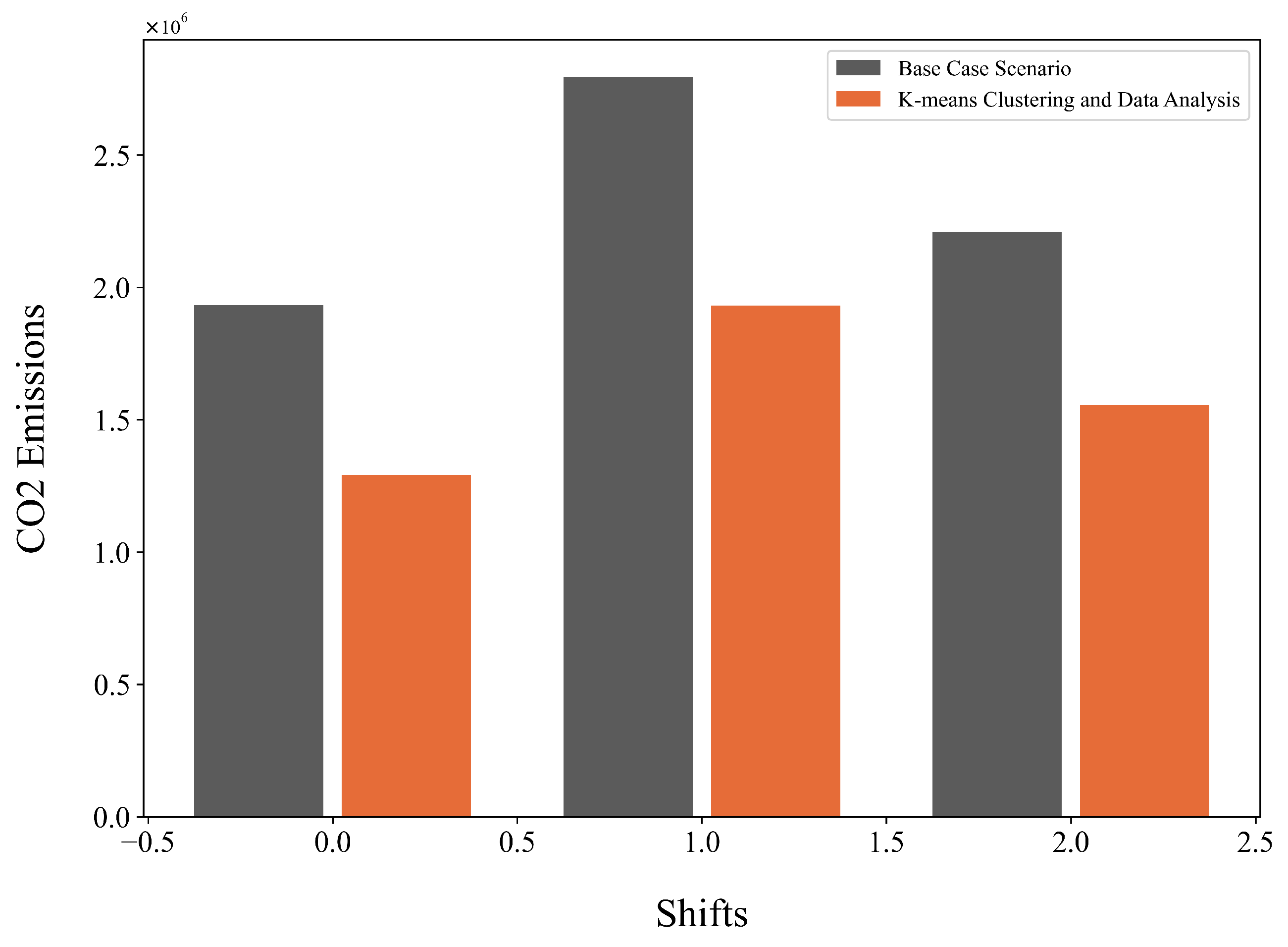
Figure 6 encapsulates a concise overview of the application of the proposed K-means clustering and data analysis approach compared to the base case operational scenario in the context of CO₂ emissions amount over the three daily shifts. The findings notably highlight that implementing the proposed approach substantially reduced port-related CO₂ emissions across all shifts by about 31.2%.

5.2. Results of the External Truck Scheduling Model

The container pick-up and delivery processes involve the collaboration of two primary stakeholders: the terminal operators and the trucking companies. To develop an effective TAS that promotes adherence from both parties, it becomes essential to account for the two parties’ distinct objectives and concerns. The proposed ETs scheduling model is designed with a dual objective in mind, aiming to minimize the total turnaround time (a central concern for CTs) and satisfy the preferred arrival times of the TCs (TCs’ main objective). To reconcile the potential trade-offs between these two objectives, the epsilon constraint method was employed to solve the model. The results of the ETs scheduling model are comprehensively presented in

Table 8. External truck scheduling model results for the first shift.

				TCs’ Perspective			CTs’ Perspective
Trip ID	Ex Containers ID	Im Containers ID	Preferred TW (g)	Assigned TW	Deviation ($\mathbf{\delta }$)	TT (min)	Assigned TW	Deviation ($\mathbf{\delta }$)	TT (min)
1	(2, 33)	(373, 391)	3	4	1	167.4659	4	1	167.4659
2	(280, 312)	(408, 661)	2	2	0	155.9099	2	0	155.9099
3	(335, 406)	(551, 565)	3	3	0	143.495	3	0	143.495
4	(509, 533)	(18, 124)	3	3	0	146.8062	3	0	146.806
5	(559, 572)	(236, 394)	2	2	0	777.4759	4	2	206.529
6	(607, 610)	(353, 558)	3	3	0	121.7324	4	1	96.637
7	(26, 81)	(60, 260)	7	7	0	207.0235	8	1	230.536
8	(92, 117)	(246, 438)	7	7	0	305.9717	8	1	145.803
9	(193, 200)	(416, 511)	7	7	0	109.6993	7	0	109.699
—	—	—	—	—	—	—	—	—	—
287	—	544	8	8	0	90.6933	6	2	63.354
∑					7	20,256.36		156	16,238.82

,

Table 9. External truck scheduling model results for the second shift.

				TCs’ Perspective			CTs’ Perspective
Trip ID	Ex Containers ID	Im Containers ID	Preferred TW (g)	Assigned TW	Deviation ($\mathbf{\delta }$)	TT (min)	Assigned TW	Deviation ($\mathbf{\delta }$)	TT (min)
1	(638, 838)	(95, 715)	3	3	0	86.49794	3	0	86.49794
2	(82, 190)	(521, 562)	1	1	0	158.901	3	2	111.8636
3	(219, 221)	(300, 625)	1	1	0	158.901	3	2	111.8636
4	(228, 267)	(53, 565)	1	1	0	158.901	3	2	111.8636
5	(302, 359)	(49, 941)	1	1	0	361.5819	3	2	153.1081
6	(373, 433)	(235, 760)	1	1	0	236.4828	2	1	164.0493
7	(526, 529)	(366, 464)	2	2	0	192.3909	3	1	159.7989
8	(611, 673)	(738, 939)	2	2	0	237.7281	3	1	111.8636
9	(683, 687)	(131, 198)	3	3	0	86.49794	3	2	159.7989
—	—	—	—	—	—	—	—	—	—
422	—	696	4	4	0	90.693	6	2	18.022
∑					3	27,526.56		318	20,799.93

and

Table 10. External truck scheduling model results for the third shift.

				TCs’ Perspective			CTs’ Perspective
Trip ID	Ex Containers ID	Im Containers ID	Preferred TW (g)	Assigned TW	Deviation ($\mathbf{\delta }$)	TT (min)	Assigned TW	Deviation ($\mathbf{\delta }$)	TT (min)
1	(83, 352)	(371, 486)	5	5	0	174.4335	6	1	114.4917
2	(332, 462)	(130, 175)	4	4	0	380.8955	6	2	138.1819
3	(139, 210)	(109, 723)	3	3	0	237.1177	4	1	146.404
4	(261, 299)	(62, 358)	3	3	0	128.3456	3	0	128.3456
5	(401, 404)	(75, 433)	2	2	0	196.0527	4	2	122.4761
6	(437, 457)	(444, 538)	1	1	0	181.7152	3	2	129.6602
7	(676, 754)	(516, 595)	2	2	0	154.5623	2	0	154.5623
8	(25, 113)	(68, 626)	6	6	0	136.562	6	0	136.562
9	(119, 160)	(283, 560)	6	6	0	98.23624	6	0	98.23624
—	—	—	—	—	—	—	—	—	—
348	—	764	4	4	0	37.766	6	2	18.49252
∑					0	18,920.69		233	15,317.41

across the three operational shifts.

The first column contains the identification number of each truck trip, while the second and third columns hold the number of export and import containers corresponding to each trip, respectively. Additionally, the fourth column identifies the preferred arrival time of each truck. The solution from the perspective of TCs is depicted in columns 5, 6, and 7, and column 5 carries the final appointed time window for each truck trip. Column 6 shows the gap between the TCs’ preferred arrival time window and the final appointment, whereas column 7 holds the corresponding turnaround time for each trip. Similarly, columns 8, 9, and 10 display the solution from the standpoint of CTs.

As an illustration, Table 9 encompasses a comprehensive overview of the solutions achieved during the second shift, considering the viewpoints of both TCs and CTs. From the trucking companies’ standpoint, the primary concern is satisfying the desired arrival TW, so in most cases, the solution of the proposed model was able to meet the TCs’ preferred arrival TW. In contrast, the terminal operators are more concerned with minimizing the total turnaround time, sometimes necessitating reallocating the TCs’ preferred arrival TWs. For instance, in the second trip (Trip ID = 2), the desired arrival time is the first TW. Adhering to this desired TW would result in a turnaround time of approximately 159 min. However, deviating by two TWs would reduce the turnaround time by about 47 min.

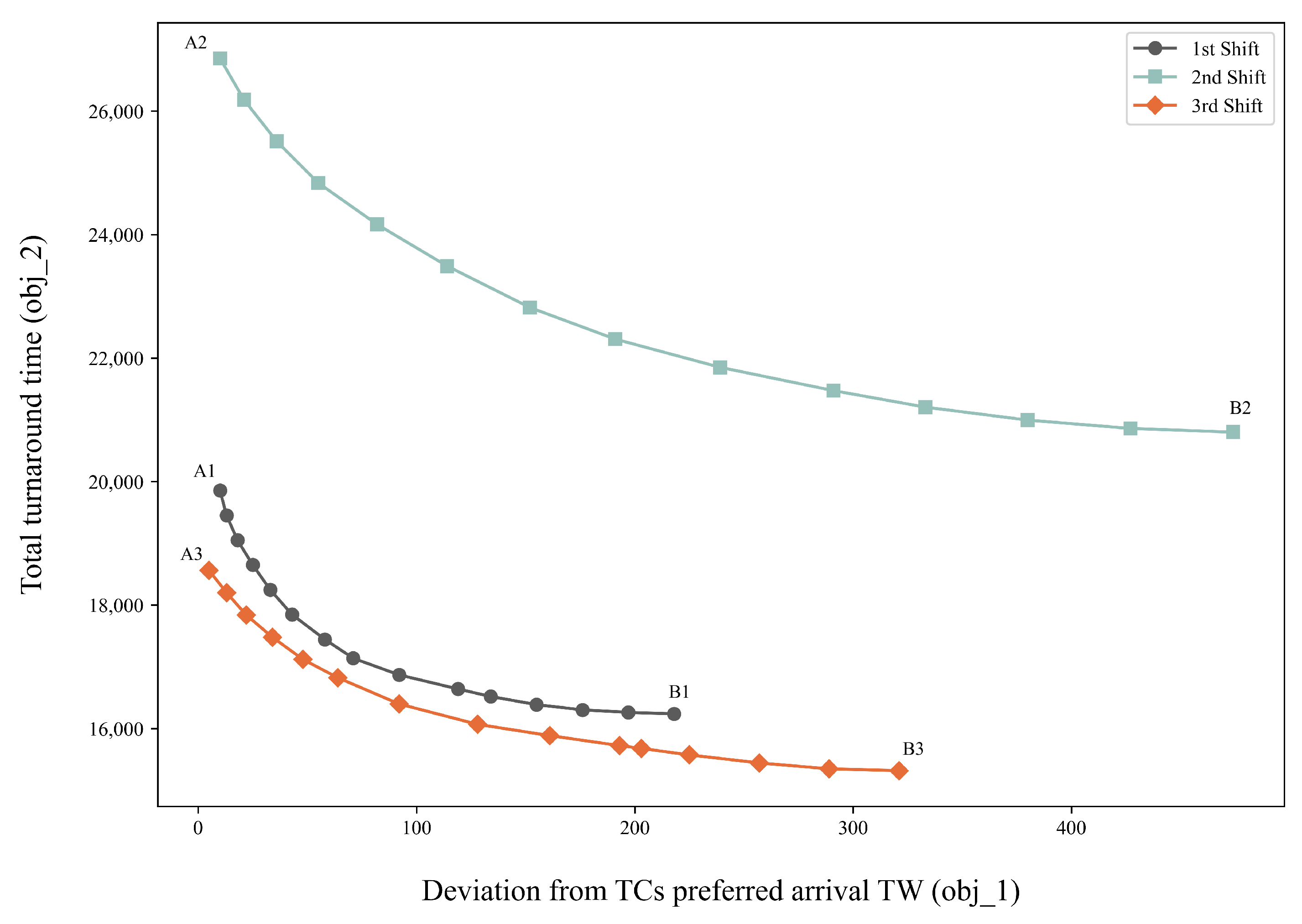
Figure 7 illustrates the Pareto-front solutions for the three daily shifts. Points A1, A2, and A3 correspond to solutions viewed from the perspective of trucking companies, emphasizing minimal gaps between the assigned TW and their preferred arrival TW. Conversely, points B1, B2, and B3 depict solutions from the standpoint of terminal operators, prioritizing minimal total turnaround time.

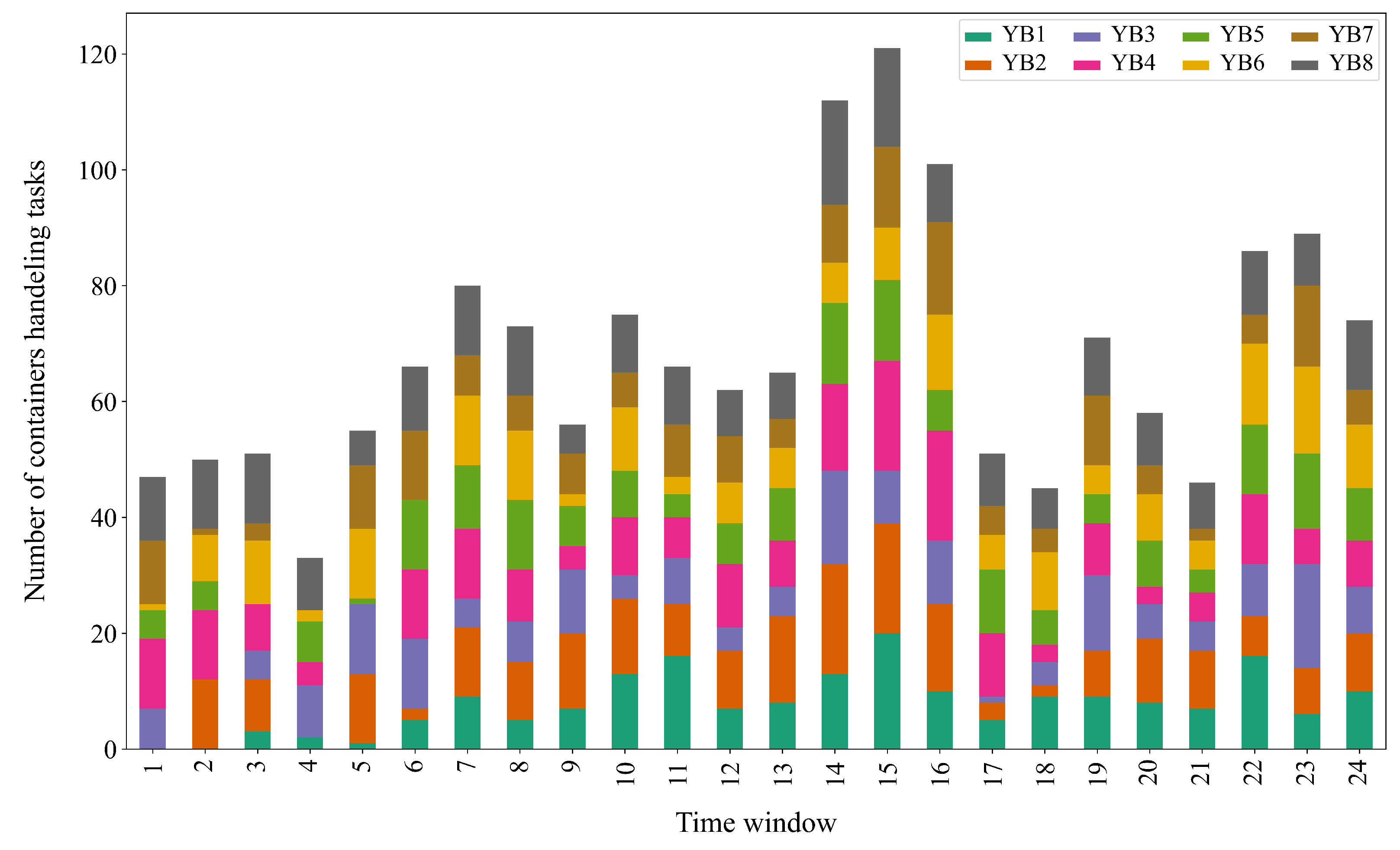
Figure 8 displays the pickup/delivery workload distribution across the different yard blocks for each designated time window from the perspective of the CT. The most significant portion of appointments was observed during the second shift. This observation can be attributed to the alignment of the second shift with the peak activity hours typically observed in numerous terminals.

5.3. Results of Yard Crane Scheduling Model

After finalizing the external trucks’ appointment schedules, the workload attributed to each yard block within every shift becomes ascertainable. Subsequently, the YC scheduling model minimizes the total energy consumption incurred by YC movements between the different YBs to accommodate these workloads.

The quantity of available cranes remains constant, undergoing alteration solely upon the terminal authority’s decision to augment the yard crane fleet’s scale. At the beginning of the first shift, the available number of YCs is randomly distributed over all the blocks.

Table 11. Results of yard cranes scheduling model.

First Shift (00:00–08:00)
Block ID	1	2	3	4	5	6	7	8	Total number of YCs	Total distance (m)	Energy consumption (L)
Workload ($w_{it}$)	47	50	51	33	55	66	80	73
Available RTGCs ($b_{it}$)	0	2	1	0	1	0	1	2	7
Required RTGCs ($h_{it}$)	1	1	1	1	1	1	1	1	8
RTGCs Movement ($F_{ijt}$)	from 2	to 1		from 8				to 4	2	1456	69.12
Spare cranes ($P_{sjt}$)						from s			1	1000
Second Shift (08:00–16:00)
Workload ($w_{it}$)	56	75	66	62	65	112	121	101
Available RTGCs ($b_{it}$)	1	1	1	1	1	1	1	1	8
Required RTGCs ($h_{it}$)	1	1	1	1	1	2	2	1	10
RTGCs Movement ($F_{ijt}$)											80
Spare cranes ($P_{sjt}$)						from s	from s		2	2000
Third Shift (16:00–00:00)
Workload ($w_{it}$)	51	45	71	58	46	86	89	74
Available RTGCs ($b_{it}$)	1	1	1	1	1	2	2	1	10
Required RTGCs ($h_{it}$)	1	1	1	1	1	1	1	1	8
RTGCs Movement ($F_{ijt}$)
Spare cranes ($P_{sjt}$)
∑										4456	149.12

encapsulates the outcomes engendered by the yard crane scheduling model, elucidating the allocation of YCs among the assorted blocks within the container yard. The tabulation gives insights into the count of available yard cranes at the commencement of each shift, the requisite YCs needed to fulfill the workload, and the crane movements originating from and destined for each block. The cumulative traveling distance between blocks and the corresponding energy consumption is also meticulously delineated. For instance, during the first shift, the extant count of YCs present at yard blocks 1, 4, and 6 proves insufficient for the workload. Conversely, at blocks 2 and 8, the pre-existing number of YCs surpasses the stipulated requirement. Consequently, one YC is relocated from yard block 2 to block 1, and another is transposed from block 8 to block 4. Similarly, a spare crane is transferred to meet the workload at block 6, as no surplus YCs are available for reassignment from other blocks.

6. Conclusions and Future Directions

This article introduced a novel approach that synergizes data analysis and operations research by integrating data clustering and two-stage mathematical optimization to effectively mitigate ${\mathrm{CO}}_2$ emissions associated with port activities. The proposed approach is centered on increasing the number of dual-cycle truck trips, thereby minimizing the number of truck trips required for container pickup and delivery tasks. This approach encompasses two principal phases: the K-means clustering and data analysis phase and a two-stage mathematical model tailored for scheduling external trucks and yard cranes.

The K-means clustering and data analysis phase is geared towards curbing the ecological impact of port operations by minimizing the frequency of empty truck trips. Furthermore, the external truck scheduling model pursues dual objectives: (1) truncating the cumulative turnaround duration for all truck trips, and (2) increasing the trucking companies’ satisfaction by minimizing the gap between their preferred arrival time windows and the final appointments. In addition, the YC scheduling model aims to minimize the total moving energy consumption of YCs by optimizing their movement between different yard blocks to meet the workload requirements.

The obtained outcomes demonstrated the efficacy of this approach, showcasing a noteworthy reduction in daily ${\mathrm{CO}}_2$ emissions by approximately 31%. Additionally, the proposed approach provided a pivotal trade-off to terminal operators and trucking companies between reallocating preferred truck arrival time windows and optimizing turnaround times for each trip.

Finally, the findings of this article present a compelling incentive for both stakeholders in container terminals and trucking companies to collaborate towards sustainable practices.

This study lays the groundwork for future sustainable container terminal operations research endeavors. However, it is essential to acknowledge the limitations of this work, specifically the focus solely on external trucks and yard cranes’ operations without accounting for other resources’ operations, such as quay cranes and berthing plans. In addition, this study assumes that all containers are stacked at the top of the block and it does not address container handling time in the yard area.

Hence, future research endeavors could address these limitations by investigating the potential benefits and implications of joining the external trucks and yard cranes scheduling models into one mathematical model to consider both aspects concurrently rather than implementing them as separate models. The integrated scheduling of ETs and YCs could also be extended to include the quay cranes assignment plan. Additionally, various sources of uncertainties could be considered to improve the simulation’s fidelity to real-world scenarios.

References

- United Nations Conference on Trade and Development (UNCTAD). Review of Maritime Transport 2022. Available online: https://unctad.org/rmt2022 (accessed on 22 June 2023).
- Lu, Q.; Yang, X.; Wang, R. Multi-Depot Vehicle Scheduling Optimization for Port Container Drop and Pull Transport. J. Coast. Res. 2019, 98, 325–329. [Google Scholar] [CrossRef]
- Torkjazi, M.; Huynh, N.N. Design of a Truck Appointment System Considering Drayage Scheduling and Stochastic Turn Time. Transp. Res. Rec. 2021, 2675, 342–354. [Google Scholar] [CrossRef]
- Im, H.; Yu, J.; Lee, C. Truck appointment system for cooperation between the transport companies and the terminal operator at container terminals. Appl. Sci. 2020, 11, 168. [Google Scholar] [CrossRef]
- Torkjazi, M.; Huynh, N.; Shiri, S. Truck appointment systems considering impact to drayage truck tours. Transp. Res. Part E Logist. Transp. Rev. 2018, 116, 208–228. [Google Scholar] [CrossRef]
- Jin, Z.; Lin, X.; Zang, L.; Liu, W.; Xiao, X. Lane allocation optimization in container seaport gate system considering carbon emissions. Sustainability 2021, 13, 3628. [Google Scholar] [CrossRef]
- Fan, H.; Ren, X.; Guo, Z.; Li, Y. Truck scheduling problem considering carbon emissions under truck appointment system. Sustainability 2019, 11, 6256. [Google Scholar] [CrossRef]
- Xu, B.; Liu, X.; Yang, Y.; Li, J.; Postolache, O. Optimization for a multi-constraint truck appointment system considering morning and evening peak congestion. Sustainability 2021, 13, 1181. [Google Scholar] [CrossRef]
- Wasesa, M.; Ramadhan, F.I.; Nita, A.; Belgiawan, P.F.; Mayangsari, L. Impact of overbooking reservation mechanism on container terminal’s operational performance and greenhouse gas emissions. Asian J. Shipp. Logist. 2021, 37, 140–148. [Google Scholar] [CrossRef]
- Lange, A.K.; Branding, F.; Schwenzow, T.; Zlotos, C.; Schwientek, A.K.; Jahn, C. Dispatching strategies of drayage trucks at seaport container terminals with truck appointment system. In Dynamics in Logistics, Proceedings of the 6th International Conference LDIC 2018, Bremen, Germany, 20–22 February 2018; Springer: Cham, Switzerland, 2018; pp. 162–166. [Google Scholar]
- Li, N.; Chen, G.; Govindan, K.; Jin, Z. Disruption management for truck appointment system at a container terminal: A green initiative. Transp. Res. Part D Transp. Environ. 2018, 61, 261–273. [Google Scholar] [CrossRef]
- Shao, Q.; Huang, M.; Zhang, S.; Zhang, Y. Simulation of truck arrivals at container terminal based on the interactive truck appointment system. Int. J. Shipp. Transp. Logist. 2022, 14, 141–171. [Google Scholar] [CrossRef]
- Azab, A.; Karam, A.; Eltawil, A. A simulation-based optimization approach for external trucks appointment scheduling in container terminals. Int. J. Model. Simul. 2020, 40, 321–338. [Google Scholar] [CrossRef]
- Ramírez-Nafarrate, A.; González-Ramírez, R.G.; Smith, N.R.; Guerra-Olivares, R.; Voß, S. Impact on yard efficiency of a truck appointment system for a port terminal. Ann. Oper. Res. 2017, 258, 195–216. [Google Scholar] [CrossRef]
- Zhang, X.; Zeng, Q.; Yang, Z. Optimization of truck appointments in container terminals. Marit. Econ. Logist. 2019, 21, 125–145. [Google Scholar] [CrossRef]
- Minh, C.C.; Noi, N.V. Optimising truck arrival management and number of service gates at container terminals. Marit. Bus. Rev. 2023, 8, 18–31. [Google Scholar] [CrossRef]
- Schulte, F.; Lalla-Ruiz, E.; González-Ramírez, R.G.; Voß, S. Reducing port-related empty truck emissions: A mathematical approach for truck appointments with collaboration. Transp. Res. Part E Logist. Transp. Rev. 2017, 105, 195–212. [Google Scholar] [CrossRef]
- Caballini, C.; Gracia, M.D.; Mar-Ortiz, J.; Sacone, S. A combined data mining–optimization approach to manage trucks operations in container terminals with the use of a TAS: Application to an Italian and a Mexican port. Transp. Res. Part E Logist. Transp. Rev. 2020, 142, 102054. [Google Scholar] [CrossRef]
- Chen, S.; Zeng, Q. Carbon-efficient scheduling problem of electric rubber-tired gantry cranes in a container terminal. Eng. Optim. 2022, 54, 2034–2052. [Google Scholar] [CrossRef]
- Zheng, F.; Man, X.; Chu, F.; Liu, M.; Chu, C. A two-stage stochastic programming for single yard crane scheduling with uncertain release times of retrieval tasks. Int. J. Prod. Res. 2019, 57, 4132–4147. [Google Scholar] [CrossRef]
- Li, J.; Yang, J.; Xu, B.; Yin, W.; Yang, Y.; Wu, J.; Zhou, Y.; Shen, Y. A Flexible Scheduling for Twin Yard Cranes at Container Terminals Considering Dynamic Cut-Off Time. J. Mar. Sci. Eng. 2022, 10, 675. [Google Scholar] [CrossRef]
- Mar-Ortiz, J.; Castillo-García, N.; Gracia, M.D. A decision support system for a capacity management problem at a container terminal. Int. J. Prod. Econ. 2020, 222, 107502. [Google Scholar] [CrossRef]
- Yu, K.; Yang, J. MILP model and a rolling horizon algorithm for crane scheduling in a hybrid storage container terminal. Math. Probl. Eng. 2019, 2019, 4739376. [Google Scholar] [CrossRef]
- Liu, W.; Zhu, X.; Wang, L.; Yan, B.; Zhang, X. Optimization Approach for Yard Crane Scheduling Problem with Uncertain Parameters in Container Terminals. J. Adv. Transp. 2021, 2021, 5537114. [Google Scholar] [CrossRef]
- He, J.; Tan, C.; Zhang, Y. Yard crane scheduling problem in a container terminal considering risk caused by uncertainty. Adv. Eng. Inform. 2019, 39, 14–24. [Google Scholar] [CrossRef]
- Galle, V.; Barnhart, C.; Jaillet, P. Yard crane scheduling for container storage, retrieval, and relocation. Eur. J. Oper. Res. 2018, 271, 288–316. [Google Scholar] [CrossRef]
- Zheng, F.; Man, X.; Chu, F.; Liu, M.; Chu, C. Two yard crane scheduling with dynamic processing time and interference. IEEE Trans. Intell. Transp. Syst. 2018, 19, 3775–3784. [Google Scholar] [CrossRef]
- Huang, S.Y.; Li, Y. Yard crane scheduling to minimize total weighted vessel loading time in container terminals. Flex. Serv. Manuf. J. 2017, 29, 689–720. [Google Scholar] [CrossRef]
- Sha, M.; Zhang, T.; Lan, Y.; Zhou, X.; Qin, T.; Yu, D.; Chen, K. Scheduling optimization of yard cranes with minimal energy consumption at container terminals. Comput. Ind. Eng. 2017, 113, 704–713. [Google Scholar] [CrossRef]
- Abdelmagid, A.M.; Gheith, M.S.; Eltawil, A.B. A comprehensive review of the truck appointment scheduling models and directions for future research. Transp. Rev. 2022, 42, 102–126. [Google Scholar] [CrossRef]
- Jain, A.K. Data clustering: 50 years beyond K-means. Pattern Recognit. Lett. 2010, 31, 651–666. [Google Scholar] [CrossRef]
- Ezugwu, A.E.; Ikotun, A.M.; Oyelade, O.O.; Abualigah, L.; Agushaka, J.O.; Eke, C.I.; Akinyelu, A.A. A comprehensive survey of clustering algorithms: State-of-the-art machine learning applications, taxonomy, challenges, and future research prospects. Eng. Appl. Artif. Intell. 2022, 110, 104743. [Google Scholar] [CrossRef]
- Mathers, J.; Wolfe, C.; Norsworthy, M.; Craft, E. The Green Freight Handbook; Environmental Defense Fund: Washington, DC, USA, 2014; Volume 86. [Google Scholar]
Figure 1.
emissions resulted from the World Fleet [
1].
Figure 2.
Illustrative scheme for single and dual-cycle truck trips.
Figure 3.
Yard area configuration and yard crane possible movements.
Figure 4.
The methodological framework of the proposed approach.
Figure 5.
Elbow plots resulted from K-means clustering during the three shifts for export containers (a) and for import containers (b).
Figure 6.
The amount of emissions resulted from the base case scenario VS the proposed data clustering and analysis approach.
Figure 7.
Pareto front representation for the daily shifts.
Figure 8.
Workload distribution over each YB during each Tw form CTs perspective.