
Optimizing Utilization of Transport Capacities in the Cold Chain by Introducing Dynamic Allocation of Semi-Trailers


Abstract
:1. Introduction
2. Literature Review
- Transport cost, is considered as one of the criteria in papers [1,2,3,4,5,6,7,8,9,10,11,12,13,14,15,16,17,18,19,20,21,22,23,24,25,26,27,28,29,30,31,32,33,34,35,36,37,38,39,40,41,42,43,44,45,46,47,48,49,50,51,52,53,54,55,56,57,58,59,60,61,62,63,64,65], and as a single optimization criterion in papers [46,47,48,49,50,51,52,53,54,55,56,57,58,59,60,61,62,63,64,65]. Optimizing transportation routes with the goal of minimizing costs involves defining the most efficient route that vehicles can take to reduce the variable costs (such as fuel, tolls, etc.) and fixed costs (such as vehicle workday costs, salaries of the drivers, maintenance, etc.), while complying with the planned itinerary. The shortest or the fastest route is not necessarily the most cost effective. The goal is to find the best combination of transport orders, in-the-route movements and travel time that would result in a reduction of total transport costs.
- Quality and safety are not considered as a single optimization criterion in any of the papers but are present as one of the criteria in papers [1,2,3,4,5,6,7,8,9,10,11,12,13,14,15,16,17,18,19,20,21,66,67,68,69,70,71,72]. Optimizing transport routes with the aim of meeting the quality standards such as ISO9001, HACCP (hazard analysis critical control point), GDP Pharma (good distribution practice) and safety of the substrate is about finding the best way to deliver the product with minimal risk of contamination or damage. Consolidating different kinds of products that can be transported without cross-contamination would result in better utilization of the transport capacities, which is in line with this criterion.
- Environmental impact is not considered as a single optimization criterion in any of the papers but is present as one of the criteria in papers [1,2,3,4,5,6,7,8,9,22,23,24,25,26,27,28,29,30,31,32,33,34,35,36,37,38,39,40,41,66,73,74,75,76]. Greenhouse gasses such as carbon dioxide, methane, and nitrous oxide are responsible for the warming of the Earth’s atmosphere, leading to climate change. Climate change affects our environment, lifestyle, and food production. Optimizing vehicle routes with the goal of protecting the environment is about finding the best route for vehicles to travel that would reduce harmful gas emissions, fuel consumption, and environmental impact.
- Customer satisfaction, as a single optimization criterion is present in paper [77], and as one of the criteria in papers [1,22,23,24,25,26,27,28,29,42,43,44,45,73]. Route optimization for customer satisfaction is about defining an itinerary that would enable timeliness in pick-up and delivery, minimizing delays, and the problems thereof. Consequently, the products are delivered on time, without compromising product quality, resulting in higher customer satisfaction and sustainability of cooperation in the future.
3. Materials and Methods
- Collecting data on the actual transport operation and relevant features of the transport infrastructure within the time frame of the first three quarters of 2023. on the territory of the European Union.
- Analysis of the criteria, priorities, and limitations in construction of transport routes, with reference to the transport demand (desired itinerary) and the restrictions set by the road transport regulations (driving time, driver’s rest).
- Analysis of the realized transport routes according to the KPIs (key performance indicators) that are commonly applied by the transport company (such as the number of transport orders, the number of vehicle workdays, direct costs, timeliness of pick-up and delivery, profitability of the route).
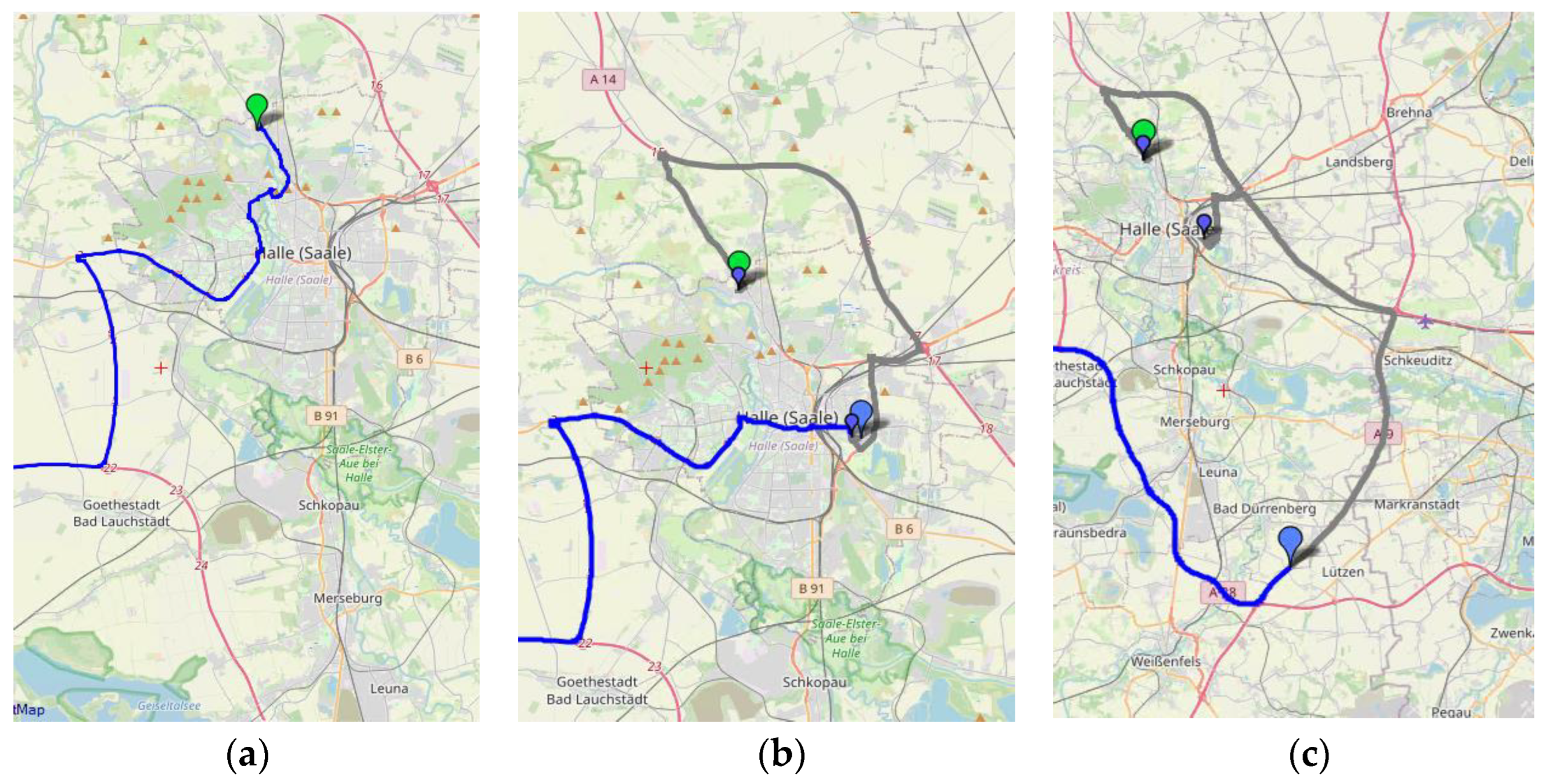
- Initially, it generates vehicle routes based on a given itinerary and draws the planned routes on the road map.
- Next, it looks for the possibilities of reallocating semi-trailers to tractors among the planned routes (switching tractor/semi-trailer compositions) on an hourly basis.
- It simulates the real data arriving from GPS (global positioning system) every hour, updates planned routes, and checks for the possibility of switching tractor/semi-trailer compositions.
- If a switching possibility is found within the maximum deviation from the route (set as parameter), the routes are selected, and the switching point is indicated.
- Next, the new feasible routes are planned, considering that the vehicle compositions must meet each other in the given space and time, while the semi-trailers must follow their itinerary that was originally set.
- Finally, it evaluates the new routes in terms of a savings in the total travel time, and if there is a saving, the routes are displayed on the road map (if there are more possibilities, the best one is indicated).
- Pick-up delay as the difference between the stipulated date of pick-up and the realized date of pick-up, expressed in vehicle workdays, given by Equation (1):where
- PD = total pick-up delay
- DPri = realized date of i-th pick-up
- DPsi = stipulated date of i-th pick-up
- n = total number of events where the stipulated date of pick-up is different from the realized date of pick-up.
- Delivery delay as the difference between the stipulated date of delivery and the realized date of delivery, expressed in vehicle workdays, given by Equation (2):where
- DD = total delivery delay
- DDri = realized date of i-th delivery
- DDsi = stipulated date of i-th delivery
- n = total number of events where the stipulated date delivery is different than the realized date of delivery
- Potential saving is the discrepancy between the planned and the actual number of vehicle workdays spent in realization of the transport routes. Considering pick-up delay a triggering event for the transport route optimization that cannot therefore be retroactively influenced, but necessarily causes future delivery delay, the potential saving of vehicle workdays can be obtained as the total delivery delay decreased by the total pick-up delay, expressed in vehicle workdays, as given by Equation (3):where
- S = potential savings
- DD = total delivery delay
- PD = total pick-up delay.
- Potentially released vehicle compositions refer to the number of vehicle compositions that would have been available for performing additional transport operations if potential savings had been achieved. It means that the same volume of transport operations could have been handled by less vehicle compositions, which would enable the transport company to acquire more transport orders, i.e., to perform more transport operations with the same vehicle fleet. Considering the prescribed working hours of the driver (cf., Figure 1), a vehicle composition can be used a maximum of 24 days a month.
- With reference to the above, the number of vehicle compositions that may be released and used to perform additional transport operations is given by Equation (4):where
- R = number of released vehicles
- S = potential saving (vehicle workdays)
4. Results
4.1. The Case Study
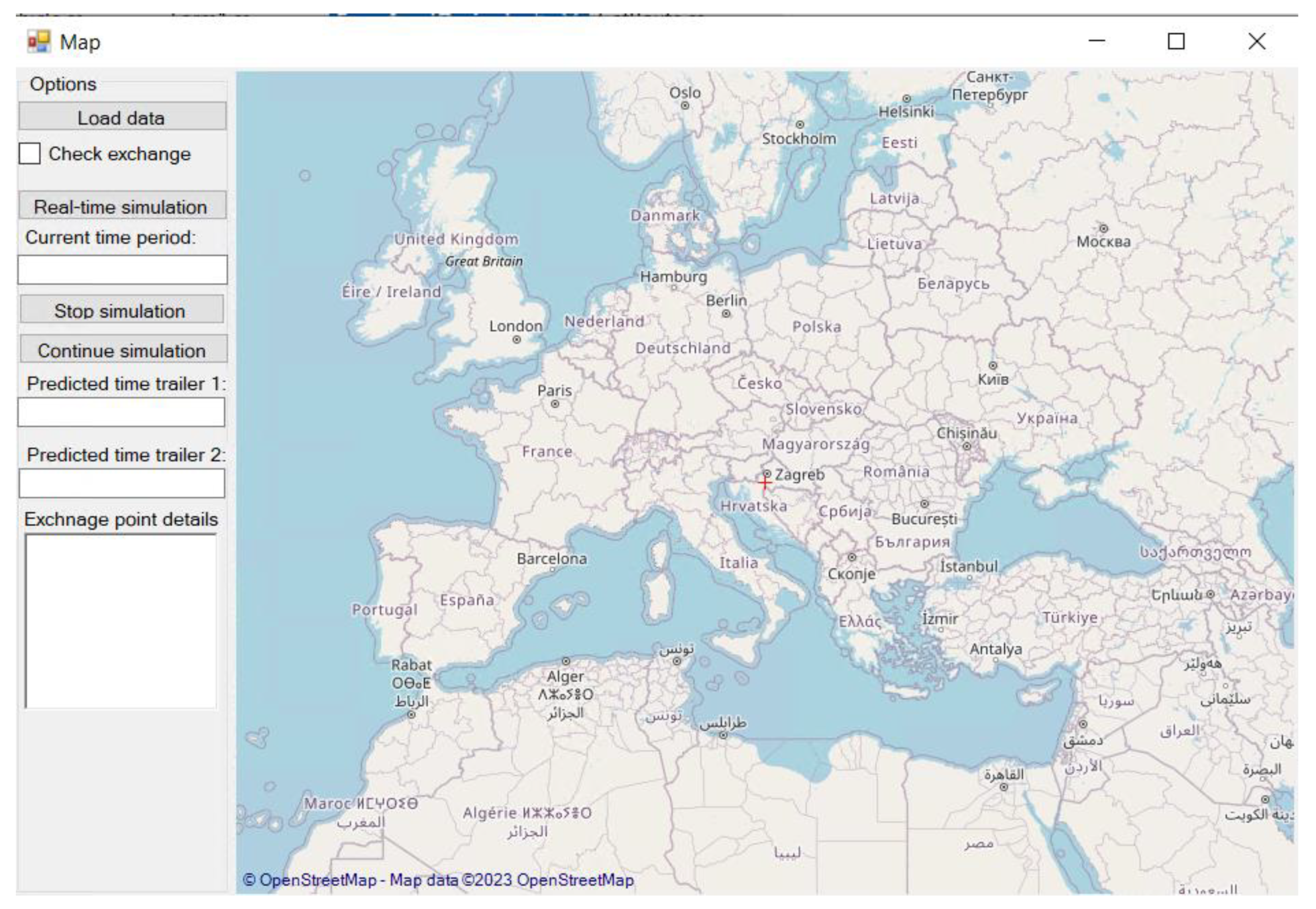
4.2. Simulation Using the Prototype Application
4.2.1. Input Data for the Simulation
4.2.2. Computation of Predicted Routes
4.2.3. Determination of Routing Plan
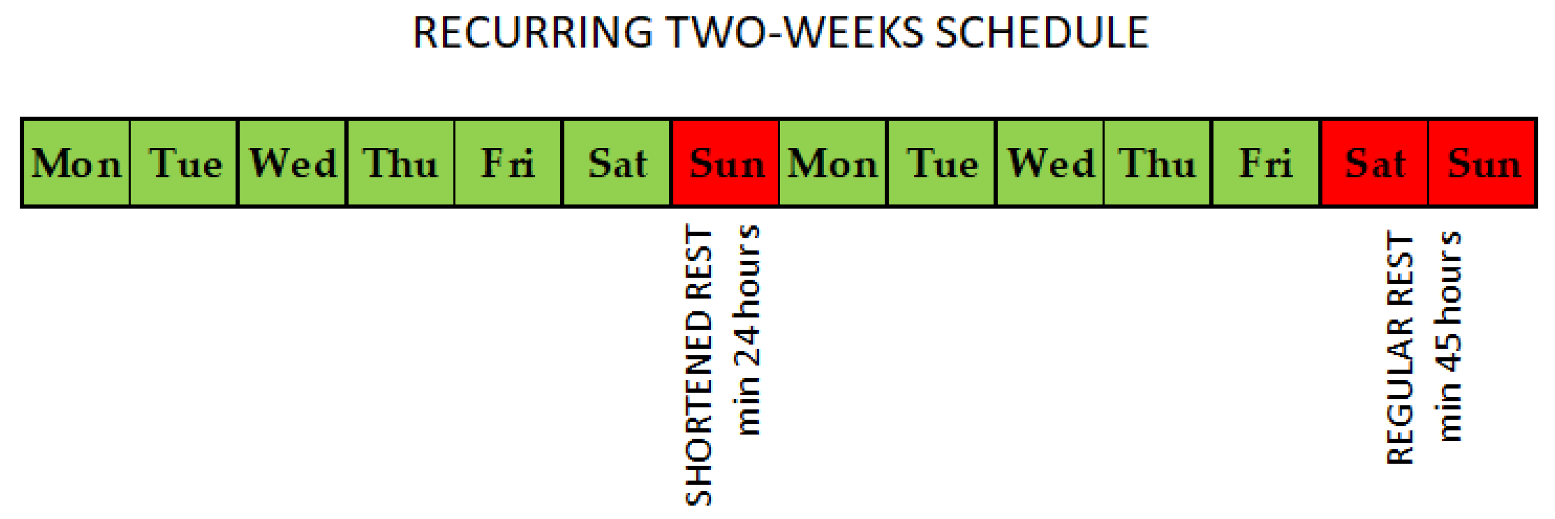
- The maximum daily driving period is 9 h, with an exception allowing it to be extended to 10 h twice a week.
- The total weekly driving time cannot surpass 56 h, and the total fortnightly driving time must not exceed 90 h.
- A daily rest period of at least 11 h is required, with the possibility of reducing it to 9 h up to three times a week. This daily rest can be split into two parts: 3 h followed by 9 h, resulting in a total of 12 h of rest.
- Breaks of at least 45 min, which can be divided into 15 min followed by 30 min, must be taken after driving for a maximum of 4½ hours.
- A weekly rest period should last for 45 continuous hours but can be reduced to 24 h every second week, subject to compensation arrangements. This weekly rest must be taken after six consecutive working days, except for drivers engaged in occasional international passenger transport, who may postpone their weekly rest period for up to 12 days to accommodate holidays.
- In exceptional situations, daily and/or weekly driving times may be exceeded by up to one hour to allow the driver to reach their place of residence or the employer’s operational center to take a weekly rest period.
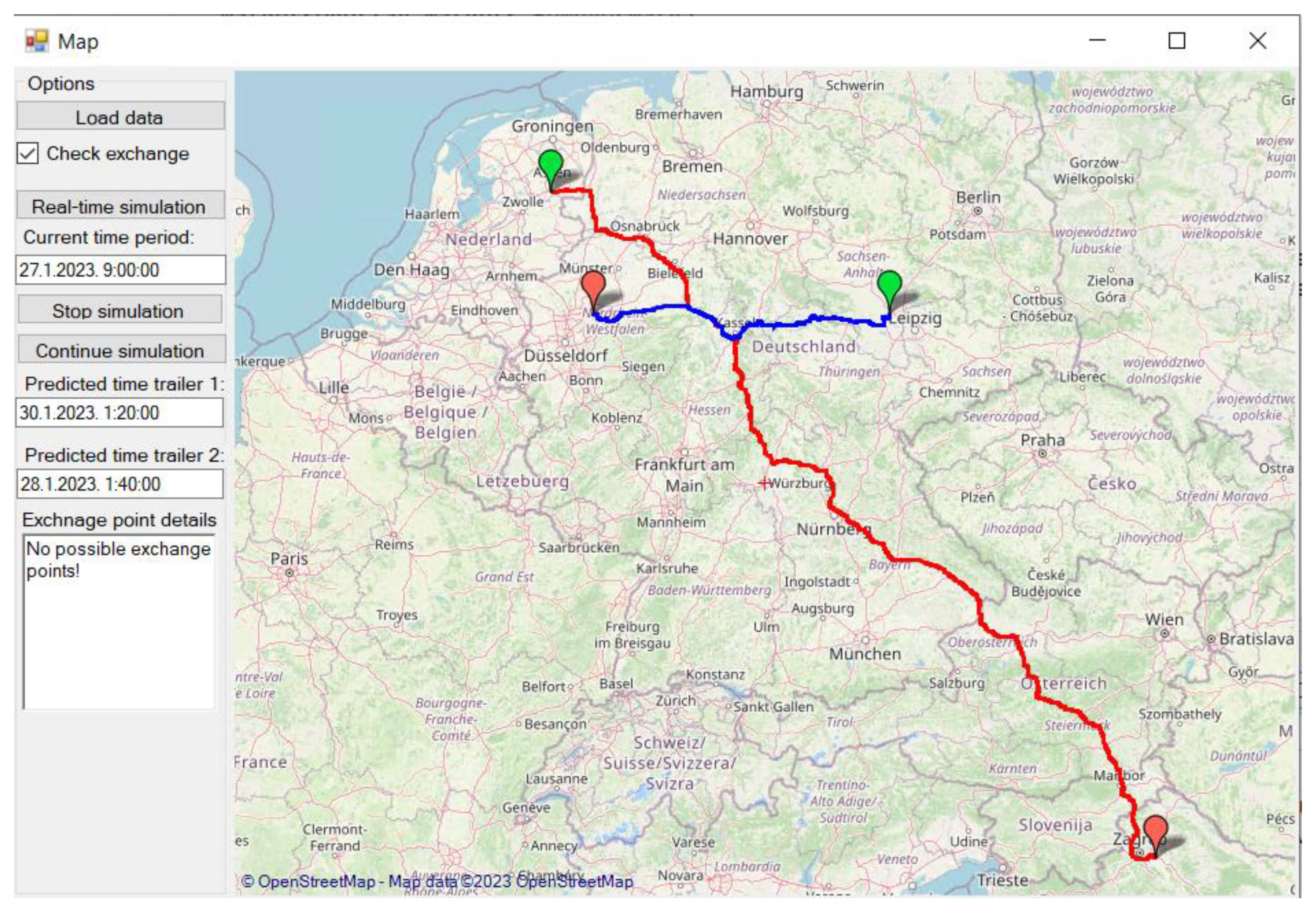
4.2.4. Check for Semi-Trailer Exchange
| Algorithm 1: Evaluate possible exchanges for current routing plan |
| 1. Initialize an empty list to store possible savings 2. For each time bucket in planned horizons: 3. Get the positions of semi-trailers at the current time bucket 4. If semi-trailers are spatially close: 5. Find the closest not visited stop within the threshold for each semi-trailer 6. Compute the exchange point or approximate it as the midpoint 7. Compute new routes from current positions to the exchange points 8. Recompute the rest of the routes with exchanged stops 9. Determine new route planning horizons including driving and rest times 10. Compute end times for semi-trailers 11. Compute the duration savings compared to the no-exchange scenario 12. If savings are possible: 13. Store the pair and the duration savings in the list of possible savings 14. If possible savings is not empty: 15. Identify the pair with the highest total duration savings 16. Store the best exchange in the result |
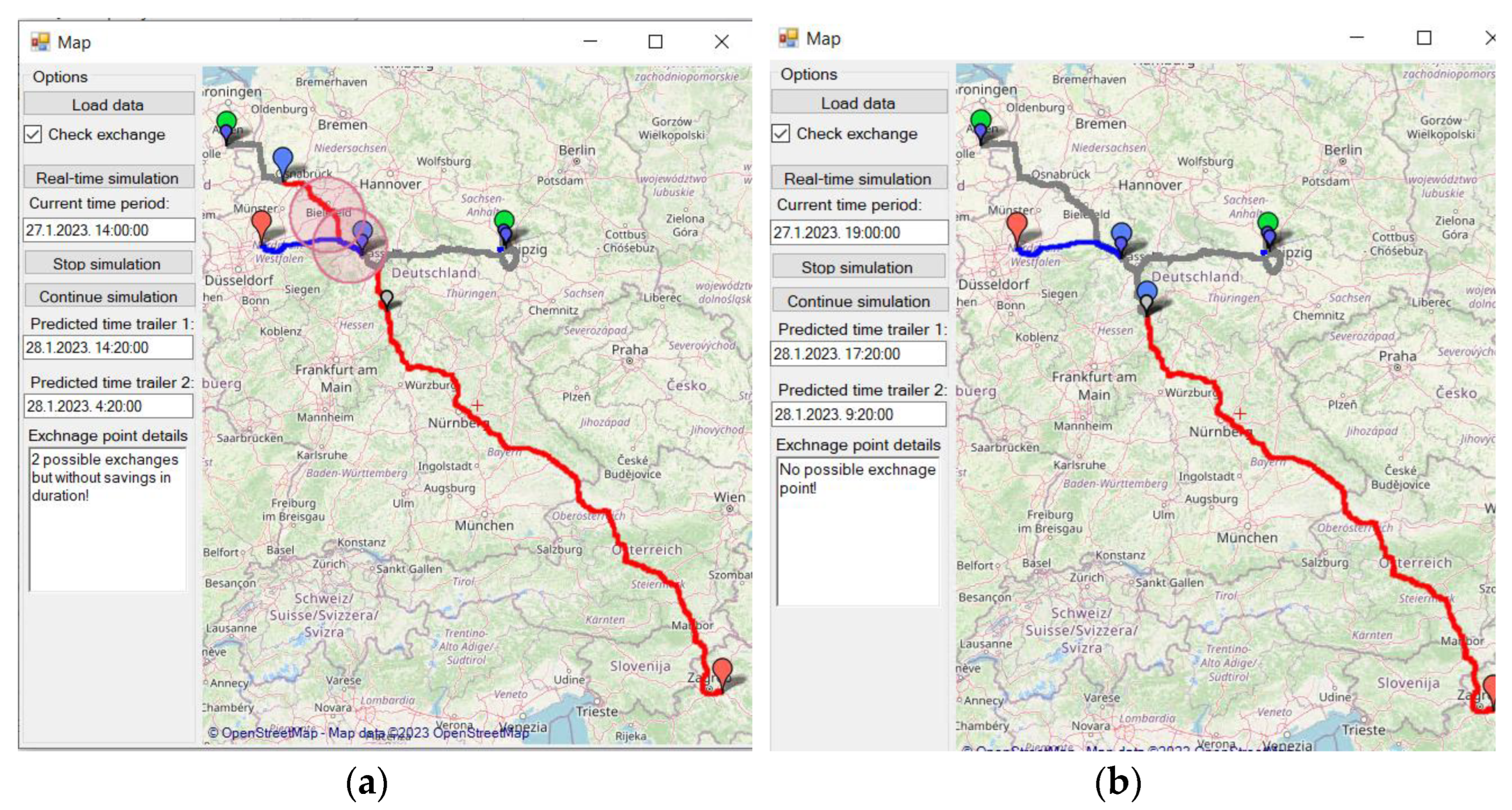
4.2.5. Real-Time Update
- Start time is the current real revealed time
- New predicted routes are computed
- New routing plan is determined
- New exchange points are computed.
4.2.6. Simulation
4.2.7. Sensitivity Analysis
5. Discussion
- (a)
- Reducing the number of vehicle workdays spent performing transport operations (2.16% in this case), which would increase the profitability of transport operations and improve safety of the products being transported.
- (b)
- Reducing the number of vehicle compositions needed to handle the transport demand (2.34% in this case, taking into account average operational availability of the vehicle fleet), which enables the transport company to acquire more transport orders while operating the existing vehicle fleet (increased volume of transport operations).
- (c)
- Improving the quality of the transport service (meeting quality standards) and raising the level of customer satisfaction, by reducing delivery delays.
- (d)
- Better coordination of the transport operations department, that enables dispatchers to handle more transport orders (increased productivity).
- Although in electronic form, transport orders contain location names that require a geocoding service to extract the GPS locations. In addition to departure and destination that are indicated in the transport order, there are other stops on the route that the driver made for some reason, for which the GPS data also need to be retrieved.
- Prior to planning the transport route, accurate information on the driver’s working time in the previous 30 days must be available. This information is essential for route planning, as it is a constraint that defines the approximate locations of stopping points and duration of stays along the route. It has a direct impact on the results of searching the feasible switching points of tractor/semi-trailer compositions on different routes in space and time.
- The planned route and the route driven do not match completely (only after several real-time updates does the match increase) because the drivers may make a detour for some reason.
- In route planning, we were using the free version of the ORS API, which is limited to 40 calls per minute, and 2000 calls per day. In the example outlined in Section 4, it took three minutes to evaluate all the planned routes, as the new updated routes are planned on an hourly basis, when the real-time data is retrieved. Also, when checking the exchange points, the application algorithm needs to define the most suitable deviations from the selected routes to enable vehicles to reach the same location in space and time. Additionally, the rest of the route from the exchange point to the end of the route also needs to be determined. For larger problems, the paid version of some routing service needs to be used.
- The evaluation of switching possibility is carried out if the vehicles are less than 100 km apart in the space-time flow. We set this value as a parameter, which could possibly be increased, as the hourly spatiotemporal discretization of the simulation is rather coarse. We had to do so, in order not to plan routes too frequently and not to overload the ORS server.
- Searching for switching possibilities makes sense if there is a sufficient number of tractor/semi-trailer compositions (the road transport company from the case study operates 140 tractor/semi-trailer compositions). In the conducted case study, we investigated the possible exchange for only two semi-trailers, and not the subset combination from all 140 semi-trailers. There were in total 211 checks for exchange points, and only eight within the 100 km threshold at a specific time. The evaluation of the whole fleet of 140 semi-trailers would significantly increase the search space and execution time, as there are in total possible permutations of a subset of two semi-trailers from the whole 140 semi-trailers in the fleet. Also considering the substantial use of the shortest path algorithm, the final system should definitely use some faster decision algorithms, use a lower discretization period (a couple of hours), or use some form of parallelization.
6. Conclusions
Author Contributions
Funding
Data Availability Statement
Conflicts of Interest
References
- Khan, A.S.; AlArjani, A. A Cold Chain Vehicle Routing Problem Embedded with Manufacturing, Re-Manufacturing and Product Quality under Multiple Constraints. In Proceedings of the 2021 IEEE International Conference on Industrial Engineering and Engineering Management, IEEM, Singapore, 13–16 December 2021; Institute of Electrical and Electronics Engineers Inc.: Piscataway, NJ, USA, 2021; pp. 68–72. [Google Scholar] [CrossRef]
- Cui, J.; Wu, D.; Mansour, R.F. Research on EVRP of Cold Chain Logistics Distribution Based on Improved Ant Colony Algorithm; Lecture Notes in Computer Science (Including Subseries Lecture Notes in Artificial Intelligence and Lecture Notes in Bioinformatics); LNCS:537–48; Springer Science and Business Media Deutschland GmbH: Berlin/Heidelberg, Germany, 2022; Volume 13338. [Google Scholar]
- Fu, M.; Wang, D. Research on Optimization of Cold Chain Logistics Distribution Path of Fresh Products Based on Hybrid Genetic Algorithm. Proc. IOP Conf. Ser. Earth Environ. Sci. 2020, 585, 012131. [Google Scholar] [CrossRef]
- Ji, Y.; Du, J.; Wu, X.; Wu, Z.; Qu, D.; Yang, D. Robust Optimization Approach to Two-Echelon Agricultural Cold Chain Logistics Considering Carbon Emission and Stochastic Demand. Environ. Dev. Sustain. 2021, 23, 13731–13754. [Google Scholar] [CrossRef]
- Jia, X. Research on the Optimization of Cold Chain Logistics Distribution Path of Agricultural Products E-Commerce in Urban Ecosystem from the Perspective of Carbon Neutrality. Front. Ecol. Evol. 2022, 10, 966111. [Google Scholar] [CrossRef]
- Wu, D.; Cui, J.; Li, D.; Mansour, R.F. A New Route Optimization Approach of Fresh Agricultural Logistics Distribution. Intell. Autom. Soft Comput. 2022, 34, 1553–1569. [Google Scholar] [CrossRef]
- Wu, L.J.; Chen, Z.G.; Chen, C.H.; Li, Y.; Jeon, S.W.; Zhang, J.; Zhan, Z.H. Real Environment-Aware Multisource Data-Associated Cold Chain Logistics Scheduling: A Multiple Population-Based Multiobjective Ant Colony System Approach. IEEE Trans. Intell. Transp. Syst. 2022, 23, 23613–23627. [Google Scholar] [CrossRef]
- Wu, X.; Hu, D.; Liu, C. Optimization of Vehicle Routing Problem in Cold Chain Logistics under Low Carbon Economy. In Proceedings of the 19th COTA International Conference of Transportation Professionals, Nanjing, China, 6–8 July 2019; pp. 4551–4563. [Google Scholar]
- Yao, Q.; Zhu, S.; Li, Y. Green Vehicle-Routing Problem of Fresh Agricultural Products Considering Carbon Emission. Int. J. Environ. Res. Public Health 2022, 19, 8675. [Google Scholar] [CrossRef] [PubMed]
- Amaruchkul, K.; Pongsathornwiwat, A.; Bantadtiang, P. Constrained Joint Replenishment Problem with Refrigerated Vehicles. Eng. J. 2022, 26, 75–91. [Google Scholar] [CrossRef]
- Golestani, M.; Moosavirad, S.H.; Asadi, Y.; Biglari, S. A Multi-Objective Green Hub Location Problem with Multi Item-Multi Temperature Joint Distribution for Perishable Products in Cold Supply Chain. Sustain. Prod. Consum. 2021, 27, 1183–1194. [Google Scholar] [CrossRef]
- Rahman, H.; Rahman, F.; Tseng, T.L. Estimation of Fuel Consumption and Selection of the Most Carbon-Efficient Route for Cold-Chain Logistics. Int. J. Syst. Sci. Oper. Logist. 2022, 10, 2075043. [Google Scholar] [CrossRef]
- Huai, C.-X.; Sun, G.-H.; Ran-ran, Q.; Gao, Z.; Zhabg, Z.-H. Vehicle Routing Problem with Multi-Type Vehicles in the Cold Chain Logistics System. In Proceedings of the 16th International Conference on Service Systems and Service Management (ICSSSM2019), Shenzhen, China, 13–15 July 2019. [Google Scholar]
- Qi, C.; Hu, L. Optimization of Vehicle Routing Problem for Emergency Cold Chain Logistics Based on Minimum Loss. Phys. Commun. 2020, 40, 101085. [Google Scholar] [CrossRef]
- Song, M.X.; Li, J.Q.; Han, Y.Q.; Han, Y.Y.; Liu, L.L.; Sun, Q. Metaheuristics for Solving the Vehicle Routing Problem with the Time Windows and Energy Consumption in Cold Chain Logistics. Appl. Soft Comput. 2020, 95, 106561. [Google Scholar] [CrossRef]
- Al Theeb, N.; Smadi, H.J.; Al-Hawari, T.H.; Aljarrah, M.H. Optimization of Vehicle Routing with Inventory Allocation Problems in Cold Supply Chain Logistics. Comput. Ind. Eng. 2020, 142, 106341. [Google Scholar] [CrossRef]
- Wang, Z.; Wen, P. Optimization of a Low-Carbon Two-Echelon Heterogeneous-Fleet Vehicle Routing for Cold Chain Logistics under Mixed Time Window. Sustainability 2020, 12, 1967. [Google Scholar] [CrossRef]
- Zhang, Y.; Hua, G.; Cheng, T.C.E.; Zhang, J. Cold Chain Distribution: How to Deal with Node and Arc Time Windows? Ann. Oper. Res. 2020, 291, 1127–1151. [Google Scholar] [CrossRef]
- Zhao, B.; Gui, H.; Li, H.; Xue, J. Cold Chain Logistics Path Optimization via Improved Multi-Objective Ant Colony Algorithm. IEEE Access 2020, 8, 142977–142995. [Google Scholar] [CrossRef]
- Zhao, Z.; Li, X.; Zhou, X. Distribution Route Optimization for Electric Vehicles in Urban Cold Chain Logistics for Fresh Products under Time-Varying Traffic Conditions. Math. Probl. Eng. 2020, 2020, 9864935. [Google Scholar] [CrossRef]
- Zhu, S.; Fu, H.; Li, Y. Optimization Research on Vehicle Routing for Fresh Agricultural Products Based on the Investment of Freshness-Keeping Cost in the Distribution Process. Sustainability 2021, 13, 8110. [Google Scholar] [CrossRef]
- Jiao, X.; Xu, W.; Duan, L. Study on Cold Chain Transportation Model of Fruit and Vegetable Fresh-Keeping in Low-Temperature Cold Storage Environment. Discret. Dyn. Nat. Soc. 2021, 2021, 8445028. [Google Scholar] [CrossRef]
- Li, F.; Ai, W.; Ju, T. Cold Chain Logistics Distribution Path Planning of Fresh Products in Beijing Subcenter. Sustainability 2022, 14, 10622. [Google Scholar] [CrossRef]
- Lim, M.K.; Li, Y.; Song, X. Exploring Customer Satisfaction in Cold Chain Logistics Using a Text Mining Approach. Ind. Manag. Data Syst. 2021, 121, 2426–2449. [Google Scholar] [CrossRef]
- Rahbari, M.; Hajiagha, S.H.R.; Mahdiraji, H.A.; Dorcheh, F.R.; Garza-Reyes, J.A. Internal A Novel Location-Inventory-Routing Problem in a Two-Stage Red Meat Supply Chain with Logistic Decisions: Evidence from an Emerging Economy A Novel Location-Inventory-Routing Problem in a Two-Stage Red Meat Supply Chain with Logistic Decisions: Evidence from an Emerging Economy. Kybernetes 2022, 51, 1498–1531. [Google Scholar]
- Wang, M.; Wang, Y.; Liu, W.; Ma, Y.; Xiang, L.; Yang, Y.; Li, X. How to Achieve a Win–Win Scenario between Cost and Customer Satisfaction for Cold Chain Logistics? Phys. A Stat. Mech. Its Appl. 2021, 566, 125637. [Google Scholar] [CrossRef]
- Wu, D.; Zhu, Z.; Hu, D.; Mansour, R.F. Optimizing Fresh Logistics Distribution Route Based on Improved Ant Colony Algorithm. Comput. Mater. Contin. 2022, 73, 2079–2095. [Google Scholar] [CrossRef]
- Yang, Y.; Zang, Y.; Qi, M. Robust Network Design and Last-Mile Delivery in Cold Chain Logistics System. In Proceedings of the 2021 IEEE International Conference on Industrial Engineering and Engineering Management, IEEE 2021, Singapore, 13–16 December 2021; Institute of Electrical and Electronics Engineers Inc.: Piscataway, NJ, USA, 2021; pp. 765–772. [Google Scholar] [CrossRef]
- Zhou, L.; Li, Q.; Li, F.; Jin, C. Research on Green Technology Path of Cold-Chain Distribution of Fresh Products Based on Sustainable Development Goals. Sustainability 2022, 14, 16659. [Google Scholar] [CrossRef]
- Bai, Q.; Yin, X.; Lim, M.K.; Dong, C. Low-Carbon VRP for Cold Chain Logistics Considering Real-Time Traffic Conditions in the Road Network. Ind. Manag. Data Syst. 2022, 122, 521–543. [Google Scholar] [CrossRef]
- Chen, Y.; Lan, H.; Wang, C.; Jia, X. Integrated Online Order Picking and Vehicle Routing of Food Cold Chain with Demand Surge. Math. Probl. Eng. 2022, 2022, 4485376. [Google Scholar] [CrossRef]
- Dávila, S.; Alfaro, M.; Fuertes, G.; Vargas, M.; Camargo, M. Vehicle Routing Problem with Deadline and Stochastic Service Times: Case of the Ice Cream Industry in Santiago City of Chile. Mathematics 2021, 9, 2750. [Google Scholar] [CrossRef]
- Fu, Z.; Dong, P.; Ju, Y. An Intelligent Green Vehicle Management System for Urban Food Re-liably Delivery: A Case Study of Shanghai, China. Energy 2022, 257, 124642. [Google Scholar] [CrossRef]
- Hu, L.; Xiang, C.; Qi, C. Optimization of VRR for Cold Chain with Minimum Loss Based on Actual Traffic Conditions. Wirel. Commun. Mob. Comput. 2021, 2021, 2930366. [Google Scholar] [CrossRef]
- Leng, L.; Zhang, C.; Zhao, Y.; Wang, W.; Zhang, J.; Li, G. Biobjective Low-Carbon Location-Routing Problem for Cold Chain Logistics: Formulation and Heuristic Approaches. J. Clean. Prod. 2020, 273, 122801. [Google Scholar] [CrossRef]
- Leng, L.; Zhang, J.; Zhang, C.; Zhao, Y.; Wang, W.; Li, G. A Novel Bi-Objective Model of Cold Chain Logistics Considering Location-Routing Decision and Environmental Effects. PLoS ONE 2020, 15, e0230867. [Google Scholar] [CrossRef] [PubMed]
- Li, D.; Cao, Q.; Zuo, M.; Xu, F. Optimization of Green Fresh Food Logistics with Heterogeneous Fleet Vehicle Route Problem by Improved Genetic Algorithm. Sustainability 2020, 12, 1946. [Google Scholar] [CrossRef]
- Liu, C.; Zhang, Z.; Su, X.; Qin, H. A Hybrid Algorithm for the Vehicle Routing Problem with Compatibility Constraints. In Proceedings of the ICNSC 2018—15th IEEE International Conference on Networking, Sensing and Control, Zhuhai, China, 27–29 March 2018; Institute of Electrical and Electronics Engineers Inc.: Piscataway, NJ, USA, 2018. [Google Scholar] [CrossRef]
- Shi, Y.; Lin, Y.; Lim, M.K.; Tseng, M.-L.; Tan, C.; Li, Y. An Intelligent Green Scheduling System for Sustainable Cold Chain Logistics. Expert Syst. Appl. 2022, 209, 118378. [Google Scholar] [CrossRef]
- Wang, H.; Li, W.; Li, M.; Yang, X.; Wang, Z.; Zhao, Z.; Wang, L. Intelligent Selection of Delivery Parties for Fresh Agricultural Product Based on Third-Party Logistics in Smart City. Sustain. Energy Technol. Assess. 2022, 52, 102151. [Google Scholar] [CrossRef]
- Yu, L. A route optimization model based on cold chain logistics distribution for fresh agricultural products from a low-carbon perspective. Fresenius Environ. Bull. 2021, 30, 1112–1124. [Google Scholar]
- Khan, A.S.; Salah, B.; Zimon, D.; Ikram, M.; Khan, R.; Pruncu, C.I. A Sustainable Distribution Design for Multi-Quality Multiple-Cold-Chain Products: An Integrated Inspection Strategies Approach. Energies 2020, 13, 6612. [Google Scholar] [CrossRef]
- Maiorino, A.; Petruzziello, F.; Aprea, C. Refrigerated Transport: State of the Art, Technical Issues, Innovations and Challenges for Sustainability. Energies 2021, 14, 7237. [Google Scholar] [CrossRef]
- Suraraksa, J.; Shin, K.S. Urban Transportation Network Design for Fresh Fruit and Vegetables Using Gis–the Case of Bangkok. Appl. Sci. 2019, 9, 5048. [Google Scholar] [CrossRef]
- Yan, L.; Grifoll, M.; Zheng, P. Model and Algorithm of Two-Stage Distribution Location Routing with Hard Time Window for City Cold-Chain Logistics. Appl. Sci. 2020, 10, 2564. [Google Scholar] [CrossRef]
- Ba, Y.; Feng, C.; Jia, W.; Liu, X.; Ren, J. A Multi-Scenario Optimization Model for Emergency Cold Chain Logistics Distribution. Math. Probl. Eng. 2021, 2021, 1628162. [Google Scholar] [CrossRef]
- Chen, J.; Liao, W.; Yu, C. Route optimization for Cold Chain Logistics of Front Warehouses Based on Traffic Congestion and Carbon Emission. Comput. Ind. Eng. 2021, 161, 107663. [Google Scholar] [CrossRef]
- Chen, J.; Gui, P.; Ding, T.; Na, S.; Zhou, Y. Optimization of Transportation Routing Problem for Fresh Food by Improved Ant Colony Algorithm Based on Tabu Search. Sustainability 2019, 11, 6584. [Google Scholar] [CrossRef]
- Chen, Y.; Lan, H.; Wang, C.; Jia, X. An integrated distribution scheduling and route planning of food cold chain with demand surge. Complex Intell. Syst. 2023, 9, 475–491. [Google Scholar] [CrossRef] [PubMed]
- Guo, N.; Qian, B.; Na, J.; Hu, R.; Mao, J.-L. A Three-Dimensional Ant Colony Optimization Algorithm for Multi-Compartment Vehicle Routing Problem Considering Carbon Emissions. Appl. Soft Comput. 2022, 127, 109326. [Google Scholar] [CrossRef]
- Lian, J. An Optimization Model of Cross-Docking Scheduling of Cold Chain Logistics Based on Fuzzy Time Window. J. Intell. Fuzzy Syst. 2021, 41, 1901–1915. [Google Scholar] [CrossRef]
- Liu, G.; Hu, J.; Yang, Y.; Xia, S.; Lim, M.K. Vehicle Routing Problem in Cold Chain Logistics: A Joint Distribution Model with Carbon Trading Mechanisms. Resour. Conserv. Recycl. 2020, 156, 104715. [Google Scholar] [CrossRef]
- Liu, S.; Zhang, C. Optimization of Urban Cold Chain Transport Routes under Time-Varying Network Conditions. J. Adv. Transp. 2021, 2021, 8817991. [Google Scholar] [CrossRef]
- Liu, S.; Zhang, C. Optimization of Cold Chain Distribution Route with Mixed Time Window Considering Customer Priority. Comput. Intell. Neurosci. 2022, 2022, 2953205. [Google Scholar] [CrossRef]
- Qiao, J. Research on Optimizing the Distribution Route of Food Cold Chain Logistics Based on Modern Biotechnology. AIP Conf. Proc. 2019, 2110, 020070. [Google Scholar] [CrossRef]
- Qin, G.; Tao, F.; Li, L. A Vehicle Routing Optimization Problem for Cold Chain Logistics Considering Customer Satisfaction and Carbon Emissions. Int. J. Environ. Res. Public Health 2019, 16, 576. [Google Scholar] [CrossRef]
- Ren, X.Y. Path Optimization of Cold Chain Distribution with Multiple Distribution Centers Considering Carbon Emissions. Appl. Ecol. Environ. Res. 2019, 17, 9437–9453. [Google Scholar] [CrossRef]
- Tsang, Y.P.; Choy, K.L.; Wu, C.H.; Ho, G.T.S.; Lam, H.Y.; Tang, V. An Intelligent Model for Assuring Food Quality in Managing a Multi-Temperature Food Distribution Centre. Food Control 2018, 90, 81–97. [Google Scholar] [CrossRef]
- Wang, Y.; Yang, C.; Hou, H. Risk Management in Perishable Food Distribution Operations. Ind. Manag. Data Syst. 2020, 120, 291–311. [Google Scholar] [CrossRef]
- Wu, L.-J.; Shi, L.; Zhan, Z.-H.; Lai, K.-K.; Zhang, J. A Buffer-Based Ant Colony System Approach for Dynamic Cold Chain Logistics Scheduling. IEEE Trans. Emerg. Top. Comput. Intell. 2022, 6, 1438–1452. [Google Scholar] [CrossRef]
- Xie, Y.; Li, Y. Optimizing Method of Cold Link Path for Agricultural Products Transportation Facing Environmental Protection. Ekoloji 2019, 28, 2083–2095. [Google Scholar]
- Xiong, H. Research on Cold Chain Logistics Distribution Route Based on Ant Colony Optimization Algorithm. Discret. Dyn. Nat. Soc. 2021, 2021, 6623563. [Google Scholar] [CrossRef]
- Yu, H. Research on Fresh Product Logistics Transportation Scheduling Based on Deep Reinforcement Learning. Sci. Program. 2022, 2022, 8750580. [Google Scholar] [CrossRef]
- Zhang, B. The Optimization of Distribution Path of Fresh Cold Chain Logistics Based on Genetic Algorithm. Comput. Intell. Neurosci. 2022, 2022, 4667010. [Google Scholar] [CrossRef]
- Zulvia, F.E.; Kuo, R.; Nugroho, D.Y. A Many-Objective Gradient Evolution Algorithm for Solving a Green Vehicle Routing Problem with Time Windows and Time Dependency for Perishable Products. J. Clean. Prod. 2020, 242, 118428. [Google Scholar] [CrossRef]
- Fu, Q.; Li, J.; Chen, H. Resource Scheduling Method for Optimizing the Distribution Path of Fresh Agricultural Products under Low-Carbon Environmental Constraints. Sci. Program. 2022, 2022, 7692135. [Google Scholar] [CrossRef]
- Li, N.; Li, G. Hybrid Partheno-Genetic Algorithm for Multi-Depot Perishable Food Delivery Problem with Mixed Time Windows. Ann. Oper. Res. 2022, 312, 1–32. [Google Scholar] [CrossRef]
- Lim, M.K.; Li, Y.; Wang, C.; Tseng, M.-L. Prediction of Cold Chain Logistics Temperature Using a Novel Hybrid Model Based on the Mayfly Algorithm and Extreme Learning Machine. Ind. Manag. Data Syst. 2022, 122, 819–840. [Google Scholar] [CrossRef]
- Qiang, X.; Appiah, M.Y.; Boateng, K.; Appiah, F.V. Route Optimization Cold Chain Logistic Distribution Using Greedy Search Method. Opsearch 2020, 57, 1115–1130. [Google Scholar] [CrossRef]
- Utama, D.M.; Widodo, D.S.; Ibrahim, M.F.; Dewi, S.K. A New Hybrid Butterfly Optimization Algorithm for Green Vehicle Routing Problem. J. Adv. Transp. 2020, 2020, 8834502. [Google Scholar] [CrossRef]
- Yan, L.; Zheng, P. Study on Vehicle Routing Optimization of Cold Chain Logistics with Soft Time Window under Stochastic Demand. UPB Sci. Bull. 2020, 82. [Google Scholar]
- Huiling, Z.; Dinglan, W.; Changgui, L.; Yanchun, W. Research on Optimization of Pasteurized Milk Cold Chain Logistics Distribution Network. In Proceedings of the 2018 15th International Conference on Service Systems and Service Management, ICSSSM 2018, Hangzhou, China, 21–22 July 2018; Institute of Electrical and Electronics Engineers Inc.: Piscataway, NJ, USA, 2018. [Google Scholar] [CrossRef]
- Zhao, Z.; Li, X.; Zhou, X. Optimization of Transportation Routing Problem for Fresh Food in Time-Varying Road Network: Considering Both Food Safety Reliability and Temperature Control. PLoS ONE 2020, 15, e0235950. [Google Scholar] [CrossRef] [PubMed]
- Ivan, D.W.; Vanany, I.; Siswanto, N. An Optimization Model for Fresh-Food Electronic Commerce Supply Chain with Carbon Emissions and Food Waste. J. Ind. Prod. Eng. 2022, 40, 1–21. [Google Scholar]
- Ning, T.; An, L.; Duan, X. Optimization of Cold Chain Distribution Path of Fresh Agricultural Products under Carbon Tax Mechanism: A Case Study in China. J. Intell. Fuzzy Syst. 2021, 40, 10549–10558. [Google Scholar] [CrossRef]
- Shui, W.; Li, M. Integrated Pricing and Distribution Planning for Community Group Purchase of Fresh Agricultural Products. Sci. Program. 2020, 2020, 8839398. [Google Scholar] [CrossRef]
- Li, Y.; Lim, M.K.; Tseng, M.-L. A Green Vehicle Routing Model Based on Modified Particle Swarm Optimization for Cold Chain Logistics. Ind. Manag. Data Syst. 2019, 119, 473–494. [Google Scholar] [CrossRef]
- Chaudhuri, A.; Dukovska-Popovska, I.; Subramanian, N.; Chan, H.K.; Bai, R. Decision-making in cold chain logistics using data analytics: A literature review. Int. J. Logist. Manag. 2018, 29, 839–861. [Google Scholar] [CrossRef]
- Kadlubek, M. Completeness Meter in Logistics Service Quality Management of Transport Companies. Int. J. Qual. Res. 2020, 14, 1223–1234. [Google Scholar] [CrossRef]
- Kadłubek, M.; Jereb, B. Measurement of the Logistic Customer Service Level in Commercial Cargo Motor Transport Companies. Logist. Sustain. Transp. 2014, 5, 8–15. [Google Scholar] [CrossRef]
- Yue, J.; Liu, L.; Li, Z.; Li, D.; Fu, Z. Improved Quality Analytical Models for Aquatic Products at the Transportation in the Cold Chain. Math. Comput. Model. 2013, 58, 474–479. [Google Scholar] [CrossRef]
- Bauer, R.; Delling, D.; Sanders, P.; Schieferdecker, D.; Schultes, D.; Wagner, D. Combining hierarchical and goal-directed speed-up techniques for dijkstra’s algorithm. ACM J. Exp. Algorithmics 2010, 15, 2.1–2.31. [Google Scholar] [CrossRef]
- European Commisson. Mobility and Transport—Driving Time and Rest Periods. Available online: https://transport.ec.europa.eu/transport-modes/road/social-provisions/driving-time-and-rest-periods_en (accessed on 28 June 2023).


| Reference | Transport Costs | Quality and Safety | Environmental Impact | Customer Satisfaction |
|---|---|---|---|---|
| [1] | ✓ | ✓ | ✓ | ✓ |
| [2,3,4,5,6,7,8,9] | ✓ | ✓ | ✓ | |
| [10,11,12,13,14,15,16,17,18,19,20,21] | ✓ | ✓ | ||
| [22,23,24,25,26,27,28,29] | ✓ | ✓ | ✓ | |
| [30,31,32,33,34,35,36,37,38,39,40,41] | ✓ | ✓ | ||
| [42,43,44,45] | ✓ | ✓ | ||
| [46,47,48,49,50,51,52,53,54,55,56,57,58,59,60,61,62,63,64,65] | ✓ | |||
| [66] | ✓ | ✓ | ||
| [67,68,69,70,71,72] | ✓ | |||
| [73] | ✓ | ✓ | ||
| [74,75,76] | ✓ | |||
| [77] | ✓ |
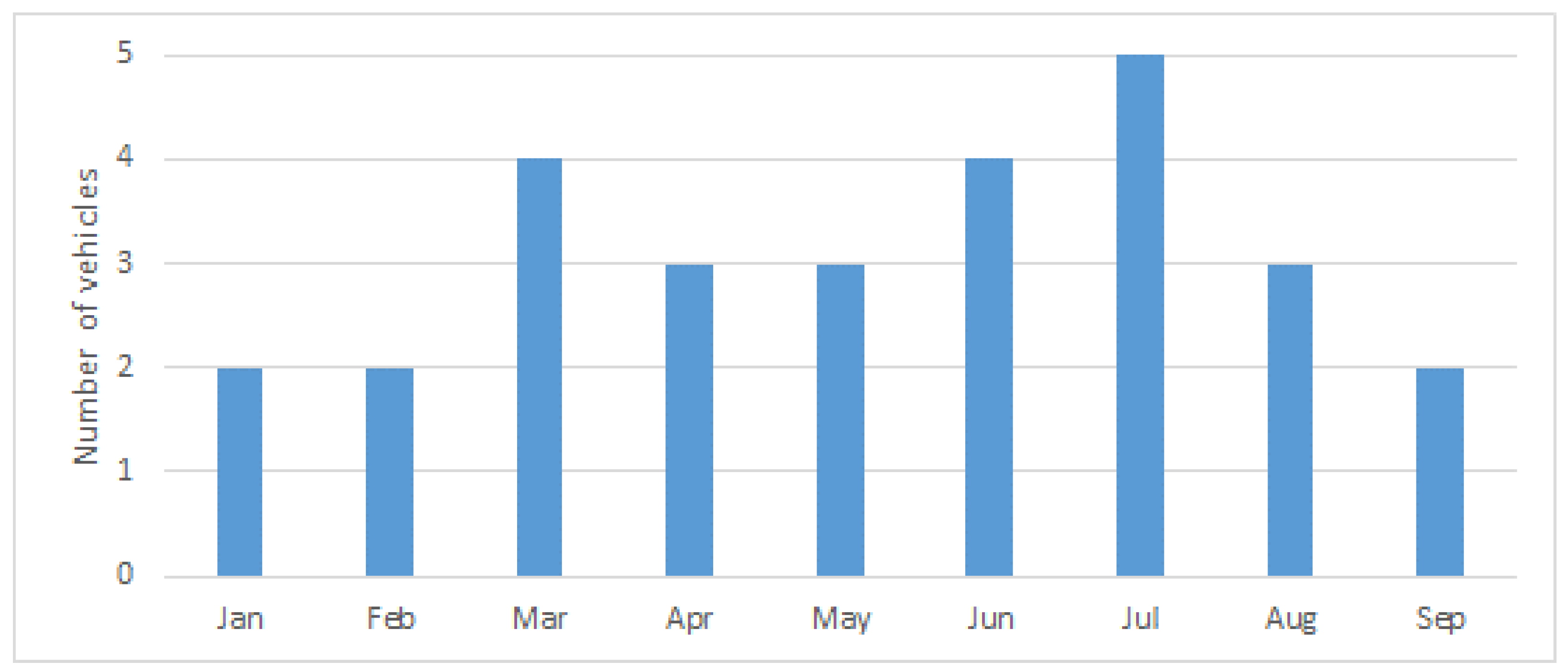
| Month in 2023 | Number of Transport Orders | Number of Transport Routes | Average Number of Orders per Route | Average Duration of Transport Route (Days) |
|---|---|---|---|---|
| Jan | 1651 | 507 | 3.3 | 8.3 |
| Feb | 1655 | 470 | 3.5 | 8.4 |
| Mar | 1900 | 510 | 3.7 | 8.4 |
| Apr | 1680 | 437 | 3.8 | 9.1 |
| May | 1892 | 528 | 3.6 | 8.1 |
| Jun | 1858 | 513 | 3.6 | 8.4 |
| Jul | 1821 | 518 | 3.5 | 8.3 |
| Aug | 1887 | 500 | 3.8 | 8.3 |
| Sep | 1758 | 450 | 3.9 | 9.4 |
Disclaimer/Publisher’s Note: The statements, opinions and data contained in all publications are solely those of the individual author(s) and contributor(s) and not of MDPI and/or the editor(s). MDPI and/or the editor(s) disclaim responsibility for any injury to people or property resulting from any ideas, methods, instructions or products referred to in the content. |
© 2023 by the authors. Licensee MDPI, Basel, Switzerland. This article is an open access article distributed under the terms and conditions of the Creative Commons Attribution (CC BY) license (https://creativecommons.org/licenses/by/4.0/).
Share and Cite
Stanković, R.; Pereglin, T.; Erdelić, T. Optimizing Utilization of Transport Capacities in the Cold Chain by Introducing Dynamic Allocation of Semi-Trailers. Logistics 2023, 7, 101. https://doi.org/10.3390/logistics7040101
Stanković R, Pereglin T, Erdelić T. Optimizing Utilization of Transport Capacities in the Cold Chain by Introducing Dynamic Allocation of Semi-Trailers. Logistics. 2023; 7(4):101. https://doi.org/10.3390/logistics7040101
Chicago/Turabian StyleStanković, Ratko, Tomislav Pereglin, and Tomislav Erdelić. 2023. "Optimizing Utilization of Transport Capacities in the Cold Chain by Introducing Dynamic Allocation of Semi-Trailers" Logistics 7, no. 4: 101. https://doi.org/10.3390/logistics7040101
APA StyleStanković, R., Pereglin, T., & Erdelić, T. (2023). Optimizing Utilization of Transport Capacities in the Cold Chain by Introducing Dynamic Allocation of Semi-Trailers. Logistics, 7(4), 101. https://doi.org/10.3390/logistics7040101