A Model for Demand Planning in Supply Chains with Congestion Effects

Abstract

This paper is concerned with demand planning for internal supply chains consisting of workstations, production facilities, warehouses, and transportation links. We address the issue of how to help a supplier firmly accept orders and subsequently plan to fulfill demand. We first formulate a linear aggregate planning model for demand management that incorporates elements of order promising, recipe run constraints, and capacity limitations. Using several scenarios, we discuss the use of the model in demand planning and capacity planning to help a supplier firmly respond to requests for quotations. We extend the model to incorporate congestion effects at assembly and blending nodes using clearing functions; the resulting model is nonlinear. We develop and test two algorithms to solve the nonlinear model: one based on inner approximation and the other on outer approximation.

1. Introduction and Literature Review

The tremendous growth of electronic commerce has focused the attention of supplier firms on the need for both internal and external supply chain integration. To be competitive, it is now necessary not only to synchronize the activities of one’s own internal supply chain, but also to develop and manage a partnership with external business partners and customers. Beamon [1] notes that there has been increasing attention paid to the performance, design, and analysis of the supply chain as a whole. Keskinocak and Tayur [2] discuss the role of quantitative models in the electronic commerce context. Customers have more power and more complex requirements in such a context, which makes flexibility and customer satisfaction the two major concerns in production–distribution system planning. Thus, supply chain firms are moving toward customer-oriented planning and decision-making systems (Askin and Goldberg [3]).

Electronic commerce also makes external supply chain integration possible. External supply chain integration includes negotiation-based due dates and price setting. High-speed internet connections allow instant information exchange between supply chain entities, and consequently reduce transaction costs. A firm can work on the due dates, configuration, and price of products together with its business partners for mutual benefit. An internal integration plan is frequently updated as a result of negotiations, while at the same time providing feedback that impacts the negotiation process itself. Taken to the extreme, the electronic commerce context can allow a firm to establish a seamless interface with its external supply chain.

This paper draws on several streams in the literature. The first stream is concerned with multi-plant coordination and material requirements planning (MRP) systems modelled at the aggregate level. Billington et al. [4] develop mathematical formulations for a multi-stage capacity-constrained MRP system. Baker [5] reviews optimization models in the MRP context, stating that capacity planning is one of the key weaknesses of the MRP framework and should be done in parallel rather than in sequence with material planning. Rota et al. [6] develop linear and mixed integer programming (MIP) formulation of a multi-stage capacity-constrained MRP system, taking into account firm order forecasts and supplier behaviour. While the concept of bill of material is fundamental to assembly systems, many production–distribution models have ignored this issue. Vidal and Goetschaalckx [7] point out that most of the models they review do not include bill-of-material constraints. The models that combine bill-of-material constraints are formulated mainly as MIP in the literature. Arntzen et al. [8] develop an MIP production–distribution model with bill-of-material constraints. Jang et al. [9] present a four-module MIP production–distribution model with bill-of-material constraints. The model we formulate in this paper explicitly considers bill-of-material constraints and simultaneously addresses capacity planning and materials planning.

The second stream of research that we draw on is that of demand management. Demand management is involved with the transfer of demand data, combined from forecasting, committed orders, and ongoing negotiation, to the production system for different levels of planning to ensure demands are met (Shapiro [10]). Order promising is the function within demand management in which firms quote (and subsequently commit to) due dates and prices. For a firm to quote prices, it should have as precise an estimate of costs as possible. Since prices and due dates are generally negotiable, the literature on negotiation in the supply chain context is also relevant. Rosenfield et al. [11] hypothesize that the shape of the cost versus lead time trade-off curve is a function of four key variables: the nature of demand, product variety, the economics of transportation, and the structure of the value-added chain. From a supplier firm’s contractual viewpoint, total cost decreases with longer delivery time. Moodie and Bobrowski [12] study the due date versus price trade-off curve from an operational perspective. They design a job shop simulation model to study different strategies for a firm to negotiate with its customers over price and promised due dates. The authors use simple step-down functions to approximate the cost delivery time trade-off curve. Venkatadri et al. [13] propose a linear model to help a firm to manage demand and quote due dates and prices; however, they do not take in to account the bill-of-material structure. Upasani and Uzsoy [14] present a literature review of on the interrelationships between dynamic pricing, lead times, and production planning. The motivation for this review is that the marketing literature generally ignores capacity issues while largely focusing on pricing, while the production planning literature assumes that product demand (or price) is fixed while modelling the effects of capacity.

The third stream of literature that we draw on is that concerned with modelling congestion effects in manufacturing/distribution systems. Karmarkar et al. [15] present a multi-item multi-machine job shop model, based on an approximation of open queuing network to study the lot-sizing problem. Cohen and Lee [16] use queuing models to estimate lead time in their production–distribution system. Srinivasan et al. [17] develop a concave nonlinear capacity function to model congestion effects in the context of an aggregate scheduling model, where the capacity of a workstation is a function of the workload at the workstation. Their model plans flows and order releases depending on the time-varying demand in a manufacturing system. Karmarkar [18] proposes functions that combine lead time and work in process to capture queuing congestion. The author defines the “clearing function” as the relationship between work in progress (WIP) and throughput rate. Missbauer [19] derives a clearing function for bottleneck resources based on the M/G/1 queue to model the behaviour of queuing networks; non-bottleneck resources have a fixed lead time. In his order-release model, multiple products are aggregated into product families. Asmundsson et al. [20] derive a partitioned clearing function empirically using a simulation model of a downsized semi-conductor wafer fabrication plant. In this approach, the capacity of a resource is partitioned for each product (the partitioning is achieved through the formulation), and the effect of the product mix on resource utilization and lead time is captured by fitting a concave curve to the results of the simulation. Pahl et al. [21] summarize the literature on production planning with load-dependent lead times. In the context of a supply chain and operations planning system, Selcuk et al. [22] show that the shape of the clearing function plays an important role in the completion time of orders. Asmundsson et al. [23] develop a production planning model for a single-stage multi-product system that captures the nonlinear relationship between resource workload and lead times. They use outer linearization to linearize the clearing function and extend it to multi-stage systems. Missbauer and Uzsoy [24] examine the use of clearing functions in multi-stage production planning systems, and discuss how the shape of the clearing function at a particular stage could be dependent on the decisions made at earlier upstream stages. Kacar et al. [25] develop a linearized clearing-function-based production planning model and apply it to a large-scale wafer fabrication facility using two products and hundreds of operations. They use simulation to show that the clearing function model yields higher profit than the tradition LP-based production planning models. Charnsirisaksul et al. [26] look at integrated order selection and scheduling, where the manufacturer has the flexibility to choose lead times and uses that to maximize profit. More recently, Kefeli and Uzsoy [27] identify bottlenecks in production systems using dual prices in the presence of congestion at resource nodes. They compare the dual price information in the congestion-based production planning model in Asmundsson et al. [23] with the fixed lead time model that does not capture queuing behaviour (as used in MRP-based systems). An interesting conclusion in this paper is that improvements at a workcentre with non-zero dual prices, even though it is not the principal bottleneck, can lead to improvements in the overall system.

In bringing these three streams together (MRP/ERP, demand management, and congestion in production planning), this paper makes an important conceptual contribution. For example, the papers on congestion in production systems, such as Asmundsson et al. [23] and Srinivasan et al. [17], do not deal with material availability issues. On the other hand, the literature on MRP/ERP and demand management does not deal with congestion. From a practical standpoint, this is relevant to global network production. From a technical standpoint, this work could be seen as an important step to incorporate load-based lead times in MRP/ERP. The remainder of this paper is organized as follows. We present a linear optimization model for demand planning in Section 2 and illustrate the use of the model in Section 3. In Section 4, we develop an extension to the basic demand planning model that incorporates congestion effects at assembly and blending nodes through the use of recipes. This is the main contribution of the paper, since all previous work on congestion modelling in production planning has been developed for simple products or WIP. The resulting optimization model is nonlinear, and we develop linear programming-based algorithms to solve the model and report on the computational performance. Section 5 concludes the paper by summarizing the work and pointing out future research directions.

2. Optimization Model for Demand Planning

2.1. Background

The setting considered for our model is as follows. A supplier firm receives requests for quotations (RFQs) from its customers. Some of the quotations are accepted, whereupon they become committed demands, i.e., product and time commitments made by the firm to its customers. The problem of interest is how a supplier firm should respond to RFQs in a capacitated multi-period multi-commodity network, while at the same time planning and allocating its internal flows.

The demand-planning model described in this section involves a multi-commodity flow allocation problem; the model’s objective is to minimize costs. When the problem is solved, the supplier firm is able to know what quotations to make in response to the RFQs (product and date). The model also gives the firm an estimate of the price to be quoted. The following representation is used for the supply network of the supplying firm in question:

• Nodes in the network represent external nodes, such as suppliers or customers, and internal nodes, such as workstations, plants, and warehouses. Production nodes involve product transformation resulting from manufacturing, assembly, or blending based on recipes (see below).
• Arcs in the network represent transportation between nodes. In order to simplify the notation in our model, activities and capacity restrictions are imposed on nodes instead of arcs.
• A recipe is defined as a process step with input and output products. There is a subtle difference between the recipe concept and the bill-of-material concept; a recipe models inputs and outputs at the process level, while a bill of material is always defined at the product level. For example, a node could represent an assembly step. In this case, a step in an assembly bill of material could be regarded as a recipe with several discrete inputs and one output. However, if the node represents a plant, a recipe looks at inputs and outputs at the plant level. The intermediate steps in the bills of materials are collapsed to reflect that process level. A recipe could also represent blending with by-products and is general enough to model any discrete process.
• A new demand or RFQ is defined as a demand under negotiation. In this case, lateness is minimized through “artificial” penalties, which are penalties set by user discretion.
• As negotiation evolves, a new demand turns into a committed demand when a quotation (which is a response to an RFQ) is accepted by a customer.

The following are assumed:

• Flows arrive or leave at trans-shipment and demand nodes exactly midway through a time period. They stay for a minimum of one period at a node.
• At production nodes, it is assumed that flows arrive at the beginning of a time period; a fraction $\beta$ of flow may be used for production during the time period ($0\le \beta \le 1$).

2.2. Notation

The notation used is consistent with Venkatadri et al. [13]. The indices used in the formulation are:

Items:	m
Time Periods:	t
Nodes:	j,k
Recipes:	r

The sets used in the formulation are as follows:

Items:	M = {1, 2, …, m,}
Time Periods:	T = {1, 2, …, t,}
Production nodes:	IP = {1, 2, …, j,}
Trans-shipment nodes:	IT = {1, 2, …, j,}.
All intermediate nodes:	= IP ∪ IT
Suppliers:	S = {1, 2, …, j,}
Customers:	D = {1, 2, …, j,}.
All nodes:	N = {S ∪ I ∪ D}.
All Arcs:	Γ(t,j,t+l(j,k,m),k)
Amj:	Direct successors of resource j for item m
Bmj:	Direct predecessors of resource j for item m

The directed arcs Γ(t,j,t + l(j,k,m),k) represent allowable routings from the output of resource j to the input of resource k for item m in time period t, where l(j,k,m) is the lead time between nodes j and k for item m. Supplier nodes do not have predecessors and demand nodes do not have successors.

The decision variables are as follows:

fmt,j,t + l(j,k,m),k	flow of item m on arc (t,j,t + l(j,k,m),k)
xmt,j	initial inventory of item m at node j $\in$ (I$\cup$D) in time period t
Nt,j,r	actual number of production runs made using recipe r $\in$ Rj at node j $\in$ IP in time period t
δmt,j	quantity of item m of committed demand backlogged to customer j $\in$ D in time period t
δm1t,j	quantity of item m backlogged in new demand to customer j $\in$ D in time period t
sdmt,j	quantity of committed demand delayed from previous time periods that is satisfied in time period t for customer j $\in$ D
snmt,j	quantity of new demand delayed from previous time periods that is satisfied in time period t for customer j $\in$ D

The basic parameters are as follows:

umj	capacity utilized by one unit of item m flowing through trans-shipment node j $\in$ IT
LXmj	lower bound on the level of stock of item m at node j $\in$ I (safety stock)
UXmj	upper bound on the level of stocks of item m at node j $\in$ I (space constraint)
l(j,k,m)	item m transportation lead time between nodes j and k
Lqmt,j	lower bound on the quantity of item m that can be ordered from node j $\in$ S in time period t
Uqmt,j	upper bound on the quantity of item m to order from node j $\in$ S in time period t
Ct,j	available capacity of node j $\in$ I in time period t. In the case of trans-shipment nodes, Ct,j is in storage units because space availability is the primary concern in trans-shipment resources.
β	a value between 0 and 1 indicating the percentage of flow coming into an IP node during a time period that can be used for production

Parameters relating to assembly or blending are as follows:

OPTj,r	output item set at node j $\in$ IP, using recipe r $\in$ Rj
IPTj,r	input item set at node j $\in$ IP, using recipe r $\in$ Rj
Pj	recipe set at node j $\in$ IP
ROmj,r	number of units of output item m$\in$ OPTj,r produced when recipe r $\in$ Rj is run at node j
RImj,r	number of units of input item m$\in$ IPTj,r consumed when recipe r $\in$ Rj is run at node j
Vj,r	capacity utilized by one production run of recipe r $\in$ Rj at node j $\in$ IP. Vj,r and Ct,j in IP nodes are usually in available machine time. IPTj,r and OPTj,r come from the bill of materials and describe recipe r.

The parameters relating to demand planning are as follows:

dmt,j	committed demand of item m for customer j $\in$ D in time period t
dm1t,j	demand a firm may satisfy other than committed demand of item m for customer j $\in$ D in time period t (RFQ)
lm	lateness order cost applicable to lateness for committed demand per time period
l1m	lateness order cost applicable to lateness for new demand per time period
Rmj	unit revenue realized when item m is delivered at node j $\in$ D in response to committed demand
Rm1j	unit revenue realized when item m is delivered at node j $\in$ D in response to new demand

The parameters in the cost function are as follows:

smt,j,,k,t + l(j,k,m)	cost of ordering one unit of item m in time period t from node j $\in$ S to node k$\in$ (I$\cup$D) with a lead time of l(j,k,m)
cj	item-independent unit cost at node j $\in$ I per time period
cmj	item-dependent unit production cost at node j $\in$ I for item m per time period
hmj	unit holding cost of item m at node j $\in$ (I$\cup$D) per time period
bmj,k	unit arc cost (sum of transportation and holding costs) between node j and k for item m per time period

The ordering cost s^m_{t,j,,k,t + l(j,k,m)} changes depending on the supplier selected and may change for the same supplier at different time periods. For a node k $\in$ (I$\cup$D), the lead time may be different depending on the connected supplier. Parameter c_j is only dependent on resource j, which can be interpreted as labour cost or facility maintenance cost. Parameter c^m_j is dependent on both item m and resource j, which can be interpreted as production or handling cost. All other unit node costs can also be incorporated into either c_j or c^m_j.

2.3. The Demand Planning Model

Without loss of generality, it is assumed that lateness to committed demand is allowed with a penalty.

Our objective (1) is to minimize overall costs:

$$\begin{array}{l}FC(f_{t,j,k,m})+{\displaystyle \sum _{j\in \{I\cup D\}}{\displaystyle \sum _{m\in M}{h}_j^m{\displaystyle \sum _{t\in T}\left(\frac{x_{t+1,j}^m+x_{t,j}^m}{2}\right)}}}+{\displaystyle \sum _{m\in M}{l}^m{\displaystyle \sum _{j\in D}{\displaystyle \sum _{t\in T}{\delta }_{t,j}^m}}}+{\displaystyle \sum _{m\in M}{l}_1^m{\displaystyle \sum _{j\in D}{\displaystyle \sum _{t\in T}{\delta }_{1t,j}^m}}}\\ -{\displaystyle \sum _{m\in M}{\displaystyle \sum _{j\in D}{R}_j^m{\displaystyle \sum _{t\in T}s{d}_{t,j}^m}}}-{\displaystyle \sum _{m\in M}{\displaystyle \sum _{j\in D}{R}_{1j}^m{\displaystyle \sum _{t\in T}s{n}_{t,j}^m}}}\end{array}$$

(1)

The first term in (1) is the flow-related total cost FC(f_t,j,k,m), defined as:

$$\begin{array}{l}FC(f_{t,j,k,m})={\displaystyle \sum _{t\in T}{\displaystyle \sum _{j\in S}{\displaystyle \sum _{k\in A_j^m}{\displaystyle \sum _{m\in M}{s}_{t,j,t+l(j,k,m),k}^m{f}_{t,j,t+l(j,k,m),k}^m}}}}+{\displaystyle \sum _{j\in I}{c}_j{\displaystyle \sum _{t\in T}{\displaystyle \sum _{m\in M}{\displaystyle \sum _{k\in A_j^m}{f}_{t,j,t+l(j,k,m),k}^m}}}}\\ +{\displaystyle \sum _{j\in I}{\displaystyle \sum _{m\in M}\left(c_j^m{\displaystyle \sum _{t\in T}{\displaystyle \sum _{k\in A_j^m}{f}_{t,j,t+l(j,k,m),k}^m}}\right)}}+{\displaystyle \sum _{j\in I}{\displaystyle \sum _{m\in M}{\displaystyle \sum _{k\in A_j^m}{b}_{j,k}^m{\displaystyle \sum _{t\in T}{f}_{t,j,t+l(j,k,m),k}^m}}}}\end{array}$$

According to the assumptions, flows stay for at least one time period when going through a node. Thus, the ordering, node-independent, and node-dependent costs, as seen in the first three terms of FC(f_t,j,k,m), are flow dependent. The fourth term in the flow cost function FC(f_t,j,k,m) represents the arc costs, which usually include transportation and holding costs.

The second term in (1) is the inventory cost for all nodes in {I} and {D}. If the inventory at {D} is not the firm’s responsibility, it can be omitted. The third and fourth terms in the objective function are the lateness costs for committed demand and new demand, respectively. The lateness penalty for committed demand should reflect the value of contractual penalty and loss of goodwill. The lateness penalty for new demand can be assigned a very small number to give incentive for the model to satisfy new demand when applicable. It is also a goodwill cost, but in the sense that it should reflect the goodwill incurred by trying to satisfy an RFQ. The last two terms in the objective function are revenues for satisfying committed and new demand, respectively. They provide further incentives for order completion.

Constraint (2) is the inventory conservation equation for each item at trans-shipment nodes. Inventory is dependent on the inflow and outflow at the node.

$$x_{t+1,j}^m=x_{t,j}^m+{\displaystyle \sum _{k\in B_j^m}{f}_{t-l(k,j,m),k,t,j}^m}-{\displaystyle \sum _{k\in A_j^m}{f}_{t,j,t+l(j,k,m),k}^m} \forall j\in IT,\forall t,\forall m$$

(2)

Constraint (3) is the inventory conservation equation for each input item at production nodes. Inventory is dependent on the inflow and quantity consumed in assembly at the node. Constraint (4) is inventory conservation equation for each output item at production nodes. Inventory is dependent on the quantity transferred in assembly and outflow at the node. ${\displaystyle \sum _{r\in R_j}{N}_{t,j,r}R{I}_{{}_{j,r}}^m}$ and ${\displaystyle \sum _{r\in R_j}{N}_{t,j,r}R{O}_{j,r}^m}$ represent the number of input components consumed for assembly over all recipes used and the number of output components produced, respectively.

$$x_{t+1,j}^m=x_{t,j}^m+{\displaystyle \sum _{k\in B_j^m}{f}_{t-l(k,j,m),k,t,j}^m}-{\displaystyle \sum _{r\in R_j}{N}_{t,j,r}R{I}_{{}_{j,r}}^m} \forall j\in IP,\forall t,\forall m\in IP{T}_{j,r}$$

(3)

$$x_{t+1,j}^m=x_{t,j}^m-{\displaystyle \sum _{k\in A_j^m}{f}_{t,j,t+l(j,k,m),k}^m}+{\displaystyle \sum _{r\in R_j}{N}_{t,j,r}R{O}_{j,r}^m} \forall j\in IP,\forall t,\forall m\in OP{T}_{j,r}$$

(4)

Constraint (5) is the inventory conservation equation for each input item at demand nodes. Inventory is dependent on the inflow and satisfied demand.

$$x_{t+1,j}^m=x_{t,j}^m+{\displaystyle \sum _{k\in B_j^m}{f}_{t-l(k,j,m),k,t,j}^m}-s{d}_{t,j}^m-s{n}_{t,j}^m \forall j\in D,\forall t,\forall m$$

(5)

Constraint (6) limits the outflow at each trans-shipment node.

$${\displaystyle \sum _{m\in M}{\displaystyle \sum _{k\in A_j^m}{u}_j^m{f}_{t,j,t+l(j,k,m),k}^m}}\le C_{t,j} \forall j\in IT,\forall t$$

(6)

Constraint (7) imposes capacity limitations on production nodes.

$${\displaystyle \sum _{r\in R_j}{V}_{j,r}{N}_{t,j,r}}\le C_{t,j} \forall j\in IP,\forall t$$

(7)

Constraints (8) and (9) are imposed to ensure that the outflow does not exceed the initial inventory.

$${\displaystyle \sum _{k\in A_j^m}{f}_{t,j,t+l(j,k,m),k}^m}\le x_{t,j}^m \forall j\in IT,\forall t,\forall m$$

(8)

$${\displaystyle \sum _{k\in A_j^m}{f}_{t,j,t+l(j,k,m),k}^m}\le x_{t,j}^m \forall j\in IP,\forall t,\forall m\in OP{T}_{j,r}$$

(9)

Similarly, Constraint (10) ensures that the total input item m consumed in time period t is less than or equal to the sum of its initial inventory and a proportion of the inflow in time period t decided by the parameter $\beta$.

$${\displaystyle \sum _{\forall r\in R_j}{N}_{t,j,r}R{I}_{{}_{j,r}}^m\le x_{t,j}^m}+\beta {\displaystyle \sum _{k\in B_j^m}{f}_{t-l(k,j,m),k,t,j}^m} \forall j\in IP,\forall t,\forall m\in IP{T}_{j,r}$$

(10)

Equalities (11) and (12) specify upper and lower bounds on the quantity of raw materials that can be bought from all suppliers.

$${\displaystyle \sum _{k\in A_j^m}{f}_{t,j,t+l(j,k,m),k}^m}\le U{Q}_{t,j}^m \forall j\in S,\forall t,\forall m$$

(11)

$$L{Q}_{t,j}^m\le {\displaystyle \sum _{k\in A_j^m}{f}_{t,j,t+l(j,k,m),k}^m} \forall j\in S,\forall t,\forall m$$

(12)

Equalities (13) and (14) define the decision variables sd^m_t,j (satisfied committed demand) and sn^m_t,j (satisfied new demand). In addition, sd^m_t,j and sn^m_t,j take into account delayed demand accumulated from previous time periods.

$$s{d}_{t,j}^m=d_{t,j}^m+{\delta }_{t-1,j}^m-{\delta }_{t,j}^m \forall j\in D,\forall t,\forall m$$

(13)

$$s{n}_{t,j}^m=d_{1t,j}^m+{\delta }_{1t-1,j}^m-{\delta }_{1t,j}^m \forall j\in D,\forall t,\forall m$$

(14)

Constraint sets (15) and (16) are bounds on inventory at nodes and non-negativity requirements, respectively. If lateness is not desired or allowed, the model can be easily simplified.

$$L{X}_j^m\le x_{t,j}^m\le U{X}_j^m \forall j\in I,\forall t,\forall m$$

(15)

$$\mathrm{All} \left\{x_{t,j}^m,{\delta }_{t,j}^m,{\delta }_{1t,j}^m,s{d}_{t,j}^m,s{n}_{t,j}^m,f_{t,j,t{}^{\prime },k}^m(t{}^{\prime }>t),N_{t,j,r}\right\}\ge 0$$

(16)

The optimization model then is:

DPP: Minimize (1)

Subject to: (2) to (16)

2.4. Using the Model

DPP is a versatile model that can be used for order promising, internal flow planning, capacity planning, and bottleneck elimination. The dual price on the capacity bundle Constraints (6) and (7) can be interpreted as the improvement in the objective function if an additional resource j unit in time period t is made available. The additional resource unit means extra storage units or production time in trans-shipment nodes or production nodes, respectively. Bottlenecks can be identified by looking at these dual prices.

Bottleneck Elimination for Capacity Planning

The direct way to eliminate an identified bottleneck is to increase capacity. An updated model with increased capacity could be solved to find and alleviate the next bottleneck resource. Another option is to modify the capacity constraint for capacity planning. Instead of treating capacity as just one parameter, it may be broken up into several levels. For example, there may be two capacity categories at a node j, regular time capacity and overtime capacity, with overtime capacity having a higher cost. In general, there could be n capacity categories. The decision variable C_n,t,j represents the capacity in category n at node j in time period t. The capacity parameter UC_n,t,j is the upper bound of C_n,t,j. The unit capacity cost in category n at node j in time period t is CC_n,t,j. By replacing Constraints (6) and (7) by (17) and (18), respectively, and adding Constraint (19) and Bound (20), we get the new model DPP′.

$${\displaystyle \sum _{m\in M}{\displaystyle \sum _{k\in A_j^m}{u}_j^m{f}_{t,j,t+l(j,k,m),k}^m}}\le {\displaystyle \sum _{n=1}^N{C}_{n,t,j}} \forall j\in IT,\forall t$$

(17)

$${\displaystyle \sum _{r\in R_j}{V}_{j,r}{N}_{t,j,r}}\le {\displaystyle \sum _{n=1}^N{C}_{n,t,j}} \forall j\in IP,\forall t$$

(18)

$$C_{n,t,j}\le U{C}_{n,t,j} \forall j\in IP,\forall n,\forall t$$

(19)

$$C_{n,t,j}\ge 0 \forall j\in I,\forall n,\forall t$$

(20)

The DPP objective function (1) is modified as follows by adding the term C_n,t,j:

$$\mathrm{Min}:O_1+{\displaystyle \sum _{j\in I}{\displaystyle \sum _{t\in T}{\displaystyle \sum _{n}C{C}_{n,t,j}\cdot C_{n,t,j}}}}$$

(21)

Model DPP′ is now solved as:

Minimize (21)

Subject to: (2) to (5), (8) to (20)

Assuming that CC_m,t,j (for example, regular time cost) < CC_m+1,t,j (for example, overtime cost) DPP will always choose less expensive capacity modes before choosing more expensive capacity. Thus, explicit information about the bottleneck could be obtained, and the bottleneck could then be removed by adding new capacity tiers.

Several other extensions to DPP are possible; however, they are not discussed due to lack of space. One such extension is explicitly modelling customer orders and the lateness of those orders. Details can be found in Wang [28]. The DPP model is quite close to the models in Chen et al. [29] and Chen et al. [30], who pioneered the research literature in order promising. Ball et al. [31] present a generic framework for order promising and discuss applications at Dell and Toshiba. There are other models in the literature of this nature. As already mentioned, Arntzen et al. [8] formulated a large-scale model for global production and distribution (GSCM) that incorporates multi-product bill of materials for a large electronic supply chain. Shapiro et al. [32] developed a strategic production and distribution planning application for a large consumer products company. Degbotse et al. [33] presented a semiconductor supply chain planning strategy implemented at IBM. They decomposed the problem by dividing the bills of materials product structure horizontally and vertically into complex and simple portions for the stages of semiconductor manufacturing; the complex portion was solved with an MIP and the simple portion with heuristics containing embedded LPs. Fordyce et al. [34] discussed planning and scheduling in semiconductor-based packaged goods companies.

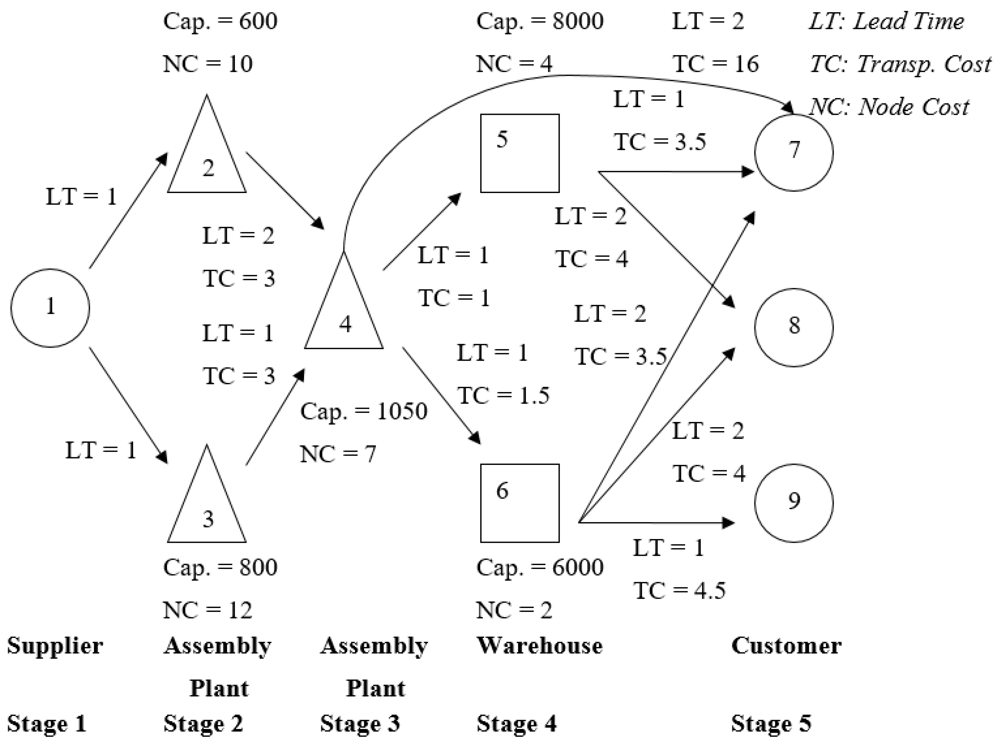
3. Illustrative Example

The business case for such systems is seen in the electronics and aviation industries, where queuing effects are experienced due to variations in processing times. For example, in the electronic industry, semiconductor wafers undergo reentrant process steps through several workstations, effectively creating a queuing network. In the aviation industry, machining can be quite intricate and varies every time a component is made, making the processing time non-deterministic. In addition, in the defense aviation industry, assembly time is non-deterministic because it is not only complex, but also involves extensive testing.

Consider a simple internal supply chain network with three assembly plants, two warehouses, one upstream supplier, and three downstream customers (Figure 1). Material flow starts from suppliers, undergoes transformation and finally reaches customers. NC, TC, and LT are abbreviations for the node cost, transportation cost, and lead time, respectively. Note that direct shipping is allowed between assembly node 4 in stage 3 and customer node 7 in stage 5, with a higher transportation cost. Node 7 is supplied by nodes 4, 5, and 6, and node 8 is supplied by nodes 5 and 6. Node 9 is supplied only by node 6. We assume that the supplier’s supplier charges a constant price for raw materials.

The bill of materials is shown in Figure 2.

Table 1. Unit holding costs per time period (4% of unit cost).

Item ID	1	2	3	4	5	6	7	8
Unit Cost	4	10	18	5	3	2	15	200
Unit Holding Cost	0.016	0.04	0.072	0.02	0.012	0.08	0.06	0.8

,

Table 2. Capacity consumed per time period by a unit in trans-shipment nodes.

Node ID	Item ID	Capacity Consumed by Unit
2	8	8
3	8	8

,

Table 3. Capacity consumed per time period by a production run in production nodes.

Node ID	Recipe ID	Capacity Consumed by Production
4	1	1
4	2	2
5	1	1
5	2	2
6	3	3

and

Table 4. Product-dependent unit cost in all intermediate nodes per time period.

Node ID	Item ID	Product Dependent Unit Cost
2	8	2
3	8	2.2
4	1	0.645
4	2	0.8
4	3	0.965
4	4	1.025
4	5	1.14
4	6	1.26
4	7	1.45
5	1	0.77
5	2	0.925
5	3	1.09
5	4	1.15
5	5	1.265
5	6	1.385
5	7	1.575
6	3	1.215
6	7	1.7
6	8	2.75

show the parameter settings. Raw material (items 1 to 6) are purchased by the firm from a supplier in stage 1. They then enter assembly nodes 2 or 3, where two recipes are used. Sub-final items 3 and 7 leave stage 2 and enter assembly node 4 for final production. End product 8 goes through either warehouse 5 or 6 in stage 4 to reach the customers in the final stage. We also set an upper bound on space requirements at assembly nodes of 600 and 300 units for input items and for output items, respectively. The length of each time period is one week.

The scenarios below show how the model can be used for demand planning. In all the scenarios below, the value of β in DPP was assumed to be 0. All problems below were run on a Pentium III Personal Computer with a Celeron CPU running at 850 MHZ using MINOS 5.5. The problems ran in less than a few seconds. The objective function values below are in the same units (dollars, Euros, yen, etc.) as the unit, unit holding, and transportation costs.

3.1. Base-Case Scenario: Quoting Due Dates to Customers

It is assumed that initial inventories are 200 units in IT nodes, and 100 units and 50 units in IP nodes for input and output products, respectively.

Table 5. RFQ for all customers in basic scenario.

Node/Time Period/Demand	6	7	8	9	10	11	12
Node 7	80	75	120	135	170	140	100
Node 8	30	45	50	45	55	40	35
Node 9	50	150	20	100	20	25	60
Total Demand	160	270	190	280	255	205	195

shows the RFQ data at customer nodes 7, 8, and 9 for time periods 6 to 12. Let us assume that none of this demand is committed, that is, all demand values are treated as new demand or RFQ with assumed lateness cost on new demand.

Solving DPP, the optimal objective function value obtained is 227,204.74, showing that all deliveries can be made within 12 time periods. However, this does not mean every delivery can be made in time. Scenario 1 (base case) in

Table 6. Lateness in various scenarios.

Scenario	Node ID	Time Period	Total Lateness
Scenario 1: Base Case	7	10	123.34
	8	10	25
	9	9	23.34
	9	10	20
	Objective Function Value = 227,204.74
Scenario 2: Increased Demand for Customer 8	7	10	193.34
	8	10	25
	9	9	93.34
	9	10	20
	Objective Function Value = 278,427.98
Scenario 3: New Recipe	7	10	131.9
	7	11	17.17
	9	9	36.67
	9	10	31.67
	Objective Function Value = 257,674.85
Scenario 4: Order Cancellation	7	11	6.67
	9	11	6.67
	Objective Function Value = 159,620.03

shows the total amount of lateness to customers 7, 8, and 9. The lateness values in the table should be used by the firm to promise orders.

3.2. Order Change: Increased Demand for Customer 8

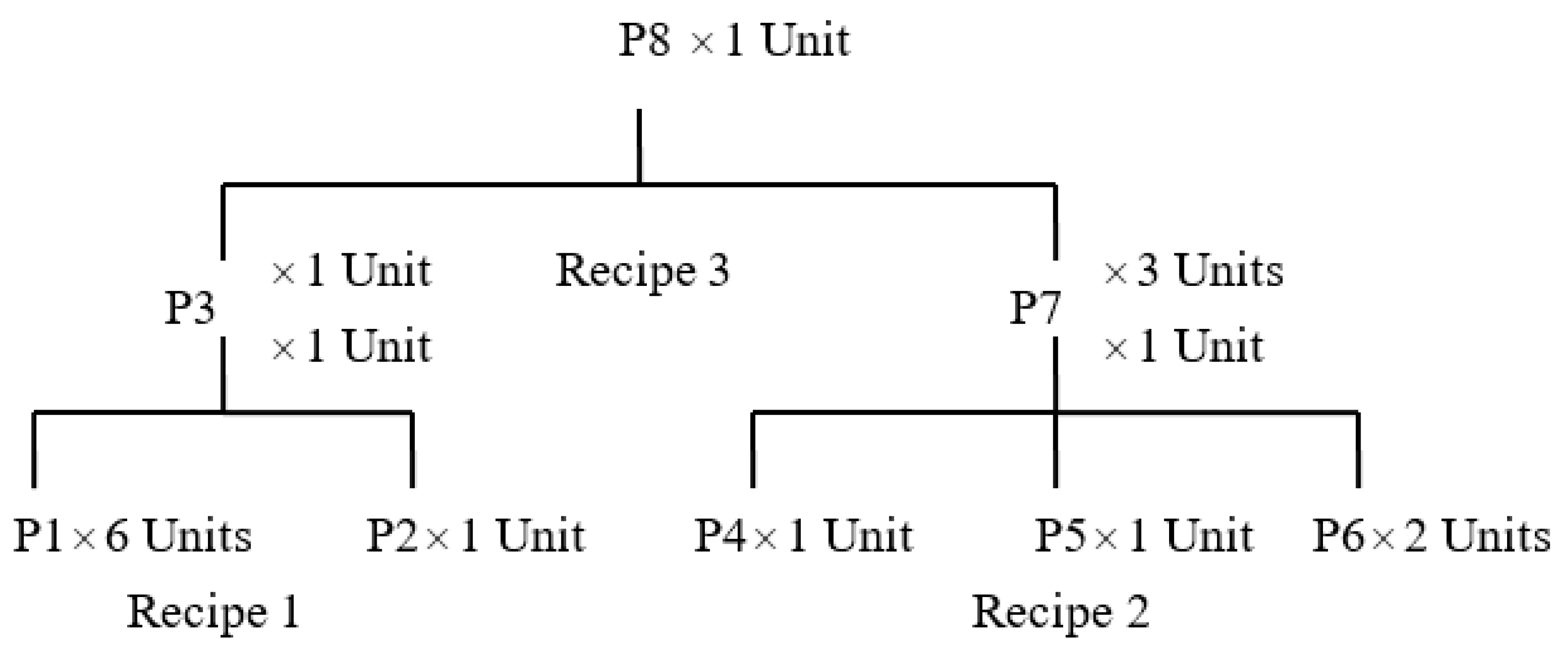
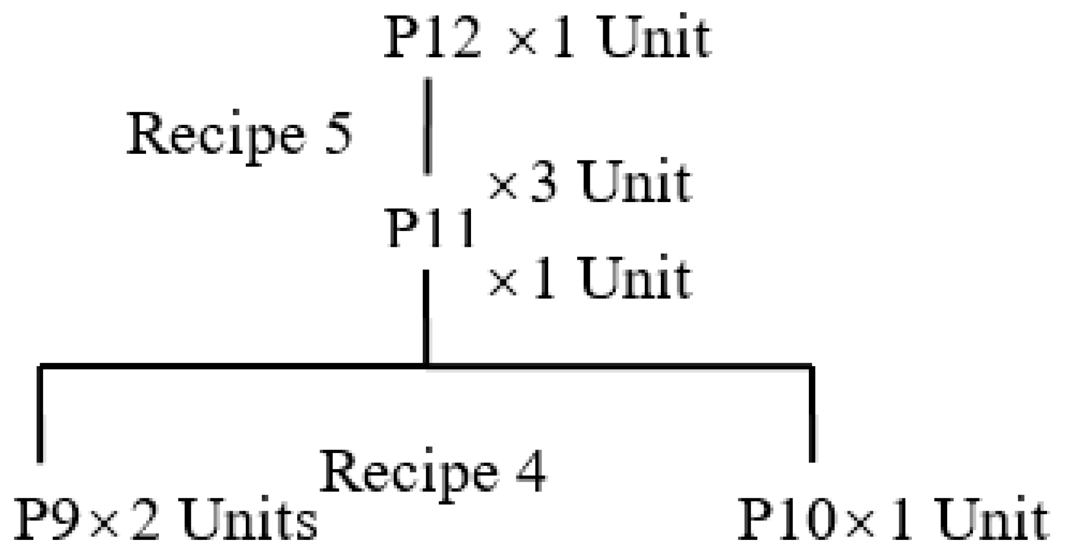
Assume that customer 8 increases demand from time period 10 from 55 units to 90 units even before the firm has had a chance to respond to the RFQ in Table 6. By the running the model again, it is seen that this change causes increase in lateness for customers 7 and 9, and the optimal objective function value is 278,427.98 (see Scenario 2 in Table 6). The increase in objective function value includes two types of cost: the cost to push more product through the system and the cost of late deliveries at customers 7 and 9, beyond the lateness they agreed to. Clearly, the firm should charge customer 8 at least the difference in cost (278,427.98 − 227,204.74 = 51,223.24) in order to accept the increase.

3.3. New Recipe

Assume that the customer at node 8 comes in with an RFQ for a second item that has a new bill of material (Figure 3) in addition to the older RFQ for item 8, all before the firm has responded to any RFQ. The new final item 12 is assumed to have higher RFQ lateness cost than item 8. The customer asks for an additional 25 and 15 units of item 12 at time periods 11 and 12, respectively.

After solving DPP, the result shows that this scenario causes even more lateness for the other two customers. The optimal objective function value is 257674.85 (Scenario 3 in Table 6). Thus, the firm should charge the customer at least the difference in cost (257,674.85 − 227,204.74 = 30,470.11) to accept this change to the RFQ.

3.4. Order Cancellation

Going back to the basic scenario, it is assumed that the RFQs are accepted. Subsequently, customer at node 8 cancels his or her order in time period 10. DPP is solved again to evaluate the consequence of this cancellation. The optimal objective function value drops to 159,620.03 (Scenario 4 in Table 6), and lateness for the other two customers is greatly improved. Only customers 7 and 9 will have late deliveries; in each case, 6.67 units of demand in time period 11 will be delayed by 1 period.

3.5. Demand Planning and Capacity Bottleneck Alleviation

Another feature of this model is its ability to identify the resource bottlenecks of each time period dynamically. The goal is minimizing total cost, instead of lateness. Four decision factors determine how to alleviate a bottleneck: dual price, sensitivity, cost of adding one unit of capacity, and the ceiling on how much capacity can be added. At any given point in time, the resource with the highest positive value after subtracting the corresponding cost of adding a unit of capacity from its dual price is regarded as the bottleneck at that time period. The amount of capacity to be added is decided by the sensitivity range and the ceiling. Demand managers can find and remove core bottlenecks using the algorithm described below:

Bottleneck Alleviation Algorithm

Step 1: Solve the model DPP and obtain resource dual prices and sensitivity ranges.

Step 2: Find the resource with the highest value after subtracting the corresponding cost of adding capacity from its dual price. If the value is positive, go to step 3; otherwise, stop.

Step 3: Add capacity up to the ceiling or upper bound determined by the sensitivity range of the bottleneck.

Step 4: Go to step 1.

The procedure thus alleviates bottlenecks by solving the model repeatedly after capacity modifications. Consider the base scenario and the effects of adding overtime capacity, which cannot exceed 15% of the regular capacity for all production. Assume that the cost of adding one unit of capacity is 100 for node 4 and 130 for node 5. After DPP is solved, the dual prices on the capacity constraint are as specified in Run 1 of

Table 7. A Summary of four runs of the bottleneck alleviation algorithm.

Node ID	Time Period	Capacity Cost	RUN #1				RUN #2
			Capacity	Dual Price	Improvement	Sensitivity Range (Upper Bound)	Capacity	Dual Price	Improvement	Sensitivity Range (Upper Bound)
4	2	100	600	165.88	1025.09	615.56	600	165.9	1025.4	615.56
4	3	100	600	123.03	537.29	623.33	600	123.04	537.52	623.33
4	4	100	600	80.17	−462.63	623.33	600	80.18	−462.4	623.33
4	5	100	600	37.31	−1462.6	623.33	600	37.32	−1462.3	623.33
4	6	100	600	1	−26,070	863.33	600	1	−26,070	863.33
5	2	130	800	186.32	1313.95	823.33	823	186.33	18.5889	823.33
5	3	130	800	164.87	542.577	815.56	800	164.89	7.6758	800.22
3	4	130	800	121.98	−187.11	823.33	800	121.98	−2.6466	800.33
5	5	130	800	79.16	−1186.1	823.33	800	79.17	−16.774	800.33
5	6	130	800	36.26	−2187	823.33	800	36.27	−30.931	800.33
Node ID	Time Period	Capacity Cost	RUN #3				RUN #4
			Capacity	Dual Price	Improvement	Sensitivity Range (Upper Bound)	Capacity	Dual Price	Improvement	Sensitivity Range (Upper Bound)
4	2	100	615	165.9	6172.85	708.67	690	165.9	1230.35	708.67
4	3	100	600	123	1400.47	660.89	600	123	429.41	618.67
4	4	100	600	80.18	−1856.5	693.67	600	80.18	−370.04	618.67
4	5	100	600	37.33	−5870.3	693.67	600	37.33	−1170	618.67
4	6	100	600	1	−18546	787.33	600	1	−3695.7	637.33
5	2	130	823	186.33	2057.17	859.52	823	186.33	1051.68	841.67
5	3	130	800	164.89	3268.15	893.67	800	164.89	651.396	818.67
3	4	130	800	121.98	−751.23	893.67	800	121.98	−149.73	818.67
5	5	130	800	79.17	−4761.2	893.67	800	79.17	−949	818.67
5	6	130	800	36.27	−8779.7	893.67	800	36.27	−1166	812.44

.

It is clear that node 5 at time period 2 is the bottleneck. Twenty-three extra capacity units are added to the bottleneck (this is less than 15% of the basic capacity), based on the sensitivity range (823.33–800), and the model is run again. The optimal objective function value is 225,907.56 (see Run 2 of Table 7). The total lateness for all nodes drops to 178.52, and node 4 at time period 2 becomes the new bottleneck. In run 3, the problem is solved again with 615 units of capacity in node 4, time period 2, because the sensitivity range indicates that the capacity can be increased up to 615.56 units. After this run, the optimal objective function value is 221,929.13, and the total lateness across all nodes is 171. Node 4 at time period 2 is still the bottleneck (run 3 of Table 7). Although increasing capacity up to 708.67 is the best solution, only 75 more capacity units can be added to the bottleneck because of the 15% ceiling rule. In the last run shown in Table 7, the optimal objective function value decreases to 212,500.85 (decreased by 4.24% from the third run), and the total lateness for all nodes is 133.51 (decreased by 21.92% from the third run). The bottleneck moves back to node 5 at time period 2. The process of bottleneck elimination can be continued in this fashion until it is not economical to alleviate the bottleneck.

4. Modelling Congestion Effects

In this section, we extend the model developed in Section 2 to incorporate congestion effects.

4.1. Clearing Functions

The throughput of a network node (output in a time period) depends on both the nominal capacity of the node and the WIP of input product available, the former being the upper bound on throughput. Without any congestion in the system, the clearing function is linear (function 1 in Figure 4). Note that function 1 is implicit in the DPP model described in Section 2 and is defined by Constraints (7) and (10). However, when there is congestion in the system, the WIP versus throughput relationship is more like function 2 shown in Figure 4. Karmarkar [18] and Srinivasan et al. [17] introduced the concept of the concave nonlinear capacity function to link WIP and lead time in capacity planning for discrete time period models by developing clearing functions based on queuing models. The concavity assumption is appropriate for most production facilities, where production rate increases asymptotically to a limit as the WIP level increases. Karmarkar [18] developed clearing function formulations for a single commodity model in an M/M/1 queuing system, and a multi-commodity model in an M/G/1 queuing system, using continuous time periods. An analogous clearing function for a single-product discrete time period model based on input/output control was also discussed. Conway et al. [35] found that the shape of the capacity versus WIP curve was sharply concave for serial production lines. Bhatnagar et al. [36] also observed the concavity of the clearing function in assembly systems using a simulation approach.

4.2. The Nonlinear Clearing Function Model

A new continuous variable, Z_t,j,r ($\ge 0$), is introduced to model capacity congestion:

Zt,j,r

maximum number of production runs made using recipe r $\in$ Rj at node j $\in$ IP in time period t.

The clearing function illustrations in Figure 4 involve only one product. When several products are involved, the input item that constrains the maximum number of production runs in time period t for a recipe represents the critical WIP for that time period. Therefore, the following constraint set is added to the formulation:

$$Z_{t,j,r}\le \frac{x_{t,j}^m}{R{I}_{j,r}^m} \forall j\in IP,\forall t,\forall r\in R_j,\forall m\in IP{T}_{j,r}$$

(22)

$$Z_{t,j,r}\ge 0 \forall j\in IP,\forall t,\forall r\in R_j$$

(23)

The ratio on the right-hand side of (22) represents the number of runs of recipe r at node (t,j) that can be made based on initial inventory of input product m. Since a recipe has many input products, the available (maximum) number of production runs is constrained by the product for which this ratio is the smallest.

The clearing functions described in this paper so far are based on the single-product queue. In order to operationalize these clearing functions, we have to ensure that only one product is produced at a resource at a given time. We first examine the case when only one recipe can be run at a node in a given time period. In this case, the actual number of production runs that can be made at a production node depends on the nominal capacity of the node C_t,j, the capacity usage V_j,r, and the clearing function, defined as $g_{j,r}(Z_{t,j,r})$, and is modelled by Constraint (24). Constraint (7) of the formulation is now redundant (since we will show in the next section the value of the clearing function $g_{j,r}(Z_{t,j,r})$ approaches 1 as $Z_{t,j,r}$ approaches infinity), ensures that the sum of the production usage of all recipes at a node does not exceed its nominal capacity. In order to ensure that only one recipe can be run at a time during a given time period, we introduce a new zero/one variable, Y_t,j,r, which takes a value of 1 if recipe r is run at node (t,j). In Constraint (25), M is a large number, and therefore, the binary variable Y_t,j,r is set to 1 when N_t,j,r is non-zero. Constraint (26) enforces the one-recipe at a node-time rule. Constraint (27) simply defines the Y_t,j,r’s as binary variables.

$$N_{t,j,r}\le \frac{C_{tj}}{V_{j,r}}{g}_{j,r}(Z_{t,j,r}) \forall j\in IP,\forall t,\forall r\in R_j$$

(24)

$$Y_{t,j,r}\ge \frac{N_{t,j,r}}{M} \forall j\in IP,\forall t,\forall r\in R_j$$

(25)

$${\displaystyle \sum _{r\in R_j}{Y}_{j,r}}\le 1 \forall j\in IP,\forall t$$

(26)

$$Y_{t,j,r}\in \{0,1\} \forall j\in IP,\forall t,\forall r\in R_j$$

(27)

The non-linear extension of DPP may now be written as:

DPPNL: Minimize (1)

Subject to: (2) to (6), (8) to (16) and (22) to (27)

It must be noted that both $g_{j,r}(Z_{t,j,r})$ and N_t,_j,r are defined as continuous variables, while in reality, they should both be integers. This may not be an unreasonable assumption in the rolling-horizon planning context, where only the decisions in period one are implemented and all the decisions in subsequent periods are re-planned. Therefore, a simple rounding down of these variable values, while not optimal for discrete parts assembly processes, would be feasible and practical.

As mentioned before, a big difference between the approach in the literature and this work is that instead of working directly with products, the recipes are the virtual entities queueing at the nodes. This is an important contribution of this paper, because we model congestion in assembly or blending through recipes.

In order to allow several recipes to be run at a node in the same time period, we can modify Constraint (24) in a manner analogous to the capacity constraints in Asmundsson et al. [23]. The capacity for each recipe r is partitioned through Constraint (28), separable by recipes as follows:

$$N_{t,j,r}\le {\alpha }_{t,j,r}\frac{C_{tj}}{V_j}{g}_j({\displaystyle \sum _{r\in R_j}{Z}_{t,j,r}}) \forall j\in IP,\forall t$$

(28)

$${\displaystyle \sum _{r\in R_j}{\alpha }_{t,j,r}}=1 \forall j\in IP,\forall t$$

(29)

This method uses a partitioning variable, α_tjr, for each recipe r as a multiplier in the right-hand side of Constraint (28), with the additional condition that the sum of the α_tjr’s is 1, as shown in Constraint (29). Constraints (25) to (27) may be dropped for this case. Also, the variable V_j is used instead of variable V_j,r, because the average capacity used by one production run of recipe r is now defined in terms of the node and is an average across all recipes at the node.

In what follows, three different clearing functions are adapted from the literature to our model. We will show that they are concave and continuously differentiable, making them computationally tractable (Asmundsson et al. [23] assume that the clearing function for the partitioned capacity case in Constraint (28) is concave). The assumption behind the clearing functions above, which are all separable by recipe r, is that during a period t, one recipe is run repeatedly for steady-state queues to form. In other words, it is assumed that different recipe runs are not mixed together because the queuing behaviour of a multi-class node is different from the queuing behaviour of a single-class node.

4.2.1. Input/Output Clearing Function

Karmarkar [18] employs the following function based on the M/M/1 queue:

$${X_t}_{ }= \mathit{Min} [P\frac{W_{t-1}+R_t}{W_{t-1}+R_t+k}, W_{t-1}+ R_t]$$

where W_t-1 is the initial WIP in time period t, R_t the constant release rate in time period t, X_t the actual production rate in time period t, and P the maximum production possible in time period t. The constant k (>0) is used to generate a family of clearing functions. The second argument of the above function is that production cannot also exceed the total of WIP in the previous period and the current release. In our model, Constraint (22) ensures this. Also, $\frac{C_{t,j}}{V_{j,r}}$ is the maximum production rate per time period at node (j,t), using recipe r, with Z_t,j,r representing the available (maximum) number of runs, and N_t,j,r being the actual number of runs. Hence, the analogous form of the constraint corresponding to the input/output clearing function of Karmarkar [18] is as follows:

$$N_{t,j,r}\le \frac{C_{t,j}}{V_{j,r}}\frac{Z_{t,j,r}}{Z_{t,j,r}+k} \forall j\in IP,\forall t,\forall r\in R_j$$

(30)

$$\mathrm{Clearly}, \underset{Z_{t,j,r}\to \infty }{\lim }\frac{Z_{t,j,r}}{Z_{t,j,r}+k}=1$$

Strictly speaking, this constraint models the clearing function for a single server station. However, since DPPNL is a supply chain network model, constraint may be appropriate where a bottleneck M/M/1 workstation is identified. Alternatively, individual M/M/1 workstations could be modelled in the supply chain network (the model size will then be large).

4.2.2. M/D/1 Clearing Function

This function is adapted from Karmarkar et al. [15], who use an M/G/1 model to study lead time and WIP as a function of batching policy for multiple products. Consider the set IP as an open queuing network where each node is a workstation. Also, assume that there is only one recipe per production node. Since each run represents the processing of a group of components (from the input components set), and assuming that the assembly will not proceed until there is at least one group of components available,

${\rho }_{j,r}$ = I sever utilization per time period at node j using recipe r.

T_q = average time spent in queue.

Note that batch sizes are considered to be one, and variations in processing time are ignored (since the M/D/1 assumes constant service time).

$${\rho }_{j,r}= \frac{N_{t,j,r}}{\frac{C_{t,j}}{V_{j,r}}}=\frac{N_{t,j,r}}{\kappa } (\mathrm{Where}, \kappa =\frac{C_{t,j}}{V_{j,r}})$$

Using the Pollaczek–Khintchine formula for the M/D/1 queue:

$${T_q}_{ }= \frac{{\rho }_{j,r}{}^2}{2(1-{\rho }_{j,r})}\frac{1}{{\lambda }_{j,r}}=\frac{{(\frac{N_{t,j,r}}{\kappa })}^2}{2(1-\frac{N_{t,j,r}}{\kappa })}\frac{1}{N_{t,j,r}}=\frac{N_{t,j,r}}{2\kappa (\kappa -N_{t,j,r})}$$

Applying Little’s law (Hopp and Spearman [37]):

$$Z_{t,j,r} = N_{t,j,r}(T_q+\frac{1}{\kappa }) = N_{t,j,r}(\frac{N_{t,j,r}}{2\kappa (\kappa -N_{t,j,r})}+\frac{1}{\kappa })=\frac{2\kappa N_{t,j,r}-N_{t,j,r}^2}{2\kappa (\kappa -N_{t,j,r})}$$

Solving for N_t,j,r gives:

$$N_{t,j,r}=\kappa (Z_{t,j,r}+1-\sqrt{Z_{t,j,r}^2+1})=\frac{C_{t,j}}{V_{j,r}}(Z_{t,j,r}+1-\sqrt{Z_{t,j,r}^2+1})$$

To use the same functional form as in Constraint (24), the above equation is rewritten as:

$$N_{t,j,r}\le \frac{C_{t,j}}{V_{j,r}}(Z_{t,j,r}+1-\sqrt{Z_{t,j,r}{}^2+1}) \forall j\in IP,\forall t,\forall r\in R$$

(31)

Again,

$$\underset{Z_{t,j,r}\to \infty }{\lim }(Z_{t,j,r}+1-\sqrt{Z_{t,j,r}{}^2+1})=1$$

This clearing function representation is applicable for an M/D/1 bottleneck station at an aggregate node in the supply chain network. Alternatively, the workstations in the queuing network can be represented as individual nodes in the network.

4.2.3. General Clearing Function

This function is adapted from Srinivasan et al. [17], and is modelled as follows:

$$g_{j,r}(Z_{t,j,r})=1-e^{-\mu Z_{t,j,r}},$$

where $\mu$ can be assigned any value to generate a family of clearing functions. Setting μ= $\frac{V_{j,r}}{C_{t,j}}$ results in the value of the function being always below the 45-degree line. To use the same functional form as in Constraint (24), the congestion constraint is written as:

$$N_{t,j,r} \le \frac{C_{t,j}}{V_{j,r}}(1-e^{-\mu Z_{t,j,r}})$$

(32)

As before,

$$\underset{Z_{t,j,r}\to \infty }{\lim }(1-e^{-\mu Z_{t,j,r}})=1$$

This clearing function is generic and useful when the queuing behaviour at a node is complex and the underlying process is not understood. However, there may empirical data to fit the clearing function using regression to choose the value of the parameter µ.

The function $g_{j,r}(Z_{t,j,r})$ is concave in all three cases. A question that arises is which of these functions should be used. The assumptions behind the first two clearing functions (Section 4.2.1 and Section 4.2.2) should be looked at carefully before applying either. In the case of the general clearing function (Section 4.2.3), it can be used almost universally. In any case, the parameters chosen should reflect the throughput characteristics of the production system.

DPPNL has a linear objective function with linear constraints and a non-linear constraint, either Constraint (30), Constraint (31) or Constraint (32). Therefore, DPPNL can be solved numerically using a nonlinear programming package such as MINOS, which uses the projected augmented Lagrangian method of Robinson [38]. The next section shows how two linear programming-based algorithms can be used to solve the model.

4.3. Algorithms for DPPNL

Two different algorithms are proposed for DPPNL: inner approximation using piecewise linear programming and outer approximation using the Kelley’s cutting plane method.

4.3.1. Inner Approximation

The clearing function $g_{j,r}(Z_{t,j,r})$ can be represented as a summation of continuous single-variable piecewise linear functions to give an inner approximation. One of the most important issues in piecewise linear programming is whether the adjacency criterion will hold. Fortunately, the adjacency criterion is automatically satisfied by the optimal solution in a convex separable program under which our problem is a subset (Simmons [39]). Thus, no binary variables are necessary to explicitly model adjacencies.

To implement the piecewise linear approximation, I pieces (I + 1 points) are used for each Z_t,j,r. Herein, νⁱ_j,r is defined as the coordinate of each piece variable, and ${\lambda }_{t,j,r}^i$ as the new decision variable in the piecewise linearized function. The concave function is evaluated at each point g_j,r(νⁱ_j,r).

Since $g_{j,r}(Z_{t,j,r})={\displaystyle \sum _{i=0}^I{g}_{j,r}({\nu }_{j,r}^i){\lambda }_{t,j,r}^i}\forall j\in IP,\forall t,\forall r\in R_j$, g_j,r(Z_t,j,r) is replaced with the piecewise linearized summation ${\displaystyle \sum _{i=0}^I{g}_{j,r}({\nu }_{j,r}^i){\lambda }_{t,j,r}^i}$ and Constraints (33), (34), and (35) are introduced, as shown below:

$${\displaystyle \sum _{i=0}^I{\lambda }_{t,j,r}^i=1} \forall j\in IP,\forall t,\forall r\in R_j$$

(33)

$$Z_{t,j,r}={\displaystyle \sum _{i=0}^I{\nu }_{j,r}^i{\lambda }_{t,j,r}^i} \forall j\in IP,\forall t,\forall r\in R_j$$

(34)

$$0\le {\lambda }_{t,j,r}^i\le 1 \forall j\in IP,\forall t,\forall r\in R_j$$

(35)

The optimal solution to DPPNL can be obtained to any degree of accuracy by increasing the number of pieces. However, the formulation is entirely linear and can be solved efficiently.

4.3.2. Outer Approximation

Unlike the inner approximation method that solves one large DPPNL problem, the Kelley’s cutting plane algorithm (KCP) may be used as an outer approximation technique. Outer approximation requires several iterations, as the problem size grows slowly with each iteration. A concave polyhedron is formed, iteration by iteration, to cover the original smooth concave function. The problem is first solved with the nonlinear constraint replaced by linear constraints, which are above the corresponding concave constraints and thus provide a feasible region larger than what is allowable. Constraints are generated by adding additional tangential lines to the concave function, based on the previous solution, at the point where the solution is infeasible for the original problem. The problem is solved again until the stopping condition is met; the solution should be feasible or the decrease in optimal objective function value must be less than the scalar $\epsilon$. The cutting plane method thus develops an outer approximation. An optimal or near optimal solution can be reached by choosing an appropriate scalar, and the number of iterations can increase if more accuracy is desired.

The outer approximation (Kelley’s cutting plane) algorithm for DPPNL is as follows:

Step 1: Initialization

(1)

Set iteration counter i = 0, $L=\varnothing$.

(2)

Drop Constraint (24) and define the following linear constraint:

$$N_{t,j,r}\le \frac{C_{tj}}{V_{j,r}}(a_{t,j,r}^0+b_{t,j,r}^0{Z}_{t,j,r}) \forall j\in \left\{IP\right\},\forall t,\forall r\in R_j(L^0)$$

where:

$$b_{t,j,r}^0=\nabla g_{j,r}(0),a_{t,j,r}^0=0$$

Choose a scalar $\epsilon$.

Step 2: Main step

(1)

Set $L\leftarrow L\cup L^{\mathrm{i}}$.

(2)

Solve DPPNL.

Let $N_{t,j,r}^i,Z_{t,j,r}^i$ denote the solution to iteration i.

Let $O^i$ be the optimal objective function value to iteration i.

Is $g_{j,r}(Z_{t,j,r}^i)-(a_{t,j,r}^i+b_{t,j,r}^i{Z}_{t,j,r}^i)<0$ and $O^{i-1}-O^i>\epsilon$?

If no: stop; the optimal solution has been found.

If yes: I = i + 1

Write new constraint:

$$N_{t,j,r}\le \frac{C_{tj}}{V_{j,r}}(a_{t,j,r}^i+b_{t,j,r}^i{Z}_{t,j,r})\forall j\in IP,\forall t,\forall r\in R_j(L^i)$$

where:

$$b_{t,j,r}^i=\nabla g_{j,r}(Z_{t,j,r}^{i-1}),a_{t,j,r}^i=g_{j,r}(Z_{t,j,r}^{i-1})-b_{t,j,r}^i{Z}_{t,j,r}^{i-1}$$

Go to step 2

If no: stop.

Convergence is guaranteed when a feasible solution exists and the nonlinear constraints are convex and continuously differentiable (Zangwill [40], Luenberger and Ye [41], pp. 463–465).

Proposition 1.

The I/O clearing function in Section 4.2.1 is concave and continuously differentiable.

$$g_{j,r}(Z_{t,j,r})=\frac{C_{t,j}}{V_{j,r}}\frac{Z_{t,j,r}}{Z_{t,j,r}+\kappa }$$

Taking the first derivative, $g_{j,r}{}^{\prime }(Z_{t,j,r})=\frac{C_{t,j}}{V_{j,r}}\frac{\kappa }{{(Z_{t,j,r}+\kappa )}^2}$, it can be seen that $g_{j,r}(Z_{t,j,r})$ is continuously differentiable in the domain $Z_{t,j,r}\ge 0$ (since k > 0).

The second derivative, $g_{j,r}{}^{″}(Z_{t,j,r})=\frac{-2C_{t,j}\kappa }{V_{j,r}}/{(Z_{t,j,r}+\kappa )}^3$, is always negative. Therefore, $g_{j,r}(Z_{t,j,r})$ is concave.

Proposition 2.

The M/D/1 clearing function in Section 4.2.2 is concave and continuously differentiable.

$$g_{j,r}(Z_{t,j,r})=\frac{C_{t,j}}{V_{j,r}}(Z_{t,j,r}+1-\sqrt{Z_{t,j,r}{}^2+1})$$

Taking the first derivative, $g_{j,r}{}^{\prime }(Z_{t,j,r})=\frac{C_{t,j}}{V_{j,r}}(1-1/\sqrt{Z_{t,j,r}{}^2+1})$, it can be seen that $g_{j,r}(Z_{t,j,r})$ is continuously differentiable in the domain $Z_{t,j,r}\ge 0$.

The second derivative, $g_{j,r}{}^{″}(Z_{t,j,r})=\frac{-C_{t,j}}{V_{j,r}}/{(\sqrt{Z_{t,j,r}{}^2+1})}^{3/2}$, is always negative. Therefore, $g_{j,r}(Z_{t,j,r})$ is concave.

Proposition 3.

The general clearing function in Section 4.2.3 is concave and continuously differentiable.

$$g_{j,r}(Z_{t,j,r})=1-e^{-\mu Z_{t,j,r}}$$

Taking the first derivative, $g_{j,r}{}^{\prime }(Z_{t,j,r})=\mu e^{-\mu Z_{t,j,r}}$, it can be seen that $g_{j,r}(Z_{t,j,r})$ is continuously differentiable in the domain $Z_{t,j,r}\ge 0$. The second derivative, $g_{j,r}{}^{″}(Z_{t,j,r})=-{\mu }^2{e}^{-\mu Z_{t,j,r}}$, is always negative. Therefore, $g_{j,r}(Z_{t,j,r})$ is concave.

Proposition 4.

DPPNL converges to a limit solution using the Kelley’s cutting plane method when any of the clearing functions in Section 4.2.1, Section 4.2.2 and Section 4.2.3 is used in Constraint (16).

Note that (24) may be rewritten as follows:

$$N_{t,j,r}-\frac{C_{tj}}{V_{j,r}}{g}_{j,r}(Z_{t,j,r})\le 0 \forall j\in IP,\forall t,\forall r\in R_j$$

From Propositions 1, 2, and 3, $g_{j,r}(Z_{t,j,r})$ is concave and continuously differentiable in each of the three cases for the clearing function. Hence, the $-g_{j,r}(Z_{t,j,r})$’s are differentiable convex functions, and the entire constraint set in DPPNL is convex. Luenberger and Ye [41] (pp. 463–465) show that the Kelley’s cutting plane method converges to a limit solution for such a problem.

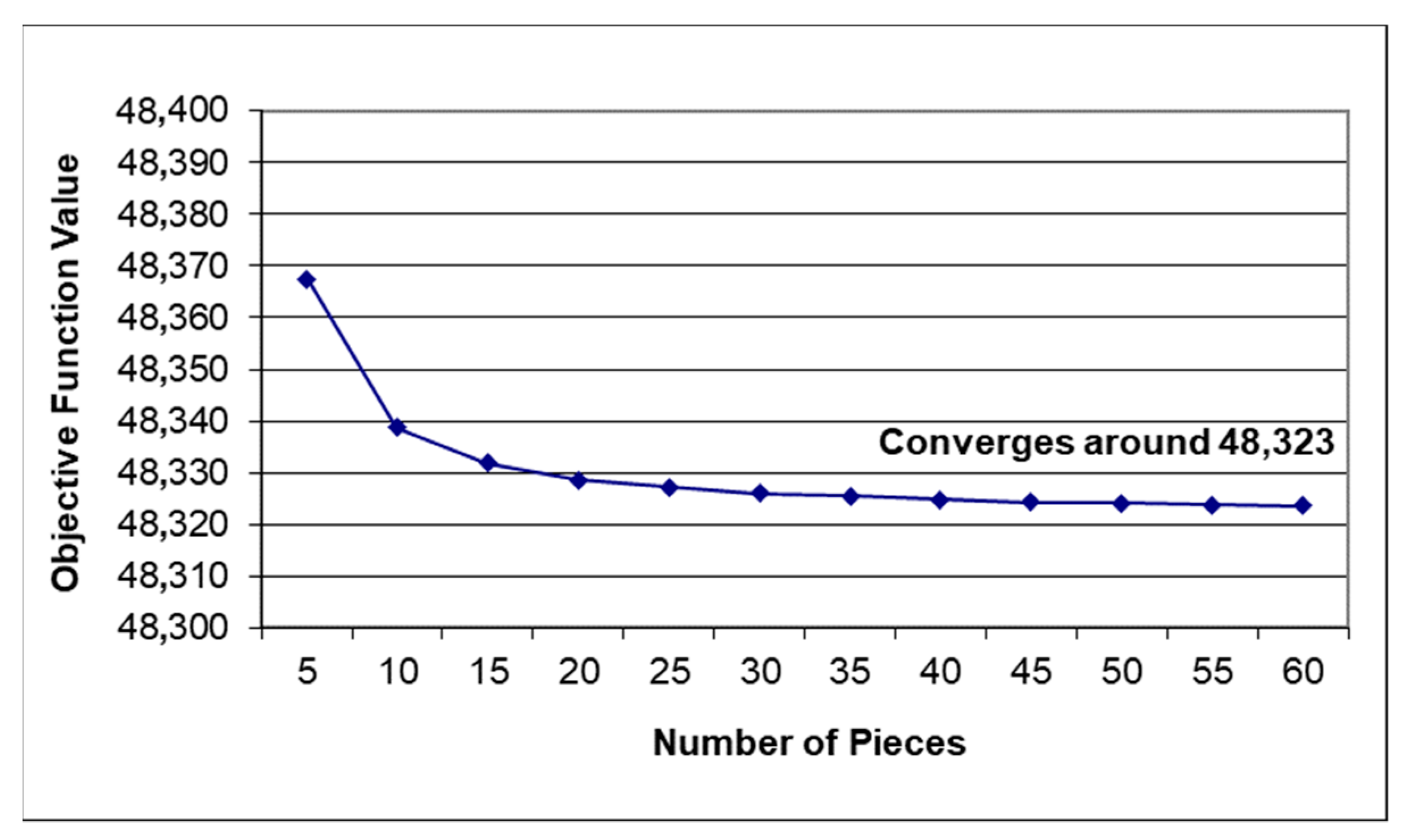
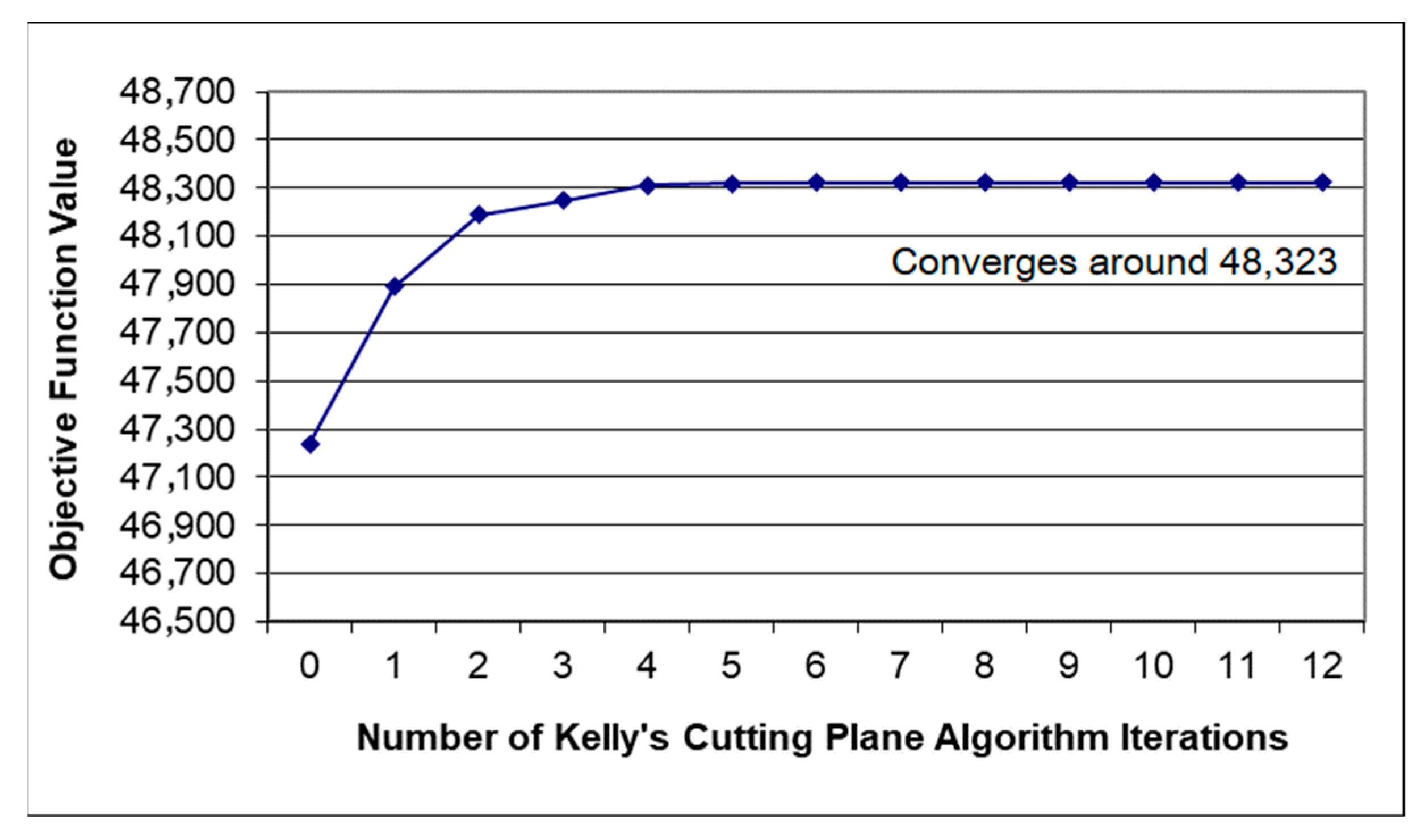
4.3.3. Computational Performance

In this section, results obtained by implementing the solution algorithms for DPPNL are discussed. All problems were run on a Pentium III Personal Computer with a Celeron CPU running at 850 MHZ.

Comparing Inner and Outer Approximation

For the sample case discussed in the paper, the RFQs in

Table 8. Demand data for DPPNL computations.

Node/Time Period/Demand	6	7	8	9	10	RFQ in Periods 11–18
Node 7	80	75	120	135	170	175
Node 8	30	45	50	45	55	44
Node 9	50	150	20	100	20	87
Total Demand	160	270	190	280	255	306

are used to solve the problem using inner approximation. The optimal solution converges to 48,323 when the number of pieces is 55. Figure 5 shows the results.

The same problem is solved using the outer approximation method. An objective function value of 48,323 is reached from the ninth iteration (cut) onwards, with no significant change. The results are shown in Figure 6.

As seen above, both methods converge to an objective function value of approximately 48,323. Outer approximation provides a more accurate result, but the gap between the starting value and the final value is quite large. On the other hand, inner approximation gives a less precise result, but the difference between the starting value and the final value is much smaller.

It is interesting to notice that outer approximation solves the fully relaxed problem at first and then tightens the constraint set as close to the nonlinear constraint as possible, iteration by iteration. In other words, the method always underestimates the real optimal objective function value. Inner approximation does exactly the opposite, i.e., it always overestimates the real optimal objective function value. Thus, the inner approximation result is the upper bound and the outer approximation result the lower bound on the optimal solution.

Model Solution Time for Different Problem Sizes

Different sizes of problems in the linear and nonlinear DPP without lateness models were tested to calibrate the model convergence and running time. A separate two-level bill of material with four items in the problems was added to get 12 commodities and two final items in the network. The production horizon for each problem class was 10 time periods. The general clearing function was used for the problem.

Table 9. DPPNL computation time.

Nodes	Time Periods	Total Number of Nodes	CPU Time (Seconds) for Outer Approximation **	CPU Time (Seconds) for Inner Approximation *	Percentage Increase (Inner Approximation Over Outer Approximation)
9	10	90	10.77	7.94	−26.40%
9	15	135	29.52	41.89	41.93%
12	10	120	23.51	27.69	17.76%
12	15	180	63.88	118.31	85.20%
15	10	150	32.68	38.34	17.33%
15	15	225	107.93	246.01	127.94%
18	10	180	71.96	132.3	83.86%
18	15	270	250.57	608.85	142.99%

* Based on 10pieces. ** Based on four Kelley’s cutting plane (KCP) cuts.

summarizes the run time results obtained using inner and outer approximation.

Outer approximation provides better performance than inner approximation in terms of CPU time as problem size increases, as can be seen in Table 9.

The augmented Lagrangian method implemented in MINOS 5.5 was used to evaluate the quality of the inner and outer approximation solutions. It may be seen in

Table 10. Objective function values obtained from augmented Lagrangian, inner approximation, and outer approximation.

Nodes	Time Periods	Augmented Lagrangian Optimal Obj. Fun. Value	Inner Approximation		Outer Approximation
			Optimal Obj. Fun. Value *	Gap (%)	Optimal Obj. Fun. Value **	Gap (%)
9	10	15,979.45	16,276.77	1.86	15,974.56	−0.031
9	15	13,861.32	13,903.68	0.31	13,855.34	−0.043
12	10	22,575.77	23,098.55	2.32	22,119.49	−2.02
12	15	18,867.84	18,918.27	0.27	18,843	−0.13
15	10	27,174.84	27,855.08	2.5	26,982.46	−0.71
15	15	23,914.94	23,925.25	0.04	23,833.54	−0.34

* Based on 10 pieces. ** Based on four KCP cuts. Time units in seconds.

that the solutions obtained by the approximations were reasonably close to the optimal objective function value obtained by the augmented Lagrangian method.

5. Conclusions

In this paper, we formulated a congestion model for of demand planning in supply chains that is general enough for the discrete-product or process industry. We illustrated the usefulness of the basic model in demand management via a series of scenarios in which the firm responds to RFQs, changes in demand, engineering changes, and due-date changes. The model’s use in capacity management was illustrated with an example. We extended the model to incorporate congestion effects using clearing functions that work at the recipe level, which is very general. The resulting model was nonlinear, and we developed and tested two linear programming-based algorithms to solve the nonlinear model. The performance of the two algorithms, one based on inner approximation and the other on outer approximation, was very good. This would allow for large-scale practical application of the model.

This research can be enhanced in many ways. One limitation of the model is that the number of recipes is a continuous variable, which is somewhat limiting for assembly systems. The queuing models considered are basic and assume that one recipe is run for a fairly long period of time for the queue to be stable. The concept of dual prices in Srinivasan et al. [17] and Kefeli and Uzsoy [27] can be applied in identifying not only capacity but also material bottlenecks. These limitations can be addressed in future research.

References

1. Beamon, B.M. Supply Chain Design and Analysis: Models and Methods. Int. J. Prod. Econ. 1998, 55, 281–294. [Google Scholar] [CrossRef]
2. Keskinocak, P.; Tayur, S. Quantitative Analysis for Internet-Enabled Supply Chains. Interfaces 2001, 31, 70–89. [Google Scholar] [CrossRef]
3. Askin, R.G.; Goldberg, J.B. Design and Analysis of Lean Poduction Systems; John Wiley and Sons: New York, NY, USA, 2002. [Google Scholar]
4. Billington, P.J.; McClain, J.O.; Thomas, L.J. Mathematical Programming Approaches to Capacity-Constrained MRP Systems: Review, Formulation and Problem Reduction. Manag. Sci. 1983, 29, 1126–1141. [Google Scholar] [CrossRef]
5. Baker, K.R. Requirement Planning. In Handbooks in Operations Research and Management Science. Logistics of Production and Inventory; Nemhauser, G.L., Rinnooy, K.A.H.G., Graves, S.C., Zipkin, P.H., Eds.; Elsevier Science Publishers B.V.: Amsterdam, The Netherlands, 1993; pp. 371–443. [Google Scholar]
6. Rota, K.; Thierry, C.; Bel, G. Capacity Constrained MRP System: A Mathematical Programming Model Integrating Forecasts Firm Orders and Suppliers; Departement d’Automatique, Universite Toulouse II Le Mirail: Toulouse, France, 1997. [Google Scholar]
7. Vidal, C.J.; Goetschaalckx, M. Strategic Production-distribution Models: A Critical Review with Emphasis on Global Supply Chain Models. Eur. J. Oper. Res. 1997, 98, 1–18. [Google Scholar] [CrossRef]
8. Arntzen, B.C.; Brown, G.G.; Harrison, T.P.; Trafton, L.L. Global Supply Chain Management at Digital Equipment Corporation. Interfaces 1995, 25, 69–93. [Google Scholar] [CrossRef] [Green Version]
9. Jang, Y.-J.; Jang, S.-Y.; Chang, B.-M.; Park, J. A combined model of network design and production/distribution planning for a supply network. Comput. Ind. Eng. 2002, 43, 263–281. [Google Scholar] [CrossRef]
10. Shapiro, J.F. Bottom-up vs. Top-down Approaches to Supply Chain Modeling. In Quantitative Models for Supply Chain Management; Tayur, S., Ganeshan, R., Magazine, M., Eds.; Kluwer Academic Publishers: Dordrecht, The Netherlands, 1999; pp. 737–759. [Google Scholar]
11. Rosenfield, D.B.; Shapiro, R.D.; Bohn, R.E. Implications of Cost-Service Trade-offs on Industry Logistics Structures. Interfaces 1985, 15, 47–59. [Google Scholar] [CrossRef]
12. Moodie, D.R.; Bobrowski, P.M. Due Date Demand Management: Negotiating the Trade-off Between Price and Delivery. Int. J. Prod. Res. 1999, 37, 997–1021. [Google Scholar] [CrossRef]
13. Venkatadri, U.; Srinivasan, A.; Montreuil, B. Demand and Price Planning in Supply Chain Networks. In Proceedings of the IERC 2003, Portland, OR, USA, 18–20 May 2003. [Google Scholar]
14. Upasani, A.; Uzsoy, R. Incorporating Manufacturing Lead Times in Joint Production-Marketing Models: A Review and Further Directions. Ann. Oper. Res. 2008, 161, 171–188. [Google Scholar]
15. Karmarkar, U.S.; Kekre, S.; Kekre, S. Lotsizing in Multi-Item Multi- Machine Job Shops. IIE Trans. 1985, 17, 290–298. [Google Scholar] [CrossRef]
16. Cohen, M.A.; Lee, H.L. Strategic Analysis of Integrated Production-Distribution Systems: Models and Methods. Oper. Res. 1988, 36, 216–228. [Google Scholar] [CrossRef]
17. Srinivasan, A.; Carey, M.; Morton, T.E. Resource Pricing and Aggregate Scheduling in Manufacturing Systems; Working paper; Purdue University: West Lafayette, IN, USA, 1989. [Google Scholar]
18. Karmarkar, U.S. Capacity Loading and Release Planning with Work-in-progress (WIP) and Leadtimes. Manuf. Serv. Oper. Manag. 1989, 2, 105–123. [Google Scholar]
19. Missbauer, H. Aggregate order release planning for time-varying demand. Int. J. Prod. Res. 2002, 40, 699–718. [Google Scholar] [CrossRef]
20. Asmundsson, J.; Rardin, R.; Uzsoy, R. Tractable Nonlinear Production Planning Models for Semiconductor Wafer Fabrication Facilities. IEEE Trans. Semicond. Manuf. 2006, 19, 95–111. [Google Scholar] [CrossRef]
21. Pahl, J.; Voß, S.; Woodruff, D.L. Production planning with load dependent lead times: An update of research. Ann. Oper. Res. 2007, 153, 297–345. [Google Scholar] [CrossRef]
22. Selcuk, B.; Fransoo, J.C.; De Kok, A.G. Work-in-process clearing in supply chain operations planning. IIE Trans. 2008, 40, 206–220. [Google Scholar] [CrossRef]
23. Asmundsson, J.; Rardin, R.L.; Turkseven, C.H.; Uzsoy, R. Production planning with resources subject to congestion. Nav. Res. Logist. 2009, 56, 142–157. [Google Scholar] [CrossRef]
24. Missbauer, H.; Uzsoy, R. Optimization Models of Production Planning Problems. In An Introduction to Computational Science; Springer Science and Business Media LLC: New York, NY, USA, 2010; pp. 437–507. [Google Scholar]
25. Kacar, N.B.; Monch, L.; Uzsoy, R. Planning Wafer Starts Using Nonlinear Clearing Functions: A Large-Scale Experiment. IEEE Trans. Semicond. Manuf. 2013, 26, 602–612. [Google Scholar] [CrossRef]
26. Charnsirisakskul, K.; Griffin, P.M.; Keskinocak, P. Order selection and scheduling with leadtime flexibility. IIE Trans. 2004, 36, 697–707. [Google Scholar] [CrossRef]
27. Kefeli, A.; Uzsoy, R. Identifying potential bottlenecks in production systems using dual prices from a mathematical programming model. Int. J. Prod. Res. 2015, 54, 2000–2018. [Google Scholar] [CrossRef]
28. Wang, S. Supply Chain Planning using Network Flow Optimization. Unpublished. Master’s Thesis, Department of Industrial Engineering, Dalhousie University, Halifax, Nova Scotia, 2003. [Google Scholar]
29. Chen, C.-Y.; Zhao, Z.-Y.; Ball, M.O. Quantity and Due Date Quoting Available to Promise. Inf. Syst. Front. 2001, 3, 477–488. [Google Scholar] [CrossRef]
30. Chen, C.-Y.; Zhao, Z.-Y.; Ball, M.O. A Model for Batch Advanced Available-to-Promise. Prod. Oper. Manag. 2002, 11, 424–440. [Google Scholar] [CrossRef]
31. Ball, M.O.; Chen, C.-Y.; Zhao, Z.-Y. Handbook of Supply Chain Analysis in the eBusiness Era; Simchi, L.D., David, W.S., Shen, M., Eds.; Kluwer Academic Publishers: Boston, MA, USA, 2004; pp. 447–484. [Google Scholar]
32. Shapiro, J.F.; Singhal, V.M.; Wagner, S.N. Optimizing the Value Chain. Interfaces 1993, 23, 102–117. [Google Scholar] [CrossRef]
33. Degbotse, A.; Denton, B.T.; Fordyce, K.; Milne, R.J.; Orzell, R.; Wang, C.-T. IBM Blends Heuristics and Optimization to Plan Its Semiconductor Supply Chain. Interfaces 2013, 43, 130–141. [Google Scholar] [CrossRef] [Green Version]
34. Fordyce, K.; Wang, C.-T.; Chang, C.-H.; Degbotse, A.; Denton, B.; Lyon, P.; Milne, R.J.; Orzell, R.; Rice, R.; Waite, J. The Ongoing Challenge: Creating an Enterprise-Wide Detailed Supply Chain Plan for Semiconductor and Package Operations. Int. Ser. Oper. Res. Manag. Sci. 2011, 152, 313–387. [Google Scholar]
35. Conway, R.; Maxwell, W.L.; McClain, J.O.; Thomas, L.J. The Role of Work-in-Process Inventory in Serial Production Lines. Oper. Res. 1988, 36, 229–241. [Google Scholar] [CrossRef]
36. Bhatnagar, R.; Chandra, P. Variability in assembly and competing systems: Effect on performance and recovery. IIE Trans. 1994, 26, 18–31. [Google Scholar] [CrossRef]
37. Hopp, W.J.; Spearman, M.L. Factory Physics: Foundations of Manufacturing Management, 2nd ed.; McGraw-Hill Irwin: New York, NY, USA, 2001. [Google Scholar]
38. Robinson, S.M. A quadratically-convergent algorithm for general nonlinear programming problems. Math. Program. 1972, 3, 145–156. [Google Scholar] [CrossRef]
39. Simmons, D.M. Nonlinear Programming for Operations Research. In International Series in Management; Prentice-Hall: Upper Saddle River, NJ, USA, 1975. [Google Scholar]
40. Zangwill, W.I. Nonlinear Programming: A Unified Approach; Prentice-Hall: Englewood Cliffs, NJ, USA, 1969. [Google Scholar]
41. Luenberger, D.G.; Ye, Y. Linear and Nonlinear Programming, 3rd ed.; International Series in Operations Research and Management Science ISOR 116; Hillier, F.S., Ed.; Springer: New York, NY, USA, 2008. [Google Scholar]
Figure 1. Example of a supply chain network.
Logistics 05 00003 g001
Figure 2. Bill of materials.
Logistics 05 00003 g002
Figure 3. Customer with new bill of material.
Logistics 05 00003 g003
Figure 4. Clearing function representation. WIP––work in progress.
Logistics 05 00003 g004
Figure 5. Inner approximation.
Logistics 05 00003 g005
Figure 6. Outer approximation.
Logistics 05 00003 g006