Bridging Accuracy and Interpretability: A Decision Support System for Stock Deployment and Additive Manufacturing Decisions in Spare Parts Distribution Networks

Abstract

Background: Spare parts distribution networks (DNs) play a strategic role in retailers’ profitability. Among DN configuration decisions, selecting the optimal stock deployment policy—centralised, decentralised, or hybrid inventory allocation across distribution centres (DCs)—critically affects service levels and logistics costs. This decision becomes more complex with additive manufacturing (AM) as an alternative to conventional manufacturing (CM). While AM enables production with shorter lead times, its higher costs alter stock deployment cost-effectiveness. Given the complexity of joint stock deployment and manufacturing decisions, retailers require decision support systems (DSSs). Methods: To address this need, we develop a DSS through a three-step methodology: (i) a mathematical model evaluates logistics costs across different stock deployment policies and manufacturing technologies; (ii) parametric analysis tests the model across 2000 realistic scenarios; (iii) Random Forest trained on this dataset predicts optimal solutions, with SHapley Additive exPlanations (SHAP) interpreting post hoc recommendations. Results: The DSS achieves 93.4% prediction accuracy—outperforming (+16.4%) the only comparable literature DSS (77%)—while explaining recommendations. SHAP reveals that AM and CM unit costs dominate decision-making, followed by backorder costs. Conclusions: Beyond individual spare parts recommendations, the DSS provides guidelines enabling retailers to maintain cost-effective DNs aligned with evolving customer needs and to plan valuable investments in AM.

1. Introduction

Over the past decade, intensifying market competition and shorter time-to-market expectations have elevated the strategic role of logistics in driving the profitability of spare parts distribution networks (DNs) [1]. In response, spare parts retailers have focused on improving logistics performance, with DN configuration optimisation emerging as a critical success factor [2]. A well-configured DN contributes to maintaining high service levels and supply chain responsiveness (ensuring that the right spare parts are delivered at the right place and time), while minimising logistics costs [3,4] and supporting broader strategic goals such as capital efficiency [5], sustainability [6], and customer satisfaction [7].

Configuring a spare part DN involves making several decisions, including the number and location of distribution centres (DCs), the deployment of stock across DCs, and the inventory control policies [8]. Among these decisions, this study focuses on the choice of the stock deployment policy, as it has been reported as particularly crucial for spare parts retailers [9]. Choosing the optimal stock deployment policy involves determining how inventory should be allocated across DCs to meet customer demand [10], with three main options available: centralised, decentralised, or hybrid. A centralised policy consolidates inventory into a single DC serving all customers, leveraging ‘risk-pooling’ effects to reduce holding and ordering costs [11] but at the expense of higher transportation costs and longer delivery times [12]. Conversely, a decentralised stock deployment policy distributes stock across multiple DCs, each serving local customers [13]. This policy enhances DN responsiveness and reduces transportation costs by positioning inventory closer to end users, but increases holding and ordering costs since multiple DCs are replenished [14]. Finally, hybrid sock deployment policies seek a balance between centralisation and decentralisation [15].

Despite its importance, stock deployment remains a complex decision for spare parts retailers due to several challenges. First, each stock deployment policy entails trade-offs among competing cost items (purchasing, ordering, holding, transportation, and backorder costs) [16,17]. Second, the stock deployment decision for each stock keeping unit (SKU) depends on many interrelated variables, such as the number and location of customers, their average demand, the unit costs for holding inventories, etc. [18,19]. These interactions become even more challenging when accounting for specific spare parts features, such as highly unpredictable demand and stringent service level requirements [4]. Third, given the inherent volatility in spare parts demand [19,20], stock deployment decisions should not be made once but periodically re-evaluated to adapt to market shifts [16,21]. Finally, as the last but most disruptive challenge, additive manufacturing (AM) is emerging as a breakthrough production technology capable of replacing conventional manufacturing (CM) and fundamentally reshaping stock deployment decisions [22]. AM enables on-site, on-demand production of spare parts with shorter lead times than CM. Hence, AM can dramatically reduce inventory levels, altering the cost-effectiveness of different stock deployment policies [23]. However, AM typically incurs higher unit production costs compared to CM [24], complicating the decision-making process around the optimal combination of manufacturing technology and stock deployment for each SKU.

To navigate these challenges and unlock AM’s potential, spare parts retailers require decision support systems (DSSs) capable of identifying, for each SKU, the most cost-effective combination of stock deployment policy (centralised, decentralised, or hybrid) and manufacturing technology (AM or CM) [25]. However, existing research falls short in two ways. First, while several mathematical programming models have supported stock deployment decisions for CM spare parts [26] (as better detailed in Section 2), studies incorporating AM remain scarce and largely qualitative [27]. Second, even when mathematical models exist, they typically require solving a set of equations to reach optimal solutions, resulting in DSSs that may not be accessible for spare parts retailers without advanced mathematical and computational skills [18]. This double gap in the literature hinders both stock deployment optimisation [14,28] and the broader adoption of AM as a transformative manufacturing technology in spare parts DNs.

To the best of the authors’ knowledge, the only attempt to develop a DSS that jointly addresses stock deployment and manufacturing technology decisions in spare parts DNs has been proposed by Cantini et al. [29]. Their DSS—structured as a decision tree to ensure ease of use and interpretation—leverages machine learning (ML) to recommend the most cost-effective option among centralised, decentralised, or hybrid DNs, combined with either AM or CM for spare parts production. Although this DSS represents an important step forward, its reliability remains questionable: the decision tree achieves only 77% prediction accuracy, reflecting the acknowledged limitations of this ML model [30,31].

A promising alternative for developing a DSS that combines ease of use and interpretation with high accuracy lies in the joint use of more accurate ML models (e.g., Random Forest, Artificial Neural Networks, XGBoost, etc.) and Explainable Artificial Intelligence (XAI) [32,33]. This combined approach offers the following advantages. ML models like Random Forest, Artificial Neural Networks, etc., can deliver higher accuracy when recommending DN choices [34,35] by capturing the interactions among variables that influence stock deployment and manufacturing technology decisions. However, these ML models function as ‘black boxes’ [36], offering no visibility into the internal logic that connects input decision variables to output recommendations. Therefore, XAI techniques (e.g., SHapley Additive exPlanations—SHAP, Local Interpretable Model-agnostic Explanations—LIME, etc.) can provide ‘post hoc’ visual explanations of the rationale behind black box recommendations, thereby making the DSS both user-friendly and interpretable.

Despite the potential of this combined approach, no existing studies have applied ML together with post hoc XAI to spare parts stock deployment decision-making (as detailed in Section 2 and Appendix A). This represents a critical research gap: spare parts retailers currently lack DSSs that simultaneously achieve (i) high prediction accuracy necessary for reliable operational decisions, (ii) interpretability necessary for building manager trust and facilitating organisational adoption, and (iii) accessibility for practitioners without advanced technical expertise. While existing research has developed either accurate but opaque models or interpretable but unreliable ones (77% accuracy [29]), no prior work has successfully integrated black box ML models with XAI to bridge this accuracy-interpretability trade-off in the context of joint stock deployment and manufacturing technology decisions. This gap exposes retailers to unnecessary costs from suboptimal stock deployment policies or missed opportunities from conservative manufacturing technology adoption strategies. To address this gap and meet the needs of spare parts retailers, this study investigates the following research question (RQ):

• How can ML and post hoc XAI support joint decisions on stock deployment and manufacturing technology in spare parts DNs?

In addressing this RQ, this study aims to propose a more accurate yet fully interpretable XAI-based DSS to guide joint decisions on stock deployment and manufacturing technology in spare parts DNs. The proposed DSS combines the performance strengths of Random Forest (to identify the optimal stock deployment and manufacturing technology for different SKUs) with the explanatory capabilities of SHAP (a well-known XAI model used to clarify the rationale behind Random Forest recommendations and make the DSS user-friendly and interpretable).

The remainder of the present paper is organised as follows: Section 2 overviews the literature behind this study. Section 3 details the materials and methodology, first introducing the decision-making problem (Section 3.1), and then outlining the three-step methodology to address it (Section 3.2). Specifically, Section 3.2.1 presents the literature-based mathematical model used as a foundation to navigate stock deployment and manufacturing technology decisions in spare parts DNs, Section 3.2.2 describes the dataset employed to train the Random Forest model, and Section 3.2.3 illustrates the combined use of Random Forest and SHAP to develop the DSS. Section 4 shows the resulting DSS. Finally, Section 5 discusses the findings and concludes the study.

2. Theoretical Background

2.1. Stock Deployment Decisions in Spare Parts DNs

To guide stock deployment decisions in DNs, the literature proposes three families of methods: optimisation, simulation, and heuristics [37]. The first and most established family relies on optimisation, using mathematical programming models to support stock deployment choices by optimising objective functions under given constraints. A seminal example is Sherbrooke’s METRIC model [38], which minimises expected backorders while determining stock levels and centralisation versus decentralisation decisions in multi-SKU, multi-echelon DNs. METRIC has been widely extended over time, as exemplified by refs. [39,40,41]. Moreover, many additional optimisation models have been developed to support stock deployment decisions under varying assumptions, as reviewed by Ding and Kaminsky [42]: with null or non-null lead time [43], with or without backlogs [44], over infinite or finite horizons [45], with or without lateral transshipments [46], etc. More recent contributions include Shen et al.’s [26] joint location-inventory model, Fathi et al. [7] queuing-stochastic optimisation approach supported by hybrid genetic algorithms, and Tapia-Ubeda et al.’s [4] optimisation model specifically tailored to spare parts DNs (unlike previous works that target general DNs).

Despite this extensive body of literature, optimisation-based models for supporting stock deployment decisions present two limitations. First, they are predominantly designed for CM spare parts, offering limited insights into how AM affects deployment decisions. Although the potential of AM to reshape spare parts DNs has been recognised conceptually (as exemplified by [23,27]), existing studies remain largely qualitative and do not deliver actionable, data-driven DSSs [29]. Second, many optimisation models rely on NP-hard formulations, requiring advanced mathematical and computational skills often unavailable to firms (particularly small and medium-sized enterprises) [18]. Acknowledging this limitation, several works [47,48,49] have repeatedly called for more accessible, user-friendly DSSs for stock deployment in spare parts DNs.

To answer this call, simplified optimisation methods based on approximate analytical models or algorithms have been developed [50,51]. These approaches speed up the solution of NP-hard problems but yield only near-optimal results and cannot guarantee exact optimality [44]. Accepting a near-optimal solution, the literature has explored other families of methods to support stock deployment decisions, namely simulation and heuristics. Simulation enables ‘what-if’ comparisons of centralised, decentralised, and hybrid stock deployment policies (e.g., [52,53]). However, they are often time-consuming, computationally demanding, and difficult to update in dynamic DNs requiring frequent adjustments [47]. Conversely, heuristics emerge as a practical alternative, using spare parts classification techniques [54,55] or big data analytics and ML [47,56] to guide stock deployment decisions.

Although heuristics offer promising foundations for building accessible and user-friendly DSSs for stock deployment, existing studies apply them only to compare centralised, decentralised, or hybrid policies, without examining the influence of AM versus CM spare parts on these decisions. To the best of the authors’ knowledge, only three studies have attempted to quantitatively support integrated decisions on spare parts manufacturing (AM or CM) and stock deployment (centralised, decentralised, or hybrid) [29,57,58]. The first two studies ([57,58]) consider only centralised and decentralised DNs, overlooking hybrid stock deployment policies. Moreover, they rely on case-specific simulation models, making their findings context-dependent and not easily generalisable. In contrast, Cantini et al. [29] introduced the first heuristic DSS capable of addressing combined stock deployment and manufacturing technology decisions for generic spare parts DNs. Their DSS is implemented as a decision tree developed through a three-step process. First, a mathematical model was created to evaluate total logistic costs across alternative stock deployment policies (centralised, decentralised, or hybrid) and spare parts manufacturing technologies (AM or CM). Second, the mathematical model was subjected to a parametric analysis to simulate thousands of case studies, generating a dataset of optimisation outcomes. Third, this dataset was used to train an ML model—specifically a decision tree—that captured the correlations among influential variables and combined recommendations for stock deployment and manufacturing technologies. Because decision trees are “ante-hoc interpretable” models, the resulting DSS is inherently intuitive and easy to understand [59]: users simply navigate its branches and answer a few questions to obtain the recommended stock deployment and manufacturing solutions.

However, the DSS by Cantini et al. [29] exhibits a critical drawback: an accuracy of only 77%, which may compromise spare parts retailers’ trust in the recommended stock deployment policies and manufacturing technologies. This limited performance reflects a well-known weakness of decision trees, which, despite their interpretability, generally achieve lower accuracy than other ML models (e.g., Random Forests, Neural Networks, XGBoost) [60]. As a result, the DSS may be insufficiently reliable for high-stakes maintenance and spare parts management decisions.

2.2. XAI in Spare Parts Management

As introduced in Section 1, a promising approach for developing a DSS that combines ease of use and interpretability with accurate performance is the integration of ML models like Random Forest, which generally outperforms decision trees but functions as a ‘black box’, with post hoc XAI [32].

Although post hoc XAI applications have recently expanded across various domains—including quality control [61], maintenance [62], and IoT-enabled operations [63]—their adoption in spare parts management remains nascent. As a matter of fact, performing a systematic Scopus search on 14 November 2025, using the query (TITLE-ABS-KEY (“spare part*”) AND TITLE-ABS-KEY (“explainab* artificial intelligence” OR “explainab* ai” OR “interpretab* AI” OR “interpretab* artificial intelligence”)), returned only 3 papers, none of which address stock deployment or AM–CM technology decisions. Specifically, ref. [62] applies counterfactual analysis for XAI-based predictive maintenance; ref. [64] uses SHAP for condition monitoring and prognostics in nuclear power plants; and ref. [65] employs SHAP to explain ML predictions of spare parts’ remaining useful life.

Even broadening the scope of the query from XAI to general AI yielded only 14 papers (including [29], mentioned in Section 2.1), none of which use post hoc interpretability for ML predictions: (TITLE-ABS-KEY (“spare part*”) AND TITLE-ABS-KEY (“additive manufactur*” OR “3D print*” OR “3-D print*” OR “rapid manufactur*”) AND TITLE-ABS-KEY (“machine learning” OR “deep learning” OR “artificial intelligence”)). Appendix A further corroborates this gap by showing that, despite the growing application of ML in spare parts management, no existing studies have combined ML with XAI to support stock deployment and manufacturing technology decisions. Finally, a recent literature review by Presciuttini et al. [66] confirms this gap, noting that XAI applications in operations and manufacturing are limited, with no documented use in spare parts stock deployment decisions. This absence is striking, given the high-stakes nature of spare parts decisions, where retailers must balance complex cost trade-offs while ensuring adequate maintenance service levels [67].

Based on the findings of Section 2, practitioners face an unsatisfactory choice: either rely on interpretable but relatively inaccurate DSSs (e.g., decision trees) or adopt more accurate yet opaque (black box) DSSs that offer no insight into their decision-making rationale. A combined use of accurate ML models and post hoc XAI techniques offers a promising solution to this dilemma. High-performance ML models like Random Forests can capture the complex, non-linear interactions that drive stock deployment and manufacturing technology decisions [62], suggesting accurate but opaque recommendations to spare parts retailers. Next, XAI post hoc interpretations can make these ML models transparent and trustworthy [68]. Despite this potential, no existing study has applied such an integrated approach to spare parts stock deployment and manufacturing technology decisions. The present paper aims to fill this gap by proposing a novel DSS.

3. Materials and Methodology

3.1. Decision-Making Problem Description

Let us consider a spare parts DN with the typical three-tier structure described by refs. [4,26]. The first tier consists of suppliers that provide spare parts for the second tier. The second tier includes DCs managed by retailers, where products are temporarily stored before being delivered to the third tier. Finally, the third tier consists of customers whose demand must be satisfied. Assuming a three-tier structure for the DN does not limit the generalizability of this work, as it can easily be extended to multi-tier DNs by treating the supplier of one DN as the customer of another [42,69].

Within the three-tier DN, and in line with the literature [4,70], the joint decision problem of stock deployment policies and manufacturing technologies for spare parts can be formulated as follows. The objective is to compare the total costs of centralised, decentralised, and hybrid DNs where both AM and CM can be considered for spare parts production. Each SKU is assigned to the most cost-effective combination of stock deployment and manufacturing technology that also satisfies predefined service levels.

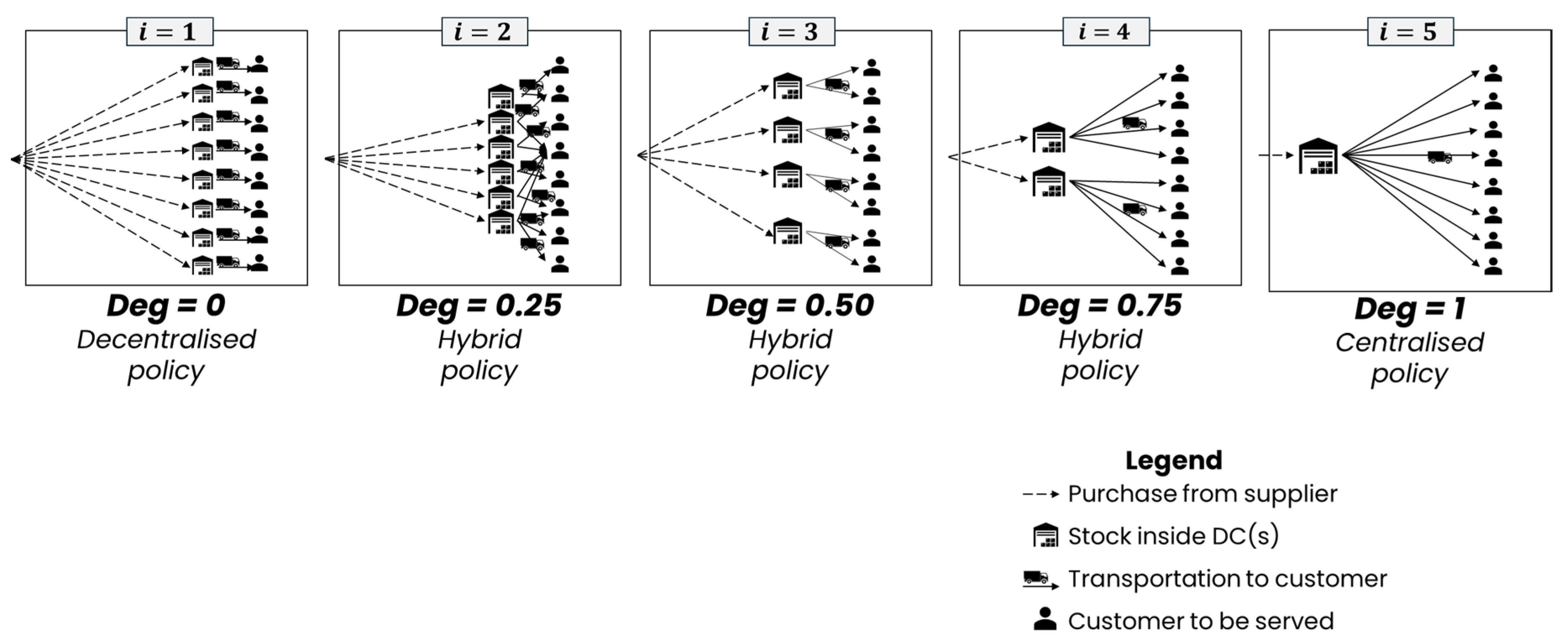
Regarding stock deployment policies ($i$), according to refs. [9,10], they can be distinguished through a parameter called ‘degree of centralisation’ ($De{g}_i$). $De{g}_i$ ranges from 0 to 1, where 0 is decentralisation, 1 is centralisation, and intermediate values represent hybrid stock deployment policies. As expressed in Equation (1), $De{g}_i$ is determined by the ratio between the number of DCs ($D{C}_i$) that can serve customer demand and the total number of customers to be served ($N$). In this work, we focus on comparing five stock deployment policies ($i=1, 2, 3, 4, 5$), including one centralised, one decentralised, and three hybrid options (as schematically illustrated in Figure 1 for an example company with eight customers). This choice is made to enable direct comparison with the only literature study addressing combined stock deployment and manufacturing technology decisions in spare parts DNs [29]. Nevertheless, the present study can be extended to other stock deployment policies since the mathematical equations provided in Section 3.2.1 are general enough to accommodate any value of $De{g}_i$.

$$De{g}_i=\left\{\begin{array}{cc}1,\hfill & if i=5 \left(centralisation\right)\hfill \\ 1-{\displaystyle \frac{D{C}_i}{\mathrm{N}}},\hfill & else\hfill \end{array}\right.$$

(1)

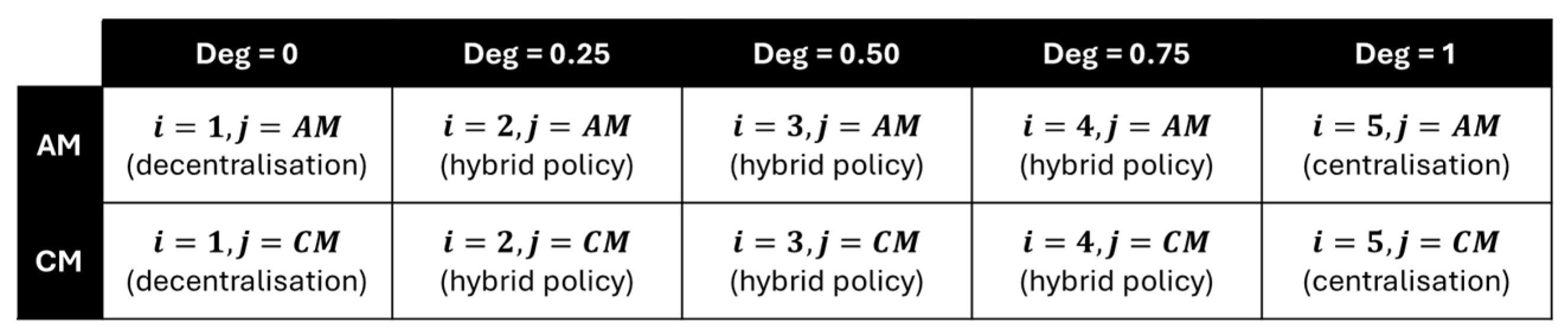
On top of the five stock deployment policies considered, since spare parts can be produced through two manufacturing technologies ($j= AM \mathrm{o}\mathrm{r} CM$), this work aims to support companies in identifying the most cost-effective alternative among the ten listed in Figure 2.

3.2. Three-Step Methodology

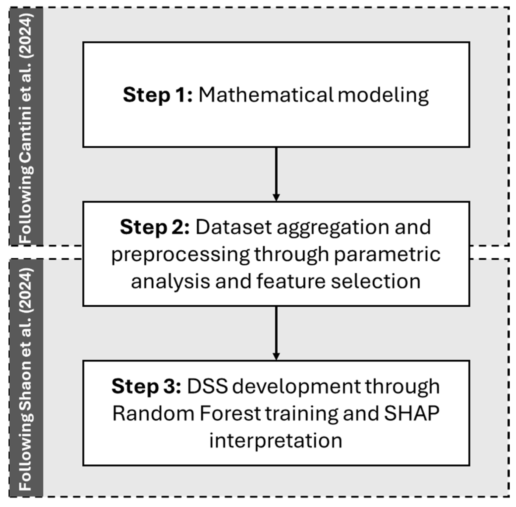
To address the above problem, this work follows the three-step methodology summarised in Figure 3, derived by integrating insights from two seminal studies [29,71].

In Step 1, the mathematical model by [29] served as the foundation for training the DSS. Although this mathematical model associates individual SKUs with the most cost-effective combination of stock deployment and manufacturing technology, it requires solving equations that (as discussed in Section 1) may not be accessible for spare parts retailers lacking advanced mathematical or computational skills. Therefore, while this mathematical model provided the theoretical basis for the DSS, it was not directly considered as the DSS itself.

In Step 2, following ref. [29], a parametric analysis was performed to test the mathematical model on a sample of realistic case studies (i.e., scenarios of spare parts DNs with different demand, costs, service level requirements, etc.). For each scenario, the mathematical model determined the optimal combination of stock deployment policy and manufacturing technology, generating a comprehensive dataset of inputs (i.e., spare parts DN scenarios) and corresponding optimal solutions (i.e., cost-effective combinations of stock deployment policies and manufacturing options). The scenarios for the parametric analysis were intentionally developed following the same procedure as ref. [29] to obtain a similar dataset and be allowed to compare our DSS with the one already existing in the literature (see Section 2). To refine the obtained dataset, following both refs. [29,71], an analysis of variance (ANOVA) was employed to select the variables that significantly influenced the mathematical model outcomes while excluding the negligible ones.

Finally, in Step 3, following ref. [71], the refined dataset was used to feed a Random Forest model aimed at suggesting the optimal combination of stock deployment and manufacturing technology for different spare parts DNs. To ensure a user-friendly and interpretable DSS, SHAP was applied post hoc to explain the logic underlying Random Forest recommendations, thereby ‘opening the black box’.

Below, each step of the proposed methodology is explained in a dedicated sub-section.

3.2.1. Step 1: Mathematical Modelling for Stock Deployment and Manufacturing Technology Decisions

As discussed in Section 2.1, Cantini et al. [29] presented the only prior study addressing joint stock deployment and manufacturing technology decisions in spare parts DNs. Their work introduced a mathematical model to assist retailers in choosing among centralised, decentralised, or hybrid DNs for spare parts produced via AM or CM. This mathematical model is taken as the starting point of this study for two reasons. First, it is well-suited to accomplishing Step 1 of the methodology outlined in Figure 3. Second, using the same model enables a direct comparison between the DSS developed here and the one already available in the literature. Before delving into the model formulation, it is worth noting that the methodology proposed in this work (Figure 3) is not strictly dependent on the mathematical model by Cantini et al. [29]. It can also be applied to other, possibly more advanced formulations (i.e., with fewer simplifying assumptions), should these be developed in the future.

Below, we summarise the formulation of the mathematical model proposed by ref. [29], which relies on the notation reported in

Table 1. List of notations adopted in the mathematical model.

Indexes	Description	Unit Measure
$i$	Considered stock deployment policy. $i$ assumes integer values between 1 and 5 according to Figure 1.	-
$j$	Manufacturing technology of the purchased spare parts. j can be AM or CM.	-
Input Parameters	Description	Unit Measure
$De{g}_i$	Degree of centralisation associated with the stock deployment policy $i$. According to Figure 1, it ranges between 0 and 1.	-
$SL$	Service level pre-established for the specific SKU. It represents the fill rate, calculated as the ratio between the number of demands satisfied on time and the total demands received for that SKU.	-
$\overline{D}$	Average annual demand emitted by one customer for the SKU.	units/time
$N$	Total number of customers served by the DN.	-
$b$	Unitary backorder cost of the considered SKU.	€/backorder
$l_j$	Average procurement lead time needed by the supplier to deliver the j-th SKU to DCs.	time
$c_j$	Unitary cost of purchasing the j-th SKU from the supplier.	€/unit
$o$	Cost of issuing one stock replenishment order.	€/order
$h$	Annual holding cost rate for keeping inventory of the SKU in a DC.	time−1
${et}_{central}$	Unitary transportation cost to deliver the SKU from the central DC to customers. It only refers to the centralised stock deployment policy ($i = 5$).	€/trasportation
Support Variables	Description	Unit Measure
$Q_{i,j}$	Optimal order quantity of the SKU in each DC.	units
${RP}_{i,j}$	Reorder point associated with the SKU in each DC.	units
${SS}_i$	Safety stocks of the SKU in each DC.	units
$D{C}_i$	Total number of DCs in the DN.	-
$D_i$	Total annual demand received by an individual DC for the specific SKU under consideration. It depends on the total number of customers served by the DC.	units/time
${et}_i$	Unitary transportation cost to deliver to SKU from a DC to customers.	€/trasportation
$N_{b_i}$	Average number of annual backorders for the SKU in a DC.	backorders/time
$N_{o_{i,j}}$	Average number of annual orders issued for the SKU in a DC.	orders/time
Decision Variables (Cost Items)	Description	Unit Measure
$C_{{TOT}_{i,j}}$	Total (annual) logistic cost of the DN considering a specific combination of stock deployment policy ($i$) and manufacturing technology ($j$) for the j-th SKU.	€/time
$C_{P_{i,j}}$	Annual purchase cost for the SKU.	€/time
$C_{H_{i,j}}$	Annual holding cost for the SKU.	€/time
$C_{O_{i,j}}$	Annual ordering cost for the SKU.	€/time
$C_{B_{i,j}}$	Annual backorder cost for the SKU.	€/time
$C_{T_{i,j}}$	Annual transportation cost for the SKU.	€/time

. In all equations, the index $i$ denotes the stock deployment policy under consideration (Figure 1), while $j$ is a binary index identifying the manufacturing technology used to produce the SKU, AM or CM. While we provide an overview of this reference model, the reader is referred to ref. [29] for a more detailed description of its equations, as an in-depth analysis lies beyond the scope of this study.

The considered mathematical model supports joint stock deployment and manufacturing technology decisions within a single-period (one-year), single-product setting. In other words, each SKU is analysed individually and assigned to the alternative in Figure 2 that meets predefined service levels while minimising the total (annual) logistic distribution cost ($C_{{TOT}_{i,j}}$). This problem translates into solving the objective function in Equation (2), which aims to identify the minimum $C_{{TOT}_{i,j}}$ among those associated with the ten combinations of stock deployment policies and manufacturing technologies in Figure 2. Once the minimum $C_{{TOT}_{i,j}}$ is determined, the model returns the corresponding values of $i$ and $j$, thereby recommending the most cost-effective solution for the considered SKU. As clarified in Equation (3), $C_{{TOT}_{i,j}}$ is the sum of several cost items, including the cost for purchasing stocks from suppliers (${C_P}_{i,j}$, Equation (4)), the inventory holding cost (${C_H}_{i,j}$, Equation (5)), the ordering cost for replenishing DCs (${C_O}_{i,j}$, Equation (6)), the backorder cost (${C_B}_{i,j}$, Equation (7)), and the transportation cost for delivering products to customers (${C_T}_{i,j}$, Equation (8)).

$$\mathit{min}\left[C_{{TOT}_{i,j}}\right]\hspace{1em}for\hspace{1em}i=\mathrm{1,2},\dots ,5 and j=AM, CM,$$

(2)

$$C_{{TOT}_{i,j}}=C_{P_{i,j}}+C_{H_{i,j}}+C_{O_{i,j}}+C_{B_{i,j}}+C_{T_{i,j}},$$

(3)

where

$$C_{P_{i,j}}=c_j·D_i·D{C}_i,$$

(4)

$$C_{H_{i,j}}=h·c_j·\left({\displaystyle \frac{Q_{i,j}}{2}}+S{S}_{i,j}\right)·D{C}_i,$$

(5)

$$C_{O_i}=o·N_{o_{i,j}}·D{C}_i,$$

(6)

$$C_{B_{i,j}}=b·N_{b_i}·D{C}_i,$$

(7)

$$C_{T_{i,j}}={et}_i·D_i·D{C}_i,$$

(8)

The cost items in Equations (4)–(8) can be derived from Equations (9)–(16), which are valid under the following assumptions (substantiated by scientific literature): (i) Spare parts are purchased from external suppliers (not produced in-house). The purchasing cost of the SKU ($C_{P_{i,j}}$) includes all costs incurred by suppliers, comprising production costs, quality control costs, fixed costs of AM/CM equipment, costs related to the digitalisation of AM items (converting 2D drawings into 3D designs), and the profit margins required by suppliers [72]. (ii) Suppliers’ lead time is deterministic and depends on the SKU, not on the geographical location of DCs [73]. (iii) As already stated at the beginning of this Section, the analysis is conducted over a one-year time horizon and adopts a single-item approach, whereby the most cost-effective stock deployment and manufacturing technology are selected independently for each SKU [3,50]. (iv) No capacity constraints are considered for suppliers’ warehouses or retailers’ DCs [4]. Consequently, each facility can store inventory without space limitations. (v) Customer demand is stochastic and follows a Poisson distribution, which is typical for spare parts [3,74]. (vi) For a given stock deployment policy, the annual demand of all customers is evenly distributed among DCs. (vii) A continuous ($RP,Q$) inventory policy is used to control inventories at DCs [7,75,76], where $RP$ is the reorder point, $Q$ is the optimal order quantity. Moreover, $S{S}_{i,j}$ are the safety stocks corresponding to the smallest value that satisfies Equation (16), thus compensating for demand fluctuations and preventing stock-outs at least to ensure the desired service level. The ($RP,Q$) inventory policy is selected in accordance with [7,76], who recommend its use for managing spare parts with stochastic demand and deterministic lead time. (viii) Lateral transshipments between DCs are not allowed [73,77]. (ix) Reverse logistics (i.e., the repair and reuse of broken spare parts) is not considered, as suggested by [78], because this study does not focus on sustainability issues in DNs, but rather on the selection of cost-effective stock deployment policies and manufacturing technologies for spare parts. (x) The same type of vehicle is used to transport products in all stock deployment policies, with a unit transportation cost assumed to be constant per kilometre [76]. Moreover, transportation costs in decentralised DNs are considered negligible, as each decentralised DC is supposed to be close to the customer it serves. (xi) Only one spare part is shipped per trip. This assumption is reasonable given that spare parts demand follows a Poisson distribution, also known as the law of rare events. (xii) No fixed costs for purchasing or renting DCs are considered, as retailers already own these facilities and the decision problem focuses on determining in which DCs the SKUs should be allocated [79]. (xiii) SKUs are assumed to be producible using both AM and CM in order to enable the comparative analysis presented in this paper. However, if certain parts cannot be produced via AM (as noted in [78]), the considered mathematical model remains applicable by restricting the comparison to the alternatives with $j=CM$ in Figure 2. Methods for identifying spare parts suitable for AM are provided in the literature [80,81].

$$D_i={\displaystyle \frac{\overline{D}·N}{D{C}_i}},$$

(9)

$${DC}_i=\left\{\begin{array}{c}\hfill 1, if i=5\\ \hfill {\left[\left(1-De{g}_i\right)·N\right]}^{+}, else \end{array}\right.,$$

(10)

$$N_{o_{i,j}}={\displaystyle \frac{D_i}{Q_{i,j}}},$$

(11)

$$N_{b_i}={\left[\left(1-SL\right)·D_i\right]}^{+},$$

(12)

$${et}_i=\left\{\begin{array}{c}\hfill {et}_{central}, if i=5\\ \hfill (0.7644\ast {Deg}_i^2+0.2009\ast De{g}_i+0.0161)·{et}_{central}, else \end{array}\right.,$$

(13)

$$Q_{i,j}=\sqrt{{\displaystyle \frac{2·D_i·o}{h·c_j}}},$$

(14)

$$R{P}_{i,j}=D_i·l_j+{SS}_{i,j},$$

(15)

$$1-{\sum }_{n=0}^{S{S}_{i,j}-1}\left[{\displaystyle \frac{{\left(D_i·l_j\right)}^n}{n!}}·e^{-\left(D_i·l_j\right)}\right]\ge (1-SL),$$

(16)

3.2.2. Step 2: Dataset Aggregation and Preprocessing Through Parametric Analysis and Feature Selection

In Step 2 of the methodology (Figure 3), a parametric analysis was conducted to test the mathematical model across realistic case studies (i.e., DN scenarios varying in spare parts demand, costs, service levels, etc.). The scenarios for the parametric analysis were generated following the same procedure as in ref. [29], namely by assigning Sobol quasi-random values to the independent input parameters of the mathematical model (see Table 1). The only exceptions were $De{g}_i$, which already had predefined values (see Figure 1), and $o$ and $h$, which were fixed at 5 €/order and 25% of the SKU purchase cost ($c_j$), respectively. According to Equation (17), the Sobol quasi-random low-discrepancy sequence was used to vary input parameters ($par$) and assign them uniformly distributed values within the ranges specified in Table 2. As reported by refs. [82,83], in Equation (17),$K$ denotes the total number of values assigned to each input parameter, and $k$ represents a specific generated value. $P$ indicates the total number of input parameters in the mathematical model, while $p$ refers to the specific input parameter to which a Sobol value ($pa{r}_{pk}$) is assigned. $S_{pk}$ is the Sobol sequence, and $l{l}_p$ and $u{l}_p$ denote the lower and upper bounds defining the admissible range of the input parameter (Table 2).

The parameter ranges (i.e., $l{l}_p$ and $u{l}_p$ in Table 2) were selected to balance two objectives: ensuring a realistic representation of spare parts DN scenarios and enabling comprehensive exploration of the decision space. Each range is grounded in prior empirical research, as documented in the last column of Table 2. Moreover, adopting identical ranges, Cantini et al. [29] enabled direct comparison with existing literature, ensuring that any performance differences between our DSS and the existing decision tree-based DSS reflect algorithmic improvements rather than artefacts of different training data.

The Sobol quasi-random low-discrepancy sequence was chosen to generate DN scenarios because, as highlighted by [84], when dealing with problems involving numerous input parameters, it offers a sampling strategy that explores the design space (i.e., the space of admissible input parameter combinations) more uniformly than other sequences (e.g., discrete sampling, Latin Hypercube, or Monte Carlo). Nevertheless, the validity of the proposed methodology remains preserved if alternative sampling strategies are employed.

$$pa{r}_{pk}=l{l}_p+S_{pk}·\left({ul}_p-l{l}_p\right)\hspace{1em}\hspace{1em}\hspace{1em}with p=1,\dots ,P and k=1,\dots ,K,$$

(17)

For each generated scenario, the mathematical model was applied to determine the optimal combination of stock deployment policy ($i=1-5$ in Figure 1) and manufacturing technology (j = AM or CM), out of the ten combinations of Figure 2. This resulted in the generation of a dataset of 2000 realistic case studies described by inputs (i.e., spare parts DN scenarios) and the corresponding optimal solutions (i.e., cost-effective combinations of stock deployment policies and manufacturing options).

Table 2. Ranges of Sobol values allowed for each input parameter.

Input Parameters	Range of Admissible Values	Unit Measure	Literature References
$N$	integers between 5 and 100	-	[4,20,29]
$SL$	floats between 0.85 and 0.99	-	[3,4,29]
$\overline{D}$	integers between 1 and 7	units/year	[29,85]
$b$	floats between 1000 and 100,000	€/backorder	[29,86]
$l_{AM}$	integers between 1 and 4	weeks	[24,29,85]
$l_{CM}$	integers between 4 and 26	weeks	[24,29,85]
$c_{AM}$	floats between 100 and 2500	€/unit	[29,85]
$c_{CM}$	floats between 10 and 2500	€/unit	[29,85]
${et}_{central}$	floats between 100 and 2000	€/transportation	[25,29]

Table 2. Ranges of Sobol values allowed for each input parameter.

Input Parameters	Range of Admissible Values	Unit Measure	Literature References
$N$	integers between 5 and 100	-	[4,20,29]
$SL$	floats between 0.85 and 0.99	-	[3,4,29]
$\overline{D}$	integers between 1 and 7	units/year	[29,85]
$b$	floats between 1000 and 100,000	€/backorder	[29,86]
$l_{AM}$	integers between 1 and 4	weeks	[24,29,85]
$l_{CM}$	integers between 4 and 26	weeks	[24,29,85]
$c_{AM}$	floats between 100 and 2500	€/unit	[29,85]
$c_{CM}$	floats between 10 and 2500	€/unit	[29,85]
${et}_{central}$	floats between 100 and 2000	€/transportation	[25,29]

As suggested by refs. [29,71], an ANOVA was performed to refine the dataset by identifying which input parameters significantly influence the optimal stock deployment and manufacturing technology decisions. The objective was to determine whether all input parameters of the mathematical model (Table 1) had a significant impact on the model output (i.e., suggestion of the optimal combination of stock deployment and manufacturing technology) or whether some parameters exhibited negligible effects. Accordingly, the ANOVA supported both model parsimony (by eliminating non-influential variables) and practical guidance for retailers by distinguishing critical operational variables from those that can be approximated without loss of decision quality.

The ANOVA was conducted following the same procedure established in ref. [29]. The input parameters listed in the first column of Table 2 were treated as independent input factors, while the optimal combinations of stock deployment and manufacturing option generated by the mathematical model for the different DN scenarios were used as categorical responses. Consistent with the findings in ref. [29], six parameters were found to have a statistically significant influence on the decision outcomes ($N$, $\overline{D}$, $b$, $c_{AM}$, $c_{CM}$, and ${et}_{central}$), whereas three parameters ($SL$, $l_{AM}$, and $l_{CM}$) showed negligible effects. Since our results confirmed pre-existing literature, to avoid redundancy, readers are referred to ref. [29] for a more detailed discussion of the ANOVA outcomes. Here, we only summarise the main results relevant to this study.

Among the influential parameters, the unit transportation cost under centralised DNs (${et}_{central}$) emerged as a strong influential factor, driving the trade-off between inventory aggregation (i.e., centralisation) and customer proximity (i.e., decentralisation). Also, the unit costs of AM and CM parts ($c_{AM}$ and $c_{CM}$) emerged as highly influential, and this reflects that AM and CM cost competitiveness directly affects both the technology selection and the feasibility of degrees of centralisation. Similarly, the backorder cost ($b$) showed statistically significant effects on the decision-making problem, revealing the service-responsiveness trade-off in DNs. Finally, demand-related parameters ($N$ and $\overline{D}$) exhibited non-negligible effects, indicating that market and demand size shape both stock deployment and manufacturing choices, as they determine whether sufficient volume exists to justify investments in distributed capacity.

Conversely, $SL$, $l_{AM}$, and $l_{CM}$ showed negligible impacts on the outcomes of the mathematical model within the tested ranges (Table 2). In fact, service level requirements ($SL$) are already captured through economically weighted backorder penalties ($b$), making the $SL$ parameter redundant. Similarly, AM’s lead time advantage over CM is already embedded in the technology choice variable ($j$), making $l_{AM}$, and $l_{CM}$ redundant without adding explanatory power. Based on these ANOVA results, the variables with a negligible effect were excluded from the dataset. Conversely, the remaining input parameters (with a significant influence) were retained. The refined dataset (available in the Supplementary Materials) served as the input for training the DSS, as described below.

3.2.3. Step 3: DSS Development Through Random Forest Training and SHAP Interpretation

In Step 3 of the methodology (Figure 3), the DSS was developed through two sequential subtasks. First, a Random Forest model was trained using the dataset obtained from Step 2. Then, the Random Forest recommendations on stock deployment and manufacturing technology were explained post hoc to enhance their user-friendliness and interpretability.

As anticipated, the Random Forest was selected as the ML model because, as reported by refs. [87,88], it employs an ensemble of decision trees to suggest the class to which an instance belongs (in this case, the optimal combination of stock deployment policy and manufacturing technology among the ten alternatives in Figure 2) based on a set of features (namely, the input parameters characterising each DN scenario and showing a non-negligible impact on the mathematical model). Owing to its ensemble nature, Random Forest is well-suited to capturing complex interactions among variables and typically outperforms single decision trees by reducing overfitting and improving generalisation through the random selection of both data samples and features during tree construction [60]. Following refs. [24,89], Random Forest was employed as a classification model and trained on the full dataset generated in Step 2 to capture the effects of input features on stock deployment and manufacturing technology decisions across different DN scenarios.

The Random Forest was trained using hyperparameters determined through a synthesis of preliminary empirical testing and established best practices for classification [90]. Specifically, we employed the Gini impurity as the criterion for node splitting. The forest was composed of 100 estimators to ensure a trade-off between classification performance and computational overhead. No explicit constraint was placed on the maximum tree depth, as the dataset size (2000 observations) was not excessively large to incur overfitting risks. Moreover, deeper trees capture high-order interactions among DN parameters. Furthermore, the minimum samples per split were maintained at the default value of two, enabling the detection of fine-grained patterns in the data while preventing excessive leaf fragmentation.

The Random Forest performance was evaluated in terms of accuracy, computed (according to Equation (18)) as the ratio between the number of correct recommendations consistent with the mathematical model results ($Nc{r}_{RF}$) and the total number of recommendations corresponding to the initial dataset size ($Nt{r}_{RF}$). In addition, a confusion matrix was generated to break down the true and false positive classifications.

Table 3. Confusion matrix associated with the trained Random Forest.

		Recommended Label Out of the Ten Combinations (i,j) in Figure 2
		1	2	3	4	5	6	7	8	9	10
True Label Out of the Ten Combinations (i,j) in Figure 2	1	213	0	0	16	0	3	0	1	0	0
	2	0	10	0	0	0	0	2	0	0	0
	3	0	0	120	0	17	0	7	0	0	0
	4	18	0	0	757	0	13	0	2	0	0
	5	0	2	14	0	617	0	5	0	1	0
	6	0	0	0	7	0	76	0	3	0	0
	7	0	3	2	0	8	0	40	0	1	0
	8	0	0	0	3	0	1	0	27	0	0
	9	0	1	0	0	1	0	1	0	7	0
	10	0	0	0	1	0	0	0	0	0	0

reports the results of the training process, highlighting correctly classified DN scenarios along the bold diagonal of the matrix. According to Table 3, 1867 DN scenarios were correctly classified by the Random Forest, with only 133 misclassifications. This resulted in an accuracy of 93.4%, confirming improved performance compared to the 77.0% accuracy of the decision tree-based DSS proposed by ref. [29].

$$A_{RF}={\displaystyle \frac{Nc{r}_{RF}}{{Ntr}_{RF}}}$$

(18)

Unlike decision trees, the Random Forest functions as a black box, producing accurate recommendations on stock deployment and manufacturing technology without explicitly revealing the reasoning behind them. To make the DSS more user-friendly and interpretable, SHAP was employed to provide post hoc explanations of Random Forest recommendations. SHAP was selected as the XAI model because it enhances both global and local interpretability through ‘SHAP values’, which quantify the contribution of each feature (i.e., input parameter) to the Random Forest recommendations [91,92]. Specifically, ‘SHAP summary plots’ visualise the average impact of each feature across all observations (i.e., DN scenarios), while ‘SHAP waterfall plots’ enable a local analysis by highlighting the specific contribution of individual features to the recommendation for a single observation [68]. This combination of global and local perspectives allows spare parts retailers to interpret the DSS recommendations at both macro and micro levels, improving transparency of stock deployment and manufacturing technology decisions generated by the Random Forest. Overall, the joint use of the Random Forest (to recommend the optimal alternative among the ten in Figure 2) and SHAP plots (to interpret the underlying rationale) results in an accurate and interpretable DSS.

4. Results

This section presents the DSS, which integrates Random Forest recommendations with SHAP-based visual interpretations.

Concerning Random Forest, it has already been described in Section 3.2.3, detailing its inputs, outputs, and performance metrics. In practice, retailers can consult the Random Forest by providing it with the input parameters listed in Table 1 (each filled with values representing the specific characteristics of their DN). Based on these inputs, Random Forest recommends the most cost-effective combination of stock deployment policies and manufacturing options (among the ten alternatives in Figure 2), ensuring a prediction accuracy of 93.4% (a + 16.4% improvement over the decision-tree-based DSS of [29]). While this performance improvement may appear as a technical metric, its managerial implications are substantial. When the DSS incorrectly recommends a suboptimal combination of stock deployment policy and manufacturing technology, retailers incur unnecessary logistics costs relative to the truly optimal solution. Our Random Forest-based DSS generates 133 misclassifications (6.6% error rate), compared to 460 misclassifications (23.0% error rate) produced by the literature DSS [29], resulting in 327 fewer erroneous recommendations across the 2000-scenario dataset. To quantify the economic impact, we examined the cost differentials between recommended and optimal solutions for misclassified cases, finding that our DSS produces an average cost penalty of €3008 per misclassification (with a standard deviation of ±€229). For the sake of comparability, this same average penalty was assumed for the decision-tree-based DSS [29], in order to isolate the economic effect of different classification accuracies. Considering, as an example, a medium-sized retailer managing 1000 SKUs, the decision-tree-based DSS (with 77.0% accuracy, namely ~230 misclassifications over 1000 predictions), would generate annual excess costs of about €692,000 (230 × €3008). In contrast, our Random Forest-based DSS (with 93.4% accuracy, namely ~66 misclassifications over 1000 predictions) would generate annual excess costs of around €199,000 (66 × €3008), yielding a net annual saving of €493,000.

Beyond direct cost savings, the accuracy improvement fundamentally changes how managers interact with and trust the DSS. As reported by refs. [32,66], a low accuracy fosters managerial scepticism and limits ML adoption to selective, expert-supervised uses. The high error rate necessitates constant oversight, restricting scalability and preventing systematic deployment across organisational units. Conversely, a high accuracy (93.4%) encourages retailers to confidently implement the DSS recommendations, standardising decision-making across multiple DCs, training junior staff by using DSS recommendations as learning tools, and reducing dependence on individual expert judgement. The combination of cost savings and organisational confidence makes the accuracy improvement strategically significant rather than merely technically noteworthy.

After training the (black box) Random Forest, SHAP-based interpretations of the ML recommendations are provided through two types of plots: (i) ‘SHAP waterfall plots’ for local-level interpretations, which visually illustrate the reasoning behind the Random Forest suggestions for a specific DN under analysis; and (ii) ‘SHAP summary plots’ for global-level interpretations, which show the average importance of each input parameter (feature) across the entire dataset, thereby providing insights applicable to generic DNs. Each visualisation type is described below, along with guidance on interpretation, to ensure that the DSS remains both accessible and actionable for spare parts retailers.

4.1. Waterfall Plots: Local-Level Interpretations

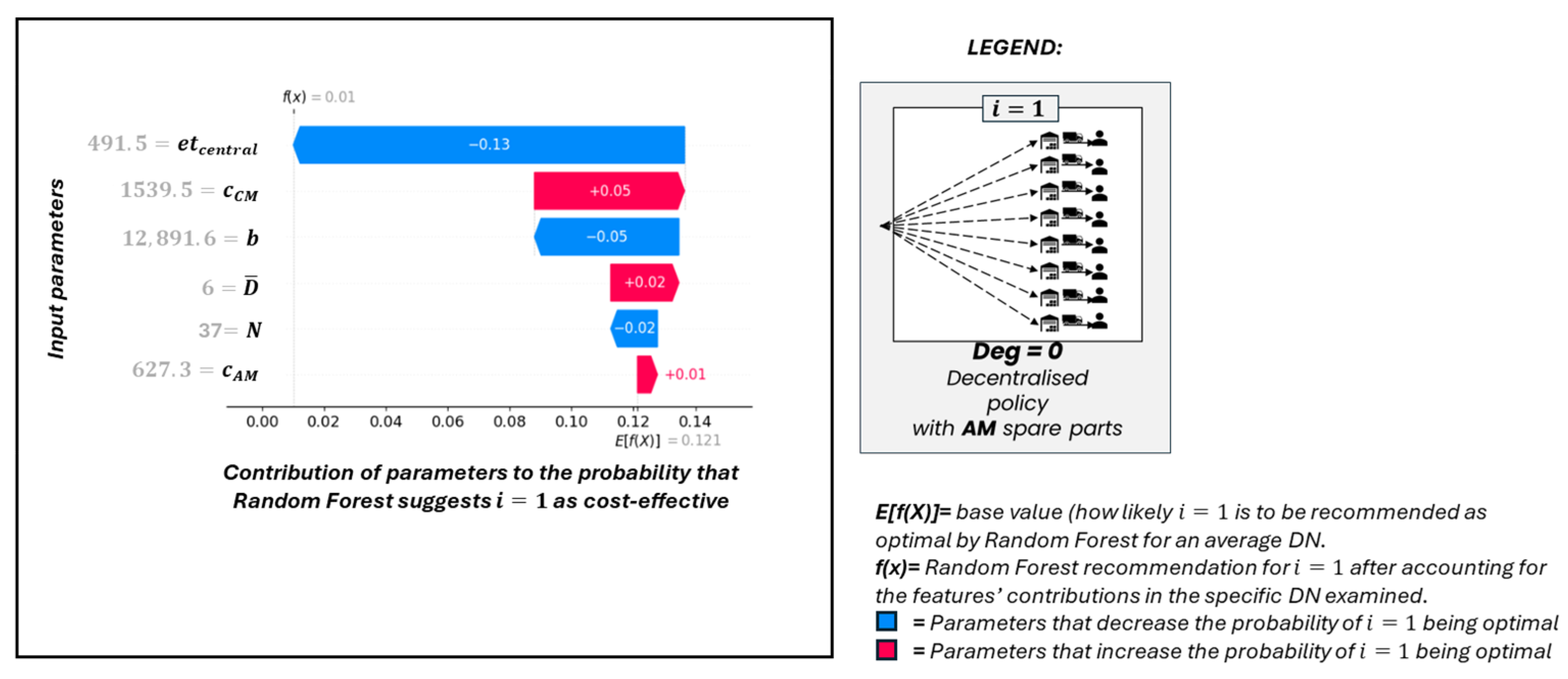
SHAP waterfall plots provide local explanations by showing how individual input parameters contribute to the Random Forest recommendations for a specific DN scenario. Figure 4 illustrates an example waterfall plot for the first DN scenario in the training dataset, focusing on interpreting the Random Forest recommendations regarding the first configuration in Figure 2 (i.e., decentralised stock deployment policy with AM spare parts, schematically depicted on the right of Figure 4).

The plot visualises the Random Forest recommendation process as follows. The y-axis displays the actual values of each input parameter (a.k.a. feature) for the specific DN scenario under analysis. For instance, Figure 4 refers to a DN with 37 customers, each having an average demand of 6 product units/year, and so on.

$E\left[f\right(X\left)\right]$ (bottom right in Figure 4, equal to 0.121) represents the base value (baseline), given by the average SHAP model output for the first configuration of Figure 2 to be selected as optimal across all observations in the training dataset (DN scenarios). This baseline serves as the starting point for understanding how likely the first configuration of Figure 2 is to be recommended as optimal by the Random Forest in the absence of specific feature information for the analysed DN scenario.

Next, $f\left(X\right)$ (top left in Figure 4, equal to 0.01) represents the final Random Forest recommendation for the first configuration of Figure 2 after accounting for all feature contributions from the specific DN scenario being examined. A higher $f\left(X\right)$ value indicates a greater likelihood that the Random Forest recommends decentralisation of AM spare parts for this DN scenario, and vice versa. The low value of $f\left(X\right)=0.01$ (compared to the baseline of $E\left[f\left(X\right)\right]=0.121$) clearly indicates that the first configuration of Figure 2 is highly unlikely to be cost-effective for the first DN scenario in the dataset.

Each coloured bar in Figure 4 corresponds to one feature (input parameter), with its length and colour indicating the magnitude and direction of its contribution to the Random Forest recommendation. Blue bars with negative values decrease the likelihood of the first configuration of Figure 2 being optimal (pushing the recommendation away from decentralised AM toward other configurations of Figure 2), while red bars with positive values increase this likelihood (pushing toward decentralisation of AM spare parts). The longer the bar, the greater the impact of that input parameter on the final Random Forest recommendation.

Notably, $f\left(X\right)$ is always equal to $E\left[f\right(X\left)\right]$ plus the sum of all feature contributions. For example, if the second bar corresponds to +0.02, this means that the average customer demand of 6 units/year increased the decentralisation recommendation ($f\left(X\right)$) by 0.02 compared to the average baseline $E\left[f\right(X\left)\right]$.

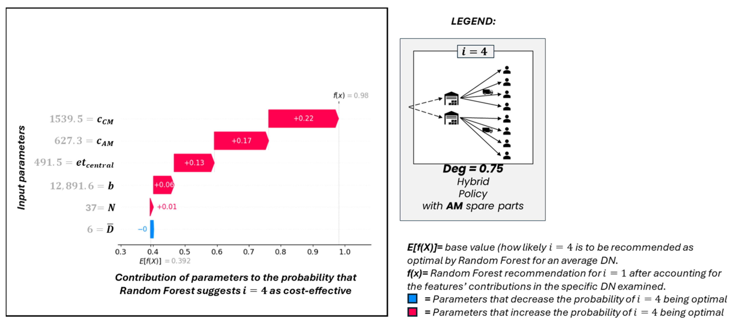
As another example, Figure 5 shows the waterfall plot for the same DN scenario (first row of the dataset), considering the Random Forest recommendation for the fourth configuration in Figure 2 (i.e., hybrid stock deployment policy with $De{g}_i=0.75$ and spare parts produced via AM, schematically depicted on the right of Figure 5). In Figure 5, the high value of $f\left(X\right) = 0.98$ (compared to the baseline $E\left[f\right(X\left)\right] = 0.392$) confirms that the fourth configuration of Figure 2 is likely to be the most cost-effective for the considered DN scenario. The waterfall plot reveals the reasoning behind this Random Forest recommendation. As shown in Figure 5, the relatively low transportation cost ($e{t}_{central}$ = 491.5 €) provides a strong positive contribution (+0.13, red bar) toward the fourth configuration of Figure 2. This aligns with established literature [10,13], which reports that lower transportation costs favour centralisation as they enable retailers to exploit risk-pooling benefits without excessive delivery expenses. In fact, when transportation is inexpensive, configurations with higher degrees of centralisation (e.g., $De{g}_i=0.75$) become more cost-effective, as there is minimal transportation cost penalty associated with consolidating inventory in fewer DCs serving customers from more distant locations.

In addition, the high CM unit cost ($c_{CM} = 1539.5 €$) provides the strongest positive contribution (+0.22, red bar) to choose the fourth configuration of Figure 2. This finding is consistent with prior research on manufacturing technology selection [23,24], which shows that AM becomes cost-competitive when CM costs are elevated. Indeed, AM spare parts are preferred over CM because they are cheaper, and expensive stocks benefit from risk-pooling effects achieved through higher degrees of centralisation. Since similar considerations can be made for all the other input parameters, the final waterfall plot in Figure 5 demonstrates that the fourth configuration of Figure 2 (hybrid stock deployment policy with $De{g}_i=0.75$ and AM spare parts) is optimal for this DN scenario.

Overall, waterfall plots enable spare parts retailers to understand why a specific combination of stock deployment policy and manufacturing technology was recommended by Random Forest for their DN and for each SKU, thereby strengthening trust in the DSS recommendations. Specifically, managers can follow this step-by-step protocol. First, they input the DN and SKU’s features (e.g., number of customers served, demand per customer, etc.) into the DSS. The Random Forest recommends the optimal stock deployment and manufacturing technology (e.g., hybrid policy with 75% degree of centralisation and AM production). Subsequently, retailers analyse the SHAP waterfall plot (e.g., Figure 5) to understand why this recommendation is generated, identifying both the strongest positive contributors pushing toward the selected solution (e.g., high CM unit costs and low transportation costs) and the negative contributors pushing against it (i.e., no particular ones in the case of Figure 5). The magnitude of the final prediction $f\left(X\right)$ relative to the baseline $E\left[f\right(X\left)\right]$ enables an assessment of decision confidence: a large gap between these two values indicates a robust recommendation. Conversely, $f\left(X\right)$ values close to the baseline $E\left[f\right(X\left)\right]$ highlight ambiguous cases requiring sensitivity analysis or managerial judgement. Finally, based on the outcomes of Random Forest and SHAP, retailers can use the DSS recommendations to make appropriate stock deployment and manufacturing choices. For example, in the case of Figure 5, they can procure AM spare parts from suppliers and stock them in selected regional DCs to balance cost-efficiency and service responsiveness.

4.2. Summary Plots: Global-Level Interpretations

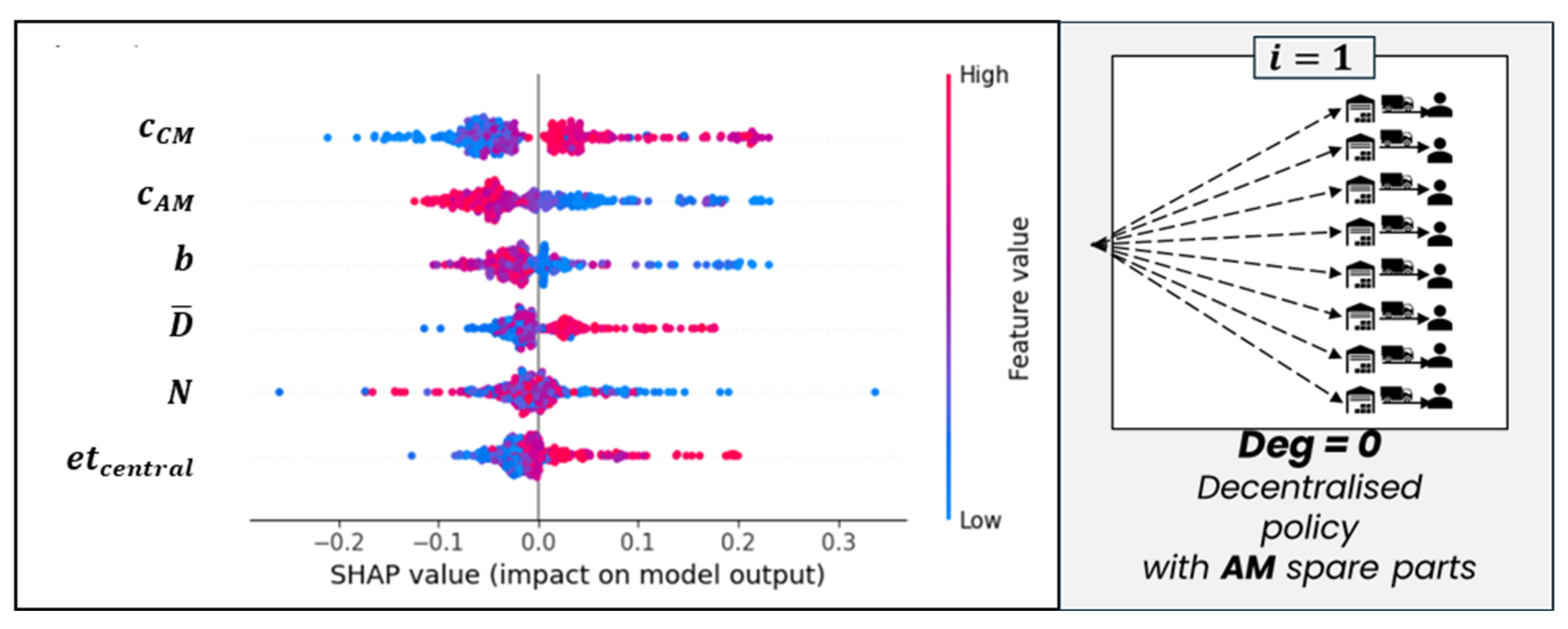
While waterfall plots provide local-level interpretations, summary plots aggregate SHAP values across all DN scenarios in the training dataset to reveal global patterns of feature importance (applicable to any generic DN). Figure 6 presents the SHAP summary plot obtained for the first configuration of Figure 2 (decentralisation of AM spare parts, here schematically represented on the right side of Figure 6).

The structure of Figure 6 is as follows. The vertical axis lists input parameters ranked by their average impact on Random Forest recommendations for the first configuration of Figure 2, with the most influential features positioned at the top. This ranking provides immediate insight into which input parameters most strongly drive the Random Forest recommendation of decentralisation of AM spare parts.

The horizontal axis displays SHAP values, which indicate both the magnitude and direction of each feature’s contribution to the Random Forest recommendation across different DN scenarios (dots). SHAP values to the right of zero (positive values) increase the likelihood that the first configuration of Figure 2 is recommended as optimal, while values to the left of zero (negative values) decrease this likelihood. The distance from zero represents the strength of the contribution.

For each feature on the y-axis, Figure 6 depicts 2000 dots, where each dot represents an individual DN scenario from the dataset. The dot’s position along the x-axis indicates how strongly that feature (y-axis) pushed the recommendation toward or away from the first configuration in Figure 2 for that specific (local) DN scenario. The colour of each dot indicates the feature value for that DN scenario: red represents high feature values, while blue represents low values. This colour-coding enables visual identification of the relationship between feature magnitude and recommendation impact. For instance, a red dot for $c_{AM}$ positioned far left (negative SHAP value) represents a scenario where high AM unit costs strongly discouraged the decentralisation of AM spare parts in favour of alternative configurations of Figure 2. Conversely, a blue dot for $c_{AM}$ positioned far right (positive SHAP value) indicates that low AM costs strongly favoured the decentralisation of AM spare parts for the considered DN scenario.

The distribution pattern of dots reveals critical insights about how feature values relate to recommendation outcomes. If most dots cluster on the positive side of the x-axis (to the right of zero), that feature generally exerts a positive impact on recommending the first configuration of Figure 2. Conversely, if dots concentrate on the negative side (to the left of zero), the feature tends to steer recommendations away from decentralised AM configurations toward other alternatives of Figure 2. For example, in Figure 6, the feature $c_{CM}$ displays red dots predominantly on the positive side and blue dots on the negative side, indicating that higher CM costs favour the decentralisation of AM spare parts, whereas lower CM costs discourage it. In other words, the spread of dots along the x-axis for a given feature reflects how consistently that feature influences Random Forest recommendations across different DN scenarios. A wide horizontal dispersion (as observed for $N$) suggests that the feature’s impact is highly context-dependent and varies significantly based on interactions with other parameters, whereas a narrower distribution (as observed for $\overline{D}$) indicates a more consistent behaviour.

By combining positional information (x-axis) with colour-coding, the summary plot reveals whether high or low values of each feature drive specific recommendation outcomes. For example, if a feature displays predominantly red dots on the positive side of the x-axis, this indicates that high values of the feature consistently increase the probability of recommending the first configuration of Figure 2 for a generic DN. Conversely, if a feature shows red dots clustered on the negative side, this means that high values of this feature push recommendations away from the first configuration of Figure 2 toward more centralised or CM-based configurations. Likewise, if blue dots (low feature values) appear predominantly on the positive side of the x-axis, low values of that feature favour decentralised AM scenarios and vice versa.

According to these interpretation rules, Figure 6 (namely, the SHAP summary plot for the decentralised AM configuration with $i= 1$ and $j=AM$) reveals several insights that both confirm and extend prior findings in the spare parts management literature. First, the unit cost of CM parts ($c_{CM}$) emerges as the most influential feature: lower $c_{CM}$ values (blue dots) reduce the likelihood of recommending decentralised AM (negative SHAP values), whereas higher $c_{CM}$ values (red dots) increase it (positive SHAP values). This confirms Cantini et al.’s [29] earlier observation that relative (AM vs. CM) manufacturing costs dominate stock deployment decisions when AM is considered. However, our SHAP analysis reveals additional nuance: the wide horizontal dispersion of the dots in Figure 6 indicates that when CM is expensive, AM becomes comparatively more attractive, although the impact of this effect varies across DN scenarios, being context-dependent. This finding aligns with ref. [11], which posits that AM adoption in spare parts DNs depends critically on cost competitiveness relative to CM, but our results demonstrate that this relationship is non-linear and influenced by DN-specific characteristics.

The second most influential feature is the unit cost of AM parts ($c_{AM}$), which clearly exhibits a pattern opposite to $c_{CM}$: low AM costs (blue dots) strongly support decentralised AM spare parts and vice versa. Moreover, in agreement with ref. [23], it confirms that decentralised AM is viable only when the manufacturing technology is economically accessible, especially if AM inventories must be kept across multiple DCs (decentralisation).

Analysing the unit backorder cost ($b$), red dots in Figure 6 concentrate on the negative side of the x-axis, meaning that high $b$ values discourage decentralised AM recommendations in favour of more centralised or CM-based DNs. This suggests that when service criticality is high, alternative combinations of stock deployment and manufacturing strategies may outperform decentralisation. This finding may appear counterintuitive as some authors [12,14] suggest that high service requirements favour decentralisation for responsiveness. However, our results show a more sophisticated dynamic: when backorder costs are extreme, centralised DNs for AM spare parts may provide superior service by benefiting from risk-pooling (compensating demand fluctuations and, thus, limiting backorders) while still offering shorter lead times than CM and without requiring the inventory replication costs of decentralisation. This explanation is consistent with supply chain theory [11,22] and reconciles the apparent contradiction with prior literature.

The average annual demand per customer ($\overline{D}$) is associated mainly with red dots on the positive x-axis, indicating that high $\overline{D}$ values consistently increase the likelihood of recommending the first configuration in Figure 2. This suggests that sufficient local demand volume is required to justify distributed investment management.

Unexpectedly, the number of customers ($N$) has a relatively modest impact on Random Forest recommendations. This implies that demand density, backorder costs, and purchasing costs weigh more heavily than the sheer number of customers, a distinction not explicitly made in prior qualitative works [23]. In fact, red and blue dots are scattered along the x-axis of Figure 6, indicating that, although geographically dispersed customers may favour decentralised stock deployment policies, the influence of $N$ is dependent on its interaction with other features and varies across DN scenarios.

Finally, the unit transportation cost under centralisation (${et}_{central}$) shows an intuitive pattern: high transportation costs favour decentralised AM (positive SHAP values), though, again, the magnitude of this effect depends on interactions with other features. This confirms classical location theory [4,18], expanding it by showing (through the horizontal dispersion of dots in Figure 6) that transportation costs alone do not determine optimal stock deployment and manufacturing technology decisions. Rather, their influence depends heavily on interactions with manufacturing costs, demand patterns, etc.

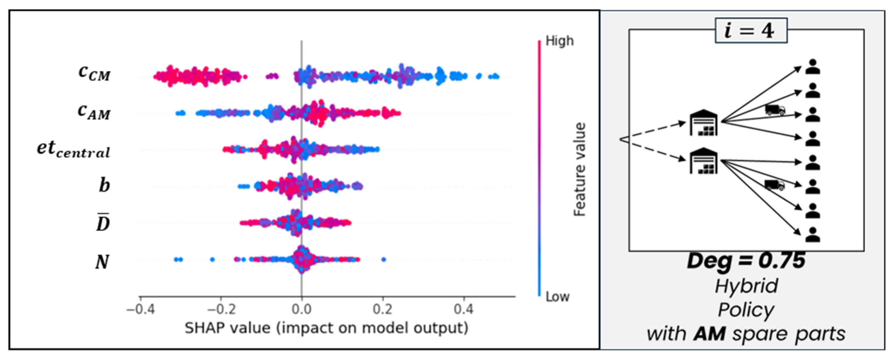
Similar considerations arise from Figure 7, which—consistent with Figure 5—provides another SHAP summary plot explaining the recommendations for the fourth configuration in Figure 2 (i.e., hybrid stock deployment policy with $De{g}_i=0.75$ and AM-produced spare parts, here schematically depicted on the right side of Figure 7). In this case, the patterns associated with $c_{CM},$ $c_{AM}$ and $\overline{D}$ are reversed relative to Figure 6, because the plot illustrates the tendency to recommend a stock deployment policy with a high degree of centralisation ($De{g}_i=0.75$), rather than the previously analysed decentralisation. A similar inversion is observed for ${et}_{central}$, whose increased relevance compared to Figure 6 suggests that this feature plays a major role in distinguishing among hybrid stock deployment policies (with different degrees of centralisation, $De{g}_i$). By contrast, $b$ and $N$ show red and blue dots interspersed and mostly concentrated around SHAP values close to zero. This pattern suggests that, for recommendations involving hybrid stock deployment policies, the influence of $b$ and $N$ emerges primarily through interactions with other features, making their impact case-specific and dependent on the specific DN under analysis.

While the waterfall plots in Section 4.1 explain individual Random Forest recommendations for specific DN scenarios, the SHAP summary plots offer a global view of feature importance by revealing aggregate patterns of feature influence across the entire dataset (all DN scenarios). These plots enable retailers to derive general guidelines on which DN characteristics favour particular combinations of stock deployment policies and manufacturing technologies for a given SKU. For example, companies facing increasing customer demand (higher $\overline{D}$) or rising fuel expenses for petrol vehicles (higher ${et}_{central}$), combined with rising CM supplier costs (higher $c_{CM}$), should anticipate potential advantages from shifting toward more decentralised stock deployment policies of AM spare parts.

Adopting this global perspective, SHAP summary plots allow managers to extract generalisable decision rules for groups of SKUs rather than analysing each SKU individually. By examining the ranking and colour of features, retailers can identify the dominant decision drivers (e.g., CM unit cost, AM unit cost, backorder cost, etc.) and derive actionable rules such as: (i) when CM costs are high, shift toward AM-based configurations; (ii) when AM costs are low and local demand is high, decentralised AM becomes viable; (iii) when backorder costs are high, centralised AM is preferable to exploit risk-pooling; and (iv) when transportation costs increase, favour decentralisation. These insights enable retailers to monitor triggering conditions that signal the need to reassess stock deployment and manufacturing technology decisions. Accordingly, retailers managing thousands of SKUs can periodically screen the portfolio to identify spare parts affected by changes in features (such as increases in CM prices, reductions in AM costs, or rising demand volumes) and then apply DSS-guided rules to determine whether current stock deployment policies and manufacturing technologies remain appropriate or should be adjusted.

5. Discussion and Conclusions

This study developed a DSS that integrates Random Forest prediction with SHAP-based interpretations to address the RQ: How can ML and post hoc XAI support joint decisions on stock deployment and manufacturing technology in spare parts DNs? The DSS identifies the most cost-effective option among ten alternatives, combining five stock deployment policies (one centralised, one decentralised, and three hybrid) with two manufacturing technologies (AM or CM). While Random Forest ensures prediction accuracy, SHAP provides both local (DN-specific) and global (dataset-wide) visual explanations that clarify the rationale behind recommendations. Together, these elements enable a data-driven, transparent, and actionable DSS that supports alignment between stock deployment and spare parts manufacturing strategies with market needs, and promotes a more informed adoption of AM as a potential substitute for CM.

The DSS builds on prior contributions in the literature ([29,71]) by coupling a cost-based mathematical model with parametric analysis, ML-based classification (Random Forest), and XAI (SHAP). Compared with the only similar DSS in the literature [29], the proposed DSS improves performance, achieving 93.4% accuracy versus 77.0% while relying on the same dataset and underlying mathematical model. This improvement derives from the ensemble nature of Random Forest, which captures complex, non-linear interactions among decision variables that single decision trees cannot represent effectively. Besides predictive performance, the integration of SHAP yields insights that extend beyond those offered by decision-tree-based DSSs. While decision trees explain decisions through a single reasoning path (due to their branching structure, which may oversimplify complex trade-offs), SHAP quantifies the marginal contribution of each input feature across all DN scenarios. In doing so, SHAP reveals interaction effects and differences between local (instance-level) and global (dataset-level) explanations through complementary visualisations (waterfall and summary plots). This is reflected in the changing relative importance of features (i.e., the order on the y-axis) across local and global analyses (Figure 4 vs. Figure 6), as well as across recommendations for different combinations of stock deployment and manufacturing options (Figure 4 vs. Figure 5). Overall, SHAP enables retailers to understand not only ‘what’ combination of stock deployment and manufacturing technology is recommended by the DSS, but also ‘why’, indicating which DN features (customer numbers, costs, demand sizes, etc.) drive each recommendation and how strongly they influence it.

Consistent with prior evidence [29], the DSS results confirm that the unit costs of CM and AM spare parts ($c_{CM}$ vs. $c_{AM}$) are the most influential features in the decision-making process, followed by the unit backorder cost ($b$). This suggests that, as AM costs decline with technological maturation and economies of scale, centralised AM-based configurations may become increasingly attractive compared to CM-based ones, allowing firms to leverage AM’s advantages while benefiting from risk-pooling to reduce backorders. Furthermore, the SHAP summary plots indicate that the influence of $b$ on the decision-making varies depending on the values of other features and on the specific combination of stock deployment policy and manufacturing technology being recommended.

5.1. Theoretical and Practical Contributions

At a theoretical level, this study makes literature contributions at the intersection of spare parts management, AM adoption, and XAI. First, to the best of the authors’ knowledge, it represents the first application of post hoc XAI models to support joint decisions on stock deployment and manufacturing technology in spare parts DNs. Second, it demonstrates how ML models and XAI can be combined to overcome the accuracy-interpretability trade-off that typically constrains DSS development. While previous research has generally favoured either interpretable but less accurate models (e.g., decision trees) or accurate but opaque models (e.g., neural networks), the combination of Random Forest and SHAP provides a template for future research seeking to develop high-performance and interpretable DSSs in spare parts management.

From a practical perspective, the proposed DSS addresses the challenges faced by spare parts retailers in navigating stock deployment and AM adoption decisions. The high predictive accuracy of the DSS ensures reliable recommendations (minimising unnecessary logistic costs due to prediction mistakes), while its interpretability fosters managerial trust and enables informed decision-making (rather than blind acceptance of ML outputs). By requiring only basic input data and providing visual explanations, the DSS democratises access to sophisticated decision-making capabilities by eliminating the need for advanced mathematical or computational skills. Furthermore, the DSS enables continuous reassessment of stock deployment and manufacturing technology decisions whenever DN characteristics evolve, ensuring alignment of logistics activities with market needs. Specifically, waterfall plots support SKU-level decisions by revealing why a given combination of stock deployment policy and manufacturing technology is recommended over the others. Instead, summary plots reveal clustering patterns in which SKU families with similar operational characteristics share the same optimal combination of stock deployment policy and manufacturing technology. This allows retailers to develop standardised decision rules for groups of similar SKUs (rather than conducting individualised analyses for thousands of parts), thereby reducing decision-making complexity while preserving decision quality.

5.2. Limitations and Future Research

Despite its contributions, this study has limitations that suggest directions for future research. First, the DSS is trained on synthetic data generated from a mathematical model and therefore reflects the assumptions embedded in that formulation (e.g., cost structures, inventory control policies, and demand processes). Consequently, its recommendations are valid only for operational contexts consistent with those assumptions. As the three-step methodology proposed in this work (Figure 3) is valid regardless of the specific mathematical model employed for DSS training, future research could extend the DSS to alternative operational contexts by adopting alternative mathematical formulations (e.g., with different cost structures, inventory policies, demand processes, stochastic lead times, capacity constraints, etc.).

Second, since Random Forest is trained on data generated by a mathematical model with simplifying assumptions, SHAP insights reflect the ML model’s logic rather than absolute (real-world) operational truths. Empirical validation through case studies would strengthen the practical relevance of the DSS and help assess implementation challenges (e.g., user acceptance factors) and actual cost savings.

Third, the DSS considers only five stock deployment policies (one centralised, one decentralised, and three hybrid) and assumes AM spare parts are externally sourced. Future research could extend the decision space to include more granular deployment policies and in-house AM production options.

References

1. Jin, T.; Si, S.; Zhu, W. Allocating redundancy, maintenance and spare parts for minimizing system cost under decentralized repairs. Front. Eng. Manag. 2024, 11, 377–395. [Google Scholar] [CrossRef]
2. Esmaeili, N.; Teimoury, E.; Pourmohammadi, F. A scenario-based optimization model for planning and redesigning the sale and after-sales services closed-loop supply chain. RAIRO–Oper. Res. 2021, 55, S2859–S2877. [Google Scholar] [CrossRef]
3. Stoll, J.; Kopf, R.; Schneider, J.; Lanza, G. Criticality analysis of spare parts management: A multi-criteria classification regarding a cross-plant central warehouse strategy. Prod. Eng. Res. Devel. 2015, 9, 225–235. [Google Scholar] [CrossRef]
4. Tapia-Ubeda, F.J.; Miranda, P.A.; Roda, I.; Macchi, M.; Durán, O. Modelling and solving spare parts supply chain network design problems. Int. J. Prod. Res. 2020, 58, 5299–5319. [Google Scholar] [CrossRef]
5. Costantino, F.; Gravio, G.D.; Shaban, A. Multi-criteria logistics distribution network design for mass customisation. Int. J. Appl. Decis. Sci. 2014, 7, 151–167. [Google Scholar] [CrossRef]
6. Tsao, Y.-C.; Thanh, V.-V.; Lu, J.-C. Sustainable advanced distribution management system design considering differential pricing schemes and carbon emissions. Energy 2021, 219, 119596. [Google Scholar] [CrossRef]
7. Fathi, M.; Khakifirooz, M.; Diabat, A.; Chen, H. An integrated queuing-stochastic optimization hybrid Genetic Algorithm for a location-inventory supply chain network. Int. J. Prod. Econ. 2021, 237, 108139. [Google Scholar] [CrossRef]
8. Tavakkoli Moghaddam, S.; Javadi, M.; Hadji Molana, S.M. A reverse logistics chain mathematical model for a sustainable production system of perishable goods based on demand optimization. J. Ind. Eng. Int. 2019, 15, 709–721. [Google Scholar] [CrossRef]
9. Gregersen, N.G.; Hansen, Z.N.L. Inventory centralization decision framework for spare parts. Prod. Eng. 2018, 12, 353–365. [Google Scholar] [CrossRef]
10. Holzapfel, A.; Potoczki, T.; Kuhn, H. Designing the breadth and depth of distribution networks in the retail trade. Int. J. Prod. Econ. 2023, 257, 108726. [Google Scholar] [CrossRef]
11. Khajavi, S.H.; Partanen, J.; Holmström, J. Additive manufacturing in the spare parts supply chain. Comput. Ind. 2014, 65, 50–63. [Google Scholar] [CrossRef]
12. Cantini, A.; Ferraro, S.; Leoni, L.; Tucci, M. Inventory Centralization and Decentralization in Spare Parts Supply Chain Configuration: A Bibliometric Review. 2022. Available online: https://summerschool-aidi.it/images/papers/session_7_2022/ID_039.pdf (accessed on 24 March 2026).
13. Mangiaracina, R.; Song, G.; Perego, A. Distribution network design: A literature review and a research agenda. Int. J. Phys. Distrib. Logist. Manag. 2015, 45, 506–531. [Google Scholar] [CrossRef]
14. Milewski, D. Total costs of centralized and decentralized inventory strategies—Including external costs. Sustainability 2020, 12, 9346. [Google Scholar] [CrossRef]
15. Savadkoohi, E.; Mousazadeh, M.; Torabi, S.A. A possibilistic location-inventory model for multi-period perishable pharmaceutical supply chain network design. Chem. Eng. Res. Des. 2018, 138, 490–505. [Google Scholar] [CrossRef]
16. Eldem, B.; Kluczek, A.; Bagiński, J. The COVID-19 Impact on Supply Chain Operations of Automotive Industry: A Case Study of Sustainability 4.0 Based on Sense–Adapt–Transform Framework. Sustainability 2022, 14, 5855. [Google Scholar] [CrossRef]
17. Alfieri, A.; Pastore, E.; Zotteri, G. Dynamic inventory rationing: How to allocate stock according to managerial priorities. An empirical study. Int. J. Prod. Econ. 2017, 189, 14–29. [Google Scholar] [CrossRef]
18. Biuki, M.; Kazemi, A.; Alinezhad, A. An integrated location-routing-inventory model for sustainable design of a perishable products supply chain network. J. Clean. Prod. 2020, 260, 120842. [Google Scholar] [CrossRef]
19. Cantini, A.; Peron, M.; De Carlo, F.; Sgarbossa, F. A data-driven methodology for the periodic review of spare parts supply chain configurations. Int. J. Prod. Res. 2024, 62, 1818–1845. [Google Scholar] [CrossRef]
20. Liu, H.; Xu, X.; Cheng, T.C.E.; Yu, Y. Building resilience or maintaining robustness: Insights from relational view and information processing perspective. Transp. Res. Part E Logist. Transp. Rev. 2024, 188, 103609. [Google Scholar] [CrossRef]
21. Raaymann, S.; Spinler, S. Measuring supply chain resilience along the automotive value chain—A comparative research on literature and industry. Transp. Res. Part E Logist. Transp. Rev. 2024, 192, 103792. [Google Scholar] [CrossRef]
22. Keckeis, S.; Karner, C.; Riester, M. Assessing the potential for additive manufacturable spare parts in the railway industry by a data-driven framework. Procedia CIRP 2024, 122, 575–580. [Google Scholar] [CrossRef]
23. Mecheter, A.; Pokharel, S.; Tarlochan, F. Additive Manufacturing Technology for Spare Parts Application: A Systematic Review on Supply Chain Management. Appl. Sci. 2022, 12, 4160. [Google Scholar] [CrossRef]
24. Cantini, A.; Coruzzolo, A.M.; De Carlo, F.; Lolli, F.; Peron, M. Additive or conventional manufacturing for the management of spare parts inventories? The impact of qualification testing. Prod. Plan. Control 2025, 36, 2223–2246. [Google Scholar] [CrossRef]
25. Cantini, A.; Leoni, L.; Ferraro, S.; De Carlo, F. Optimising centralisation in distribution networks for perishable products through mathematical modelling, parametric analysis, and machine learning. Int. J. Prod. Res. 2025, 63, 6291–6318. [Google Scholar] [CrossRef]
26. Shen, Z.-J.M.; Coullard, C.; Daskin, M.S. A Joint Location-Inventory Model. Transp. Sci. 2003, 37, 40–55. [Google Scholar] [CrossRef]
27. Holmström, J.; Partanen, J.; Tuomi, J.; Walter, M. Rapid manufacturing in the spare parts supply chain: Alternative approaches to capacity deployment. J. Manuf. Technol. Manag. 2010, 21, 687–697. [Google Scholar] [CrossRef]
28. Mohebalizadehgashti, F.; Zolfagharinia, H.; Amin, S.H. Designing a green meat supply chain network: A multi-objective approach. Int. J. Prod. Econ. 2020, 219, 312–327. [Google Scholar] [CrossRef]
29. Cantini, A.; Peron, M.; De Carlo, F.; Sgarbossa, F. A decision support system for configuring spare parts supply chains considering different manufacturing technologies. Int. J. Prod. Res. 2024, 62, 3023–3043. [Google Scholar] [CrossRef]
30. Pill, V.; Govindasamy, C. Vocal affect perception in machine learning to improve accuracy using novel support vector machine and compared with decision tree algorithm. In Proceedings of the AIP Conference Proceedings; American Institute of Physics: College Park, MD, USA, 2025; Volume 3267. [Google Scholar]
31. Olayinka, T.C.; Adetunmbi, A.O.; Obe, O.O.; Ibam, E.O.; Olayinka, A.S. A data-driven machine learning approach toward an improved maize crop production. Frankl. Open 2025, 12, 100334. [Google Scholar] [CrossRef]
32. Boresta, M.; Pinto, D.M.; Stecca, G. Bridging operations research and machine learning for service cost prediction in logistics and service industries. Ann. Oper. Res. 2024, 342, 113–139. [Google Scholar] [CrossRef]
33. Zhang, J.; Li, Z.; Hu, W.; Li, Y.; He, L.; Bian, C.; Pang, Y.; Li, Y.; Wang, L.; Fan, J. Development and Accuracy Optimization of Machine Learning-Based Spare Parts Demand Forecasting Models. In Proceedings of the 2025 8th International Conference on Computer Information Science and Application Technology (CISAT), Kunming, China, 11–13 July 2025; pp. 1001–1005. [Google Scholar]
34. Chen, G.; Yuan, J.; Zhang, Y.; Zhu, H.; Huang, R.; Wang, F.; Li, W. Enhancing Reliability Through Interpretability: A Comprehensive Survey of Interpretable Intelligent Fault Diagnosis in Rotating Machinery. IEEE Access 2024, 12, 103348–103379. [Google Scholar] [CrossRef]
35. Haddouchi, M.; Berrado, A. A survey of methods and tools used for interpreting Random Forest. In Proceedings of the 2019 1st International Conference on Smart Systems and Data Science (ICSSD), Rabat, Morocco, 3–4 October 2019. [Google Scholar]
36. Mahya, P.; Fürnkranz, J. An Empirical Comparison of Interpretable Models to Post-Hoc Explanations. AI 2023, 4, 426–436. [Google Scholar] [CrossRef]
37. Abdul-Jalbar, B.; Gutiérrez, J.; Puerto, J.; Sicilia, J. Policies for inventory/distribution systems: The effect of centralization vs. decentralization. Int. J. Prod. Econ. 2003, 81–82, 281–293. [Google Scholar] [CrossRef]
38. Sherbrooke, C.C. Metric: A Multi-Echelon Technique for Recoverable Item Control. Oper. Res. 1968, 16, 122–141. [Google Scholar] [CrossRef]
39. Muckstadt, J.A. A Model for a Multi-item, Multi-echelon, Multi-indenture Inventory System. Manag. Sci. 1973, 20, 472–481. [Google Scholar] [CrossRef]
40. Muckstadt, J.A.; Thomas, L.J. Are Multi-Echelon Inventory Methods Worth Implementing in Systems with Low-Demand-Rate Items? Manag. Sci. 1980, 26, 483–494. [Google Scholar] [CrossRef]
41. Alfredsson, P.; Verrijdt, J. Modeling emergency supply flexibility in a two-echelon inventory system. Manag. Sci. 1999, 45, 1416–1431. [Google Scholar] [CrossRef]
42. Ding, S.; Kaminsky, P.M. Centralized and decentralized warehouse logistics collaboration. Manuf. Serv. Oper. Manag. 2020, 22, 812–831. [Google Scholar] [CrossRef]
43. Federgruen, A.; Zipkin, P. An Efficient Algorithm for Computing Optimal (s, S) Policies. Oper. Res. 1984, 32, 1268–1285. [Google Scholar] [CrossRef]
44. Alvarez, E.; van der Heijden, M. On two-echelon inventory systems with Poisson demand and lost sales. Eur. J. Oper. Res. 2014, 235, 334–338. [Google Scholar] [CrossRef]
45. Zangwill, W.I. A Deterministic Multiproduct, Multi-Facility Production and Inventory Model. Oper. Res. 1966, 14, 486–507. [Google Scholar] [CrossRef]
46. Patriarca, R.; Gravio, G.D.; Mancini, M.; Costantino, F. Change management in the ATM system: Integrating information in the preliminary system safety assessment. Int. J. Appl. Decis. Sci. 2016, 9, 121–138. [Google Scholar] [CrossRef]
47. Xie, J.; Wang, H.; Hu, R.; Li, C. Optimization framework of multi-echelon inventory system for spare parts. In Proceedings of the 2008 Chinese Control and Decision Conference, Yantai, China, 2–4 July 2008; pp. 3922–3926. [Google Scholar]
48. Cohen, M.; Kamesam, P.V.; Kleindorfer, P.; Lee, H.; Tekerian, A. Optimizer: IBM’s Multi-Echelon Inventory System for Managing Service Logistics. Interfaces 1990, 20, 65–82. [Google Scholar] [CrossRef]
49. Basto, J.; Ferreira, J.S.; Alcalá, S.G.S.; Frazzon, E.; Moniz, S. Optimal design of additive manufacturing supply chains. In Proceedings of the International Conference on Industrial Engineering and Operations Management 2019, Pilsen, Czech Republic, 23–26 July 2019; pp. 893–903. [Google Scholar]
50. Daskin, M.S.; Coullard, C.R.; Shen, Z.-J.M. An Inventory-Location Model: Formulation, Solution Algorithm and Computational Results. Ann. Oper. Res. 2002, 110, 83–106. [Google Scholar] [CrossRef]
51. Graves, S.C. A Multi-Echelon Inventory Model for a Repairable Item with One-for-One Replenishment. Manag. Sci. 1985, 31, 1247–1256. [Google Scholar] [CrossRef]
52. Confessore, G.; Giordani, S.; Stecca, G. A Distributed Simulation Model for Inventory Management in a Supply Chain. In Proceedings of the Processes and Foundations for Virtual Organizations; Camarinha-Matos, L.M., Afsarmanesh, H., Eds.; Springer: New York, NY, USA, 2004; pp. 423–430. [Google Scholar]
53. Mofidi, S.S.; Pazour, J.A.; Roy, D. Proactive vs. reactive order-fulfillment resource allocation for sea-based logistics. Transp. Res. Part E Logist. Transp. Rev. 2018, 114, 66–84. [Google Scholar] [CrossRef]
54. Persson, F.; Saccani, N. Managing the After Sales Logistic Network—A Simulation Study of a Spare Parts Supply Chain. In Proceedings of the Advances in Production Management Systems; Olhager, J., Persson, F., Eds.; Springer: Boston, MA, USA, 2007; pp. 313–320. [Google Scholar]
55. Roda, I.; Macchi, M.; Fumagalli, L.; Viveros, P. A review of multi-criteria classification of spare parts: From literature analysis to industrial evidences. J. Manuf. Technol. Manag. 2014, 25, 528–549. [Google Scholar] [CrossRef]
56. Cohen, M.A.; Lee, H.L. Out of touch with customer needs? Spare parts and after sales service. MIT Sloan Manag. Rev. 1990, 31, 55. Available online: https://www.researchgate.net/publication/215915541_Out_of_Touch_With_Customer_Needs_Spare_Parts_and_After_Sales_Service (accessed on 24 March 2026).
57. Li, Y.; Jia, G.; Cheng, Y.; Hu, Y. Additive manufacturing technology in spare parts supply chain: A comparative study. Int. J. Prod. Res. 2017, 55, 1498–1515. [Google Scholar] [CrossRef]
58. Liu, P.; Huang, S.H.; Mokasdar, A.; Zhou, H.; Hou, L. The impact of additive manufacturing in the aircraft spare parts supply chain: Supply chain operation reference (scor) model based analysis. Prod. Plan. Control 2014, 25, 1169–1181. [Google Scholar] [CrossRef]
59. Retzlaff, C.O.; Angerschmid, A.; Saranti, A.; Schneeberger, D.; Röttger, R.; Müller, H.; Holzinger, A. Post-hoc vs ante-hoc explanations: xAI design guidelines for data scientists. Cogn. Syst. Res. 2024, 86, 101243. [Google Scholar] [CrossRef]
60. Sankhye, S.; Hu, G. Machine Learning Methods for Quality Prediction in Production. Logistics 2020, 4, 35. [Google Scholar] [CrossRef]
61. Saleh, S.; Guo, Y.B.; Guo, W. “Grace” Enhanced Counterfactual Explanations for Optimizing Three-Dimensional Printing Parameters Using SHAP and Nearest-Neighbor Constraints With Physics-Based Validation. J. Manuf. Sci. Eng. 2025, 147, 111007. [Google Scholar] [CrossRef]
62. Dereci, U.; Tuzkaya, G. An explainable artificial intelligence model for predictive maintenance and spare parts optimization. Supply Chain Anal. 2024, 8, 100078. [Google Scholar] [CrossRef]
63. Lalaoui, I.L.; Haji, E.E.; Kounaidi, M. Energy-Efficient Architectures and AI-Driven Strategies for Real-Time Big Data Processing. In Studies in Systems, Decision and Control; Springer Science and Business Media Deutschland GmbH: Cham, Switzerland, 2026; Volume 629, pp. 123–137. [Google Scholar]
64. Spangler, R.M.; Raeisinezhad, M.; Cole, D.G. Explainable, Deep Reinforcement Learning–Based Decision Making for Operations and Maintenance. Nucl. Technol. 2024, 210, 2331–2345. [Google Scholar] [CrossRef]
65. Macedo, L.; Matos, L.M.; Cortez, P.; Domingues, A.; Moreira, G.; Pilastri, A. A Machine Learning Approach for Spare Parts Lifetime Estimation. In Proceedings of the 14th International Conference on Agents and Artificial Intelligence; Science and Technology Publications, Lda: Setúbal, Portugal, 2022; Volume 3, pp. 765–772. [Google Scholar]
66. Presciuttini, A.; Cantini, A.; Costa, F.; Portioli-Staudacher, A. Machine learning applications on IoT data in manufacturing operations and their interpretability implications: A systematic literature review. J. Manuf. Syst. 2024, 74, 477–486. [Google Scholar] [CrossRef]
67. Mancusi, F.; Romaniello, V.; Fruggiero, F.; Martino, S.; Drago, A.; Lambiase, A. Tailoring halt/hass tests towards product reliability growth and cost saving. Adv. Sci. Technol. 2023, 132, 330–340. [Google Scholar] [CrossRef]
68. Presciuttini, A.; Cantini, A.; Cramer, S.; Huber, M.; Wolfschläger, D.; Schmitt, R.H.; Portioli-Staudacher, A. An Integrated Framework for Predictive Quality in Injection Molding: Combining Explainable AI and Time Series Analysis in a German Industry Case Study. IFAC-Pap. 2025, 59, 1677–1682. [Google Scholar] [CrossRef]
69. Rizqi, Z.U.; Chou, S.-Y. Neuroevolution reinforcement learning for multi-echelon inventory optimization with delivery options and uncertain discount. Eng. Appl. Artif. Intell. 2024, 134, 108670. [Google Scholar] [CrossRef]
70. Abbasi, S.; Saboury, A.; Jabalameli, M.S. Reliable supply chain network design for 3PL providers using consolidation hubs under disruption risks considering product perishability: An application to a pharmaceutical distribution network. Comput. Ind. Eng. 2021, 152, 107019. [Google Scholar] [CrossRef]
71. Shaon, M.S.; Karim, T.; Shakil, M.S.; Hasan, M.Z. A comparative study of machine learning models with LASSO and SHAP feature selection for breast cancer prediction. Healthc. Anal. 2024, 6, 100353. [Google Scholar] [CrossRef]
72. Pour, M.A.; Zanardini, M.; Bacchetti, A.; Zanoni, S. Additive Manufacturing Impacts on Productions and Logistics Systems. IFAC-Pap. 2016, 49, 1679–1684. [Google Scholar] [CrossRef]
73. Schwarz, L.B. A simple continuous review deterministic one-warehouse N-retailer inventory problem. Manag. Sci. 1973, 19, 555–566. [Google Scholar] [CrossRef]
74. Suryawanshi, P.; Dutta, P. Distribution planning problem of a supply chain of perishable products under disruptions and demand stochasticity. Int. J. Product. Perform. Manag. 2021; ahead-of-print. [CrossRef]
75. Farahani, R.Z.; Rashidi Bajgan, H.; Fahimnia, B.; Kaviani, M. Location-inventory problem in supply chains: A modelling review. Int. J. Prod. Res. 2015, 53, 3769–3788. [Google Scholar] [CrossRef]
76. Ivanov, D. Supply Chain Simulation and Optimization with Anylogistix, 5th ed.; Berlin School of Economics and Law: Berlin, Germany, 2021. [Google Scholar]
77. Firoozi, Z.; Ismail, N.; Ariafar, S.; Tang, S.H.; Ariffin, M.K.A.M.; Memariani, A. Distribution network design for fixed lifetime perishable products: A model and solution approach. J. Appl. Math. 2013, 2013. [Google Scholar] [CrossRef]
78. Zijm, H.; Knofius, N.; van der Heijden, M. Additive Manufacturing and Its Impact on the Supply Chain. In Operations, Logistics and Supply Chain Management; Zijm, H., Klumpp, M., Regattieri, A., Heragu, S., Eds.; Springer International Publishing: Cham, Switzerland, 2019; pp. 521–543. ISBN 978-3-319-92447-2. [Google Scholar]
79. Cantini, A.; Leoni, L.; Ferraro, S.; Carlo, F.D. Centralized and decentralized supply chains: Performance maps for comparing the cost-effectiveness of distribution network configurations. Transp. Res. Part E Logist. Transp. Rev. 2025, 204, 104435. [Google Scholar] [CrossRef]
80. Chaudhuri, A.; Gerlich, H.A.; Jayaram, J.; Ghadge, A.; Shack, J.; Brix, B.H.; Hoffbeck, L.H.; Ulriksen, N. Selecting spare parts suitable for additive manufacturing: A design science approach. Prod. Plan. Control 2021, 32, 670–687. [Google Scholar] [CrossRef]
81. Frandsen, C.S.; Nielsen, M.M.; Chaudhuri, A.; Jayaram, J.; Govindan, K. In search for classification and selection of spare parts suitable for additive manufacturing: A literature review. Int. J. Prod. Res. 2020, 58, 970–996. [Google Scholar] [CrossRef]
82. Bicchi, M.; Biliotti, D.; Marconcini, M.; Toni, L.; Cangioli, F.; Arnone, A. An AI-Based Fast Design Method for New Centrifugal Compressor Families. Machines 2022, 10, 458. [Google Scholar] [CrossRef]
83. Bicchi, M.; Marconcini, M.; Bellobuono, E.F.; Belardini, E.; Toni, L.; Arnone, A. Multi-Point Surrogate-Based Approach for Assessing Impacts of Geometric Variations on Centrifugal Compressor Performance. Energies 2023, 16, 1584. [Google Scholar] [CrossRef]
84. Burhenne, S.; Jacob, D.; Henze, G.P. Sampling based on Sobol’sequences for Monte Carlo techniques applied to building simulations. In Building Simulation; IBPSA: Sydney, Australia, 2011; pp. 1816–1823. [Google Scholar]
85. Knofius, N.; van der Heijden, M.C.; Sleptchenko, A.; Zijm, W.H.M. Improving effectiveness of spare parts supply by additive manufacturing as dual sourcing option. OR Spectr. 2021, 43, 189–221. [Google Scholar] [CrossRef]
86. Peron, M.; Knofius, N.; Basten, R.; Sgarbossa, F. Impact of Failure Rate Uncertainties on the Implementation of Additive Manufacturing in Spare Parts Supply Chains. In Proceedings of the Advances in Production Management Systems. Artificial Intelligence for Sustainable and Resilient Production Systems; Dolgui, A., Bernard, A., Lemoine, D., von Cieminski, G., Romero, D., Eds.; Springer International Publishing: Cham, Switzerland, 2021; pp. 291–299. [Google Scholar]
87. Obukhov, A.; Krasnyansky, M.; Merkuryev, Y.; Rybachok, M. Development of a System for Recognising and Classifying Motor Activity to Control an Upper-Limb Exoskeleton. Appl. Syst. Innov. 2025, 8, 114. [Google Scholar] [CrossRef]
88. Mancusi, F.; Brindisi, R.; Fantozzi, I.C.; Fruggiero, F. Predicting consumer acceptance of sustainable luxury using adaptive AI and ensemble machine learning. Intern. J. Eng. Bus. Manag. 2025, 17. [Google Scholar] [CrossRef]
89. Lolli, F.; Balugani, E.; Gamberini, R.; Rimini, B. Quality cost-based allocation of training hours using learning-forgetting curves. Comput. Ind. Eng. 2019, 131, 552–564. [Google Scholar] [CrossRef]
90. Breiman, L. Random forests. Mach. Learn. 2001, 45, 5–32. [Google Scholar] [CrossRef]
91. Reddy, G.P.; Kumar, Y.V.P. Explainable AI (XAI): Explained. In Proceedings of the 2023 IEEE Open Conference of Electrical, Electronic and Information Sciences (eStream), Vilnius, Lithuania, 27–27 April 2023; Institute of Electrical and Electronics Engineers Inc.: New York, NY, USA, 2023. [Google Scholar]
92. Presciuttini, A.; Cantini, A.; Portioli-Staudacher, A. From Explanations to Actions: Leveraging SHAP, LIME, and Counterfactual Analysis for Operational Excellence in Maintenance Decisions. In Proceedings of the 2024 4th International Conference on Electrical, Computer, Communications and Mechatronics Engineering (ICECCME), Male, Maldives, 4–6 November 2024; Institute of Electrical and Electronics Engineers Inc.: New York, NY, USA, 2024. [Google Scholar]
93. Reddy, B.; Sujan, V.S.; Sastry, C.C.; Krishnaiah, J.; Jitpichitchai, S. A machine learning framework for long-term forecasting of spare part demand in end-of-life product scenarios. Sci. Rep. 2026, 16, 1394. [Google Scholar] [CrossRef]
94. Zhou, Y.; Li, Z.; Guo, K.; Gu, L.; Wei, H. Integrated maintenance and spare parts inventory optimization with transshipments for multi-fleet systems. Reliab. Eng. Syst. Saf. 2026, 265, 111529. [Google Scholar] [CrossRef]
95. Rahman, M.M.; Alkali, B.; Jain, A.K.; Parrilla-Gutierrez, J.; Mcneil, C.; Nelson, J. The application of time series predictive maintenance model on rolling stock critical systems. Adv. Mech. Eng. 2025, 17, 16878132251384345. [Google Scholar] [CrossRef]
96. Mustafa, M.A.S. Predictive reliability-driven optimization of spare parts management in aircraft fleets using AI, IoT, and digital twin technologies. J. Eng. Manag. Syst. Eng. 2025, 4, 218–236. [Google Scholar] [CrossRef]
97. Qiu, H.; Xie, H.; Xie, C.; Chen, B.; Liu, B. A Multi-Agent Reinforcement Learning Approach for Optimizing Shared Spare Parts Procurement Management. In Proceedings of the 2025 8th International Conference on Artificial Intelligence and Big Data (ICAIBD), Chengdu, China, 23–26 May 2025; pp. 128–135. [Google Scholar]
98. Dou, K.; He, F.; Shang, F.; Li, X.; Dong, Y.; Liu, J. An Efficient Privacy-Preserving Asynchronous Federated Approach for Intelligent Decision Making in Equipment Maintenance. In Proceedings of the 2024 IEEE 7th International Conference on Big Data and Artificial Intelligence (BDAI), Beijing, China, 5–7 July 2024; pp. 136–141. [Google Scholar]
99. Andy Achmad, H.; Ramadhan, A.; Leslie, H.W.H.; Budiharto, W. Model Prediction Using Random Forest Algorithm and Time Series Analysis Parts Distribution with in Indonesia Automotive Industry. In Proceedings of the 2023 Eighth International Conference on Informatics and Computing (ICIC), Manado, Indonesia, 8–9 December 2023; pp. 1–6. [Google Scholar]
100. Destri, A.C.; Bernardi, P.R.; Lopes, M.T.; Machado, M.M.; Oliveira, H.L.S. Development of a Reliability and Maintenance Database System for Offshore Well Equipment in Brazil: MINERVA, Phase 1. In Offshore Technology Conference Brasil; OnePetro: Richardson, TX, USA, 2023. [Google Scholar]
101. Demiralay, E.; Razavi, S.M.J.; Kucukkoc, I.; Peron, M. An Environmental Decision Support System for Determining On-site or Off-site Additive Manufacturing of Spare Parts. In Proceedings of the Advances in Production Management Systems. Production Management Systems for Responsible Manufacturing, Service, and Logistics Futures; Alfnes, E., Romsdal, A., Strandhagen, J.O., von Cieminski, G., Romero, D., Eds.; Springer: Cham, Switzerland, 2023; pp. 563–574. [Google Scholar]
102. Falatouri, T.; Brandtner, P.; Nasseri, M.; Darbanian, F. Maintenance Forecasting Model for Geographically Distributed Home Appliances Using Spatial-Temporal Networks. Procedia Comput. Sci. 2023, 219, 495–503. [Google Scholar] [CrossRef]
103. Gayialis, S.P.; Kechagias, E.P.; Konstantakopoulos, G.D.; Papadopoulos, G.A. A Predictive Maintenance System for Reverse Supply Chain Operations. Logistics 2022, 6, 4. [Google Scholar] [CrossRef]
104. Petrosov, D.A.; Pleshakova, E.S.; Osipov, A.V.; Ivanov, M.N.; Zelenina, A.N.; Lvovich, I.Y.; Preobrazhenskiy, Y.P.; Petrosova, N.V.; Lopatnuk, L.A.; Kupriyanov, D.Y.; et al. Modeling of resource allocation in industrial organizations. Procedia Comput. Sci. 2022, 213, 355–359. [Google Scholar] [CrossRef]
105. Reichsthaler, L.; Madreiter, T.; Giner, J.; Glawar, R.; Ansari, F.; Sihn, W. An AI-enhanced Approach for optimizing life cycle costing of military logistic vehicles. Procedia CIRP 2022, 105, 296–301. [Google Scholar] [CrossRef]
106. Guo, D.; Chen, X.; Ma, H.; Sun, Z.; Jiang, Z. State Evaluation Method of Robot Lubricating Oil Based on Support Vector Regression. Comput. Intell. Neurosci. 2021, 2021, 9441649. [Google Scholar] [CrossRef]
107. Alkaabi, N.; Shakya, S.; Gabor, A.; Sluzek, A.S.; Lee, B.S.; Owusu, G. An Application of EDA and GA for Permutation Based Spare Part Allocation Problem. In Proceedings of the Artificial Intelligence XXXVII; Bramer, M., Ellis, R., Eds.; Springer International Publishing: Cham, Switzerland, 2020; pp. 393–399. [Google Scholar]
108. Lehr, J.; Schlüter, M.; Krüger, J. Decentralised identification of used exchange parts with a mobile application. Int. J. Sustain. Manuf. 2020, 4, 150–164. [Google Scholar] [CrossRef]
109. Shakya, S.; Lee, B.S.; Owusu, G. Optimizing Field Productivity by Mobile Warehouse Deployment Using Evolutionary Algorithms. In Proceedings of the 2019 IEEE Symposium Series on Computational Intelligence (SSCI), Xiamen, China, 6–9 December 2019; pp. 1652–1659. [Google Scholar]
110. Van Moergeste, L.; Van Bremen, M.; Krieger, B.; Van DIjk, M.; Puik, E. Using blockchains for agent-based auctions. In ICAART—Proceedings of the 10th International Conference on Agents and Artificial Intelligence (ICAART 2018); SciTePress: Setúbal, Portugal, 2018; Volume 1, pp. 192–199. [Google Scholar]
111. Sleptchenko, A.; Elmekkawy, T.; Turan, H.H.; Pokharel, S. Simulation based particle swarm optimization of cross-training policies in spare parts supply systems. In Proceedings of the 2017 Ninth International Conference on Advanced Computational Intelligence (ICACI), Doha, Qatar, 4–6 February 2017; Institute of Electrical and Electronics Engineers Inc.: New York, NY, USA, 2017; pp. 60–65. [Google Scholar]
112. Pogačnik, B.; Duhovnik, J.; Tavčar, J. Aircraft fault forecasting at maintenance service on the basis of historic data and aircraft parameters. Eksploat. Niezawodn. 2017, 19, 624–633. [Google Scholar] [CrossRef]
113. Thaduri, A.; Galar, D.; Kumar, U.; Verma, A.K. Context-Based Maintenance and Repair Shop Suggestion for a Moving Vehicle. In Current Trends in Reliability, Availability, Maintainability and Safety: An Industry Perspective; Springer: Cham, Switzerland, 2016; pp. 67–81. [Google Scholar] [CrossRef]
114. Moisture measurement in harsh environments. Aufbereit Tech Min. Process 2010, 51, 22–25. [CrossRef]
115. Imtihan, M.R.; Ngadiman, M.S.; Haron, H. An alternative model for ERP maintenance strategy. In Proceedings of the 2008 Ninth ACIS International Conference on Software Engineering, Artificial Intelligence, Networking, and Parallel/Distributed Computing, Phuket, Thailand, 6–8 August 2008; pp. 785–793. [Google Scholar]
116. Berzonsky, B.E. A Knowledge-Based Electrical Diagnostic System for Mining Machine Maintenance. IEEE Trans. Ind. Appl. 1990, 26, 342–346. [Google Scholar] [CrossRef]
Figure 1. Five stock deployment policies were investigated (depicted for an example company with eight customers).
Logistics 10 00077 g001
Figure 2. Ten combinations of stock deployment policies ( i ) and manufacturing options ( j ) are investigated here.
Logistics 10 00077 g002
Figure 3. A three-step methodology was followed in this work [29,71].
Logistics 10 00077 g003
Figure 4. Waterfall plot explaining how input parameters influence the Random Forest recommendation of the first configuration in Figure 2 (i.e., decentralised stock deployment policy of AM spare parts) for the first DN scenario in the dataset. This figure adopts the same notation already introduced in the legend of Figure 1.
Logistics 10 00077 g004
Figure 5. Waterfall plot explaining how input parameters influence the Random Forest recommendation of the fourth configuration in Figure 2 (i.e., hybrid stock deployment policy of AM spare parts) for the first DN scenario in the dataset. This figure adopts the same notation already introduced in the legend of Figure 1.
Logistics 10 00077 g005
Figure 6. Summary plot for the first configuration of Figure 2. This figure adopts the same notation already introduced in the legend of Figure 1.
Logistics 10 00077 g006
Figure 7. Summary plot for the fourth configuration of Figure 2. This figure adopts the same notation already introduced in the legend of Figure 1.
Logistics 10 00077 g007