1. Introduction
Efficient ports play a crucial role in facilitating the smooth functioning of global supply chains, with container terminals serving as essential hubs within international trade networks [
1,
2]. These terminals serve as key interfaces for transferring goods between different modes of transport, enabling global movement and linking producers and consumers worldwide. Given their centrality to trade operations, the efficiency of container terminals directly influences the speed, cost, and reliability of global trade flows. As international trade continues to grow, optimizing port operations and infrastructure has become increasingly vital for maintaining the competitiveness and resilience of national, regional, and global supply chains [
3,
4].
In recent years, the digitalization of port operations has emerged as a key strategy to enhance operational efficiency and reduce congestion. Japan, as one of the world’s leading maritime nations, has been implementing innovative solutions to improve port productivity. For example, introducing the Container Fast Pass (CONPAS) system, an online truck booking system initially implemented at the Port of Yokohama in 2021 and subsequently expanded to other major Japanese ports, represents a significant step toward modernizing port operations in Japanese container terminals. Port congestion and inefficient truck queuing systems have long been recognized as major bottlenecks in container terminal operations [
5,
6,
7], resulting in increased waiting times, higher operational costs, and environmental concerns due to idle vehicles. Implementing the CONPAS aims to address these challenges by optimizing truck arrivals and reducing congestion through a structured appointment system that includes features such as real-time gate monitoring, dynamic time slot allocation, and integration with terminal operating systems. Recent pilot studies and technical reports have documented the positive impacts of such systems. For instance, field trials at Kobe Port demonstrated that gate processing times for CONPAS-registered trailers were reduced by approximately 60–80% compared to non-registered vehicles [
8]. Similarly, simulation studies of Japanese ports showed that increasing the reservation system’s usage rate directly correlates with a significant reduction in truck waiting queues [
9]. However, while systems like CONPAS have made significant strides in managing truck flows, a holistic evaluation of terminal performance requires a broader perspective. As identified in the recent literature [
3,
4,
10], terminal efficiency is not solely defined by gate operations but is a composite of vessel, truck, and container dynamics. Although some prior studies have used automatic identification system (AIS) or terminal operating system (TOS) data, they predominantly focused on optimizing specific subsystems—such as berth allocation or gate processing—in isolation, without capturing the interdependency between quayside and landside operations. Consequently, beyond truck operations, the efficiency of the cargo unit itself, container dwell time, and synchronization with vessel operations using diverse data sources remain underexplored. Specifically, the following key research questions regarding Japanese terminals remain unanswered: (1) How do vessel berthing patterns and cargo types quantitatively influence landside truck and container turnaround times? (2) To what extent does the lack of synchronization between quayside and landside operations create structural bottlenecks? and (3) What data-driven policy interventions can effectively mitigate these specific inefficiencies?
Against this background, this study aims to bridge the research gap by integrating TOS data with AIS data to provide a comprehensive analysis of international maritime container transport efficiency at major port terminals in Japan. This study offers distinct theoretical and practical contributions. Theoretically, it establishes a novel methodological framework for creating a composite database that physically links disparate data sources (TOS and AIS) to analyze the interdependency between quayside and landside operations—a dimension often treated in isolation in prior efficiency models. Practically, the study provides evidence-based, terminal-specific policy recommendations for Japanese port authorities to optimize terminal operation and yard allocation while addressing the unique constraints of local operational practices. Unlike previous studies that often focused on a single dimension, this research simultaneously analyzes vessel, truck, and container turnaround times within and outside the terminal. Specifically, the novelty of this study lies in the creation of a composite database that physically links individual container movements from TOS to specific vessel calls from AIS. This allows for a unique, multidimensional assessment of how vessel numbers and berthing schedules directly impact landside truck and container dwell times, a correlation often hypothesized but rarely quantified in prior literature. By using these data sources, this study clarifies characteristics of turnaround times, examines factors affecting operational efficiency, and discusses policy implications and recommendations, including the implementation of digital booking systems in port operations.
This paper is organized as follows:
Section 2 presents a comprehensive review highlighting the disparity in research focus across vessel, truck, and container operations.
Section 3 describes our diverse data sources.
Section 4 presents the analytical results, examining vessel, truck, and container turnaround times at Japanese container terminals, and complements them with regression analyses to identify key determinants of operational efficiency.
Section 5 discusses implications and policy recommendations, and
Section 6 finally concludes the study.
2. Literature Review
Many studies have examined port terminal efficiency from various viewpoints [
3,
4,
10]. For example, Abu-Aisha et al. [
11] identified structural determinants such as terminal layout and handling equipment capacity. Minh and Noi [
12] highlighted the critical impact of service gate optimization and congestion levels on operational efficiency. For instance, Xu and Ishiguro [
13] evaluated the efficiency of automated versus traditional terminals in East Asia using Data Envelopment Analysis (DEA). Bartosiewicz et al. [
14] and Krmac and Kaleibar [
15] applied DEA models to specific maritime regions, focusing on the Baltic and Adriatic Seas, respectively. Regarding Stochastic Frontier Analysis (SFA), Wiegmans and Witte [
16] used it to analyze inland waterway terminals, while Ben Mabrouk et al. [
17] applied SFA to examine time-varying technical efficiency in Tunisian ports. Mathias et al. [
18] proposed a novel method for evaluating container terminal operations using operational data from rubber-tired gantry equipment and simulation modeling to optimize container handling efficiency. Peng et al. [
6] developed a deep learning approach for container ports, employing a long short-term memory (LSTM) network to predict congestion status and its propagation effects from high-frequency AIS data. Shibasaki et al. [
19] estimated the efficiency of LNG terminals by comparing the capacity and handling amount estimated by AIS data. El Mekkaoui et al. [
20] used AIS trajectories to predict vessel arrival times, identifying key determinants for broader operational efficiency. Extending the application of AIS data in congestion analysis, Bai et al. [
7] used the density-based spatial clustering of applications with noise (DBSCAN) algorithm to quantify real-time congestion in energy supply chains (liquefied propane gas ports) and to evaluate its economic implications. Yasuda et al. [
21] proposed a method for terminal congestion analysis at container ports using satellite images and AIS data. They developed a convolutional neural network model and an annotation tool to classify congestion levels in container yards, focusing on container shadows to estimate stack counts and assess the reliability.
More specifically, some literature has focused on turnaround times across three key dimensions in container terminals, including vessels, trucks, and containers. Extensive research has focused on vessel turnaround time because of its direct impact on berth productivity and data availability. For instance, Yoon et al. [
22] employed machine learning (ML) techniques to predict vessel dwell times at Busan New Port, leveraging a comprehensive dataset of 41 months of terminal berth schedules and vessel details. Their results, showing that all ML models outperformed the terminal’s existing reference model, implied that ML could significantly enhance the accuracy of vessel dwell time estimates, thereby benefiting shipping terminal operations. Park et al. [
23] proposed a predictive discrete-event simulation (PDES) approach to predict operation times in container terminals. They used data collected from the TOS of Busan New Port Terminal to improve predictive performance for operational times. They demonstrated that the proposed PDES outperforms alternative prediction methods in predicting container terminal operation times. Additionally, much literature has aimed to minimize vessel turnaround time through the optimization of berth allocation and quay crane scheduling; recent studies have further advanced this domain by integrating complex operational constraints and sustainability goals. Specifically, Xie et al. [
24] proposed a variable neighborhood search algorithm to minimize vessel waiting and delay costs, while Li et al. [
25] proposed a parallel berthing mode where two vessels can dock at the same berth simultaneously, using a specialized algorithm to optimize this process, aiming to minimize vessel waiting and delay times. Furthermore, Li and Song [
26] and Singh et al. [
27] extended these models by accounting for uncertain maintenance requirements and minimizing carbon emissions, respectively. While traditional optimization focused on efficiency, recent studies have increasingly emphasized resilience and risk management in terminal operations. For instance, Wang et al. [
28] and Liu et al. [
29] highlighted that standard deterministic models often fail to capture stochastic disruptions caused by arrival variability and proposed integrated optimization frameworks that account for operational uncertainty. Similarly, Lei and Jia [
30] demonstrated that mitigating congestion risks requires active demand shifting rather than passive scheduling.
Parallel attention has been directed toward truck turnaround time, particularly regarding gate congestion. Abdelmagid et al. [
31] developed a binary programming model to improve truck appointment scheduling, minimizing waiting time, demurrage, and delivery costs. This approach also optimized workload distribution and significantly reduced truck turnaround times. Shin et al. [
32] estimated truck turnaround time at container ports by integrating digital tachograph, vessel, and weather data. Their results showed that LSTM models outperformed traditional methods, thereby offering a solution to mitigate congestion and optimize logistics schedules. Sun et al. [
33] focused on reducing the total turnaround time of external container trucks under a truck appointment system. Through their data-driven analysis using smart gate data, they pinpointed a non-linear relationship between truck arrival volumes and operational time, identifying robust optimization of appointment quotas as the main determinant of mitigating terminal congestion and enhancing port sustainability. Riadi et al. [
34] employed discrete-event simulation to examine the impact of truck terminal numbers on yard throughput, revealing that yard throughput peaked at 809 containers if eight truck terminals were available for a 1000 TEU shipload. Complementing these findings on capacity, Azab and Eltawil [
35] highlighted the temporal aspect, demonstrating through simulation that variations in truck arrival patterns substantially increase terminal congestion. To further optimize truck flows, Li et al. [
5] addressed the challenges of dual transactions, in which external trucks perform both drop-off and pickup operations in a single trip. They proposed a bi-objective mixed-integer programming model and a novel three-level vocation queuing model to simultaneously optimize appointment quotas and yard-handling equipment deployment, thereby minimizing truck waiting times and improving terminal profitability.
In summary, the existing literature has established a robust foundation for optimizing specific subsystems, particularly vessel berth allocation and truck gate operations. Studies on vessel turnaround times have matured into the use of advanced ML and simulation techniques to manage berth schedules [
22,
23,
24,
25,
26,
27], while research on truck turnaround times has successfully identified mechanisms of gate congestion and benefits of booking system [
5,
31,
32,
33,
34,
35]. However, the holistic integration of these distinct operational dimensions remains unresolved. Most studies treated vessel, truck, and container flows as isolated optimization problems, overlooking the cascading effects where delays in one domain (e.g., vessel schedule reliability) directly propagate to others (e.g., container dwell time and yard density). Crucially, while theoretical models regarding port resilience and risk analysis exist [
28,
29,
30], empirical studies that quantify these specific risk elements using real-world integrated data remain scarce.
In contrast to the abundance of studies on vessels and trucks, the literature related to container turnaround time (dwell time) is very limited. Among the few existing studies, Huynh [
36] examined how container dwell time affects terminal throughput and rehandling productivity under non-mixed and mixed storage strategies. More recently, Hassan and Gurning [
37] used discrete-event simulation to identify root causes of prolonged dwell times, highlighting the impact of yard operations on equipment handling. Saini and Lerher [
38] further expanded on this by conducting a multi-port optimization study, identifying that factors such as free-time policies and transshipment volumes significantly determine dwell-time variations. Despite these advances, research that simultaneously links these dwell time determinants with vessel and truck turnaround patterns using integrated operational data remains scarce.
With the advent of the big data era, the analysis and optimization of container terminals have transitioned from traditional methods to data-driven approaches [
18,
19,
20,
21,
22,
23,
34]. By collecting and processing multidimensional data from sources such as the vessel’s AIS, TOS data, sensors, and other related systems, researchers can gain deeper insights into terminal operations. This shift enables the identification of hidden patterns and optimization opportunities, allowing port authorities and logistics providers to make more informed and effective decisions. While such studies demonstrated the potential of integrating diverse data sources, research combining TOS and AIS data for a comprehensive analysis of container terminal operations remains limited, presenting an opportunity for further exploration. By combining TOS and AIS data, a comprehensive analysis of container terminal operations can be enhanced, such as the impact of vessel calls on yard operations and the turnaround time of containers within and outside the terminal.
Therefore, to address the lack of synchronization analysis identified above, this study establishes a methodological framework based on the creation of a composite database that physically merges TOS and AIS data. By linking these disparate sources, we aim to analyze container terminal operations from multiple perspectives, bridging the gap between quayside and landside efficiency. Specifically, the study focuses on estimating the following key metrics across five terminals: (1) vessel berthing time (vessel turnaround time), (2) time distribution of truck arrivals, (3) turnaround time between truck arrivals and departures (truck turnaround time), (4) dwell time of containers in the terminal, measured between truck gate-in/out and vessel loading/discharging (container turnaround time within the terminal), and (5) round trip time of containers outside the terminal (container turnaround time outside the terminal). By combining these data sources, this research aims to comprehensively analyze terminal dynamics, identify inefficiencies, and support the development of data-driven strategies to improve operational performance. Comparisons and discussions between multiple terminals at major Japanese ports are another feature of this study.
4. Analysis Results
4.1. Vessel Turnaround Time
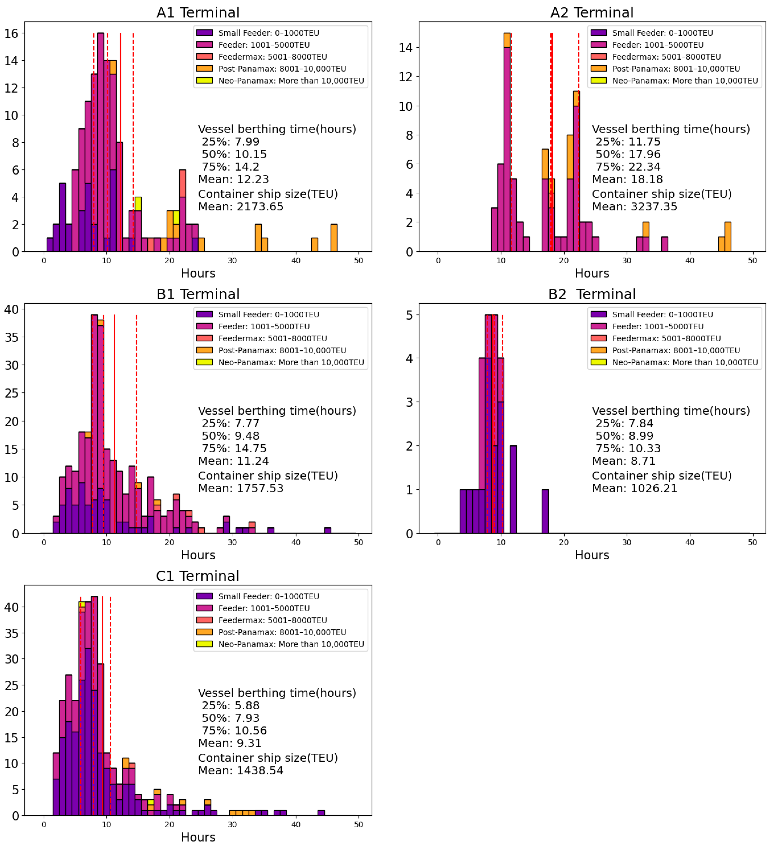
First, we tabulate the vessel berthing time (vessel turnaround time) for each terminal by extracting the time from vessel arrival to departure from AIS data, as shown in
Figure 1. Note that each terminal operates 24 h a day and 7 days a week, while truck gates open only during daytime hours except on Sundays. The figure shows that approximately 69% and 95% of containerships departed within 12 and 24 h of arrival, respectively. The terminal-level Pearson correlation coefficients between TEU capacity and turnaround time were as follows: A1: 0.768, A2: 0.489, B1: 0.286, B2: −0.087, and C1: 0.350. If all terminals were combined, the aggregated correlation coefficient was 0.513. The absence of a meaningful relationship at B2 Terminal can be explained by its small sample size and the narrow range of vessel sizes calling at the terminal, which limits the variability required for a stable correlation estimate.
These empirical patterns aligned with established findings in the literature [
22,
39,
40] regarding the relationship between vessel size and port time. For example, Malchow [
39], synthesizing operational data including Drewry’s calculations, showed that the largest containerships may require up to 70% more port-handling time than smaller ships. Similarly, the ITF-OECD [
40] provided concrete evidence that mega-ships (13,300 TEU or more) generally stayed in port about 20% longer than smaller vessels.
Taken together, our observed moderate positive correlation (overall r = 0.513) was broadly consistent with this body of research, although the strength of this relationship varied across terminals depending on equipment availability, berth allocation practices, and congestion levels. The strong correlations observed at A1 and A2 Terminals indicated terminals where vessel-size effects translate clearly into longer stays, while the weak or negative correlation at B2 Terminal exemplified conditions under which limited vessel-size variation or operational characteristics obscure the size–time relationship.
4.2. Time Distribution of Truck Arrival
Next, we analyze truck arrival times from the obtained TOS data for each terminal.
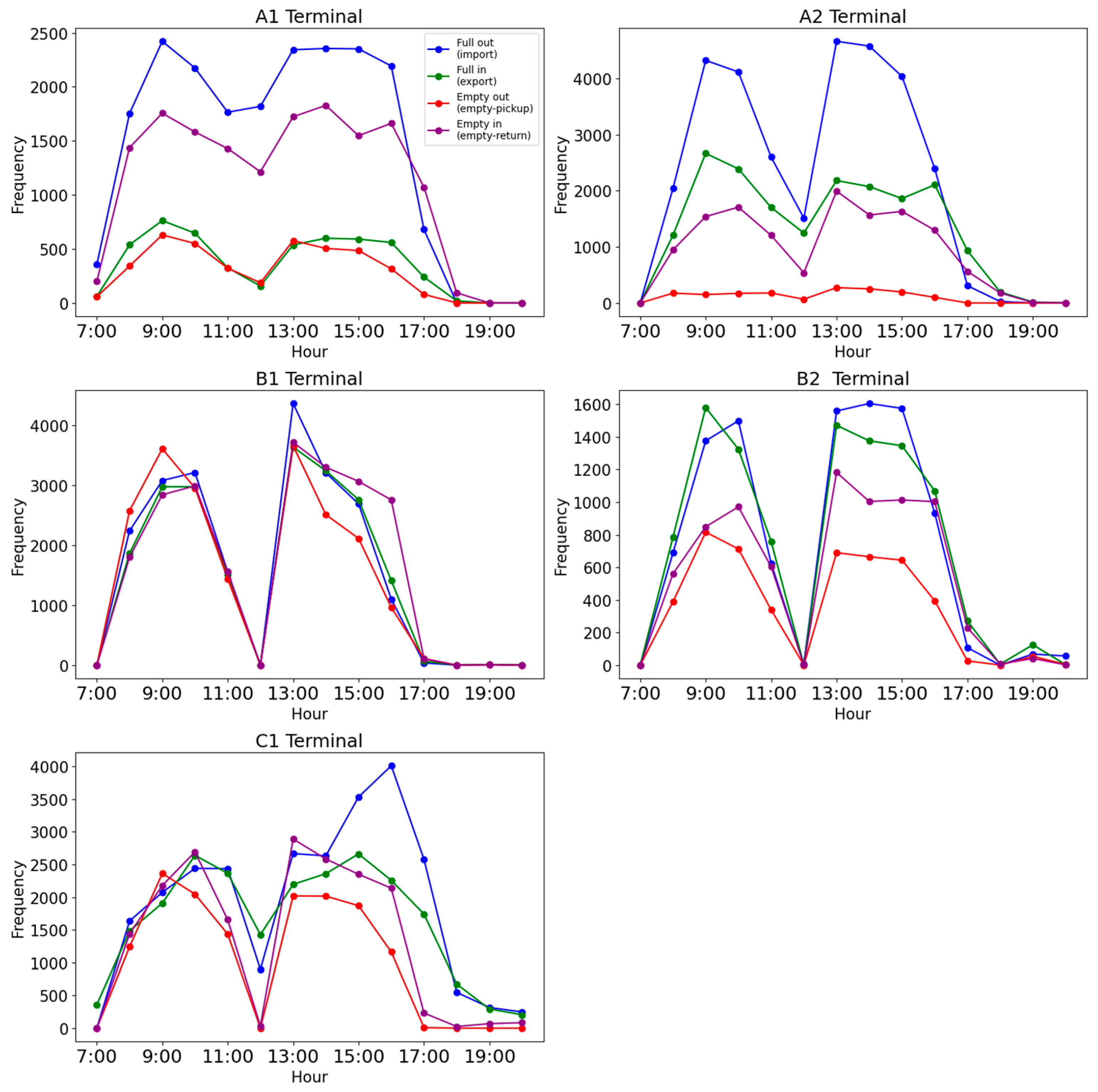
Figure 2 shows the time distribution of trucks arriving at each terminal by cargo type (full or empty and gate in or out). The time distribution is generally consistent across terminals in the daytime, with a break at noon and two peaks in the morning and afternoon, as observed in previous studies of Japanese container ports [
41].
In Port A, both terminals imported more full containers than they exported. At A1 Terminal, the number of empty gate-in containers was almost the same as full gate-out (i.e., import) containers, and that of empty gate-out containers was almost the same as full gate-in (i.e., export) containers, reflecting that almost all export and import containers were transported empty on their reverse trips, while there were significant differences between them at A2 Terminal. In addition, the noon break is characterized by a smaller valley at A1 Terminal compared to other terminals. In each terminal in ports B and C, the number of export and import containers was almost the same, while the balance between full (export and import) and empty containers differed between terminals—they were almost the same at B1 and C1 Terminals, but with more full containers than empty containers at B2 Terminal.
Overall, import containers tended to arrive in the morning, while export containers arrived in the afternoon at all terminals. Similarly, gate-out empty containers (i.e., reverse trips of export containers) tended to arrive in the morning, while gate-in empty containers (reverse trips of import containers) tended to arrive in the afternoon in most terminals. Chi-squared tests examined the relationship between cargo type (import or export) and arrival time (morning or afternoon) with a significant association (full containers: χ2(1) = 22.16; empty containers: χ2(1) = 665.56). Based on these findings, it was concluded that there is a statistically significant relationship between cargo type and delivery time.
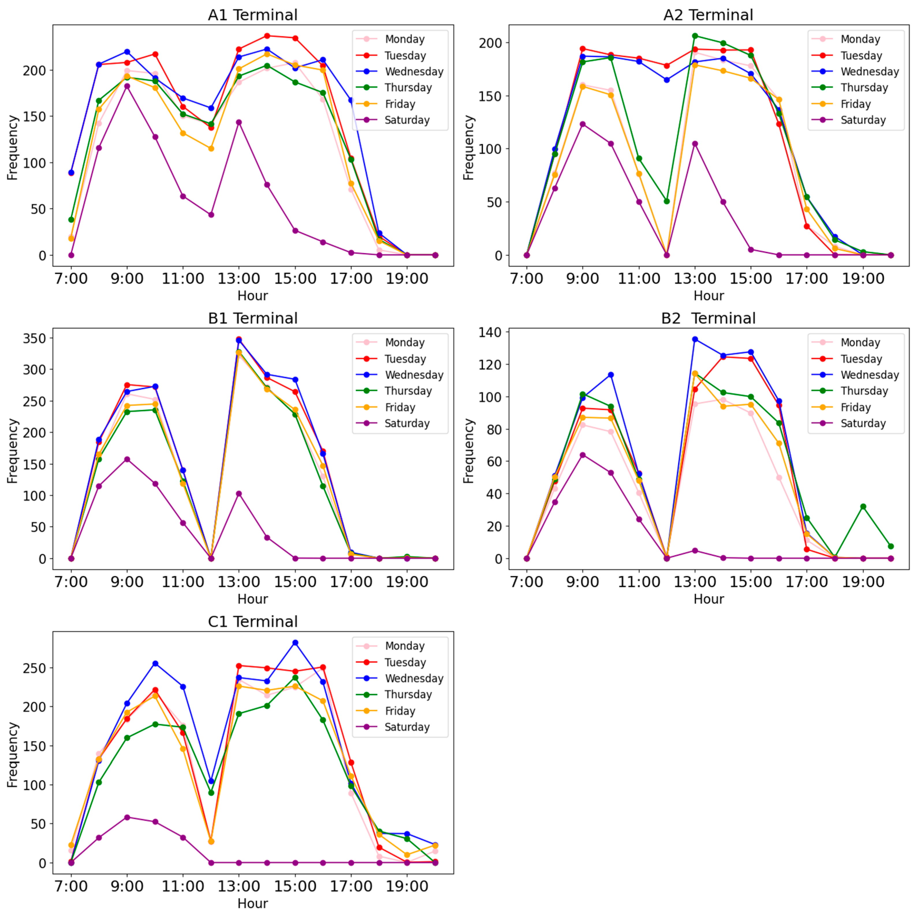
Figure 3 shows the distribution of truck arrival time by day of the week for each container terminal. All terminals accept trucks Monday through Saturday, with Saturday typically seeing lower truck volume. There were no significant differences in weekdays in most terminals, except for A2 Terminal, which had no lunch break on Tuesdays and Wednesdays.
4.3. Truck Turnaround Time
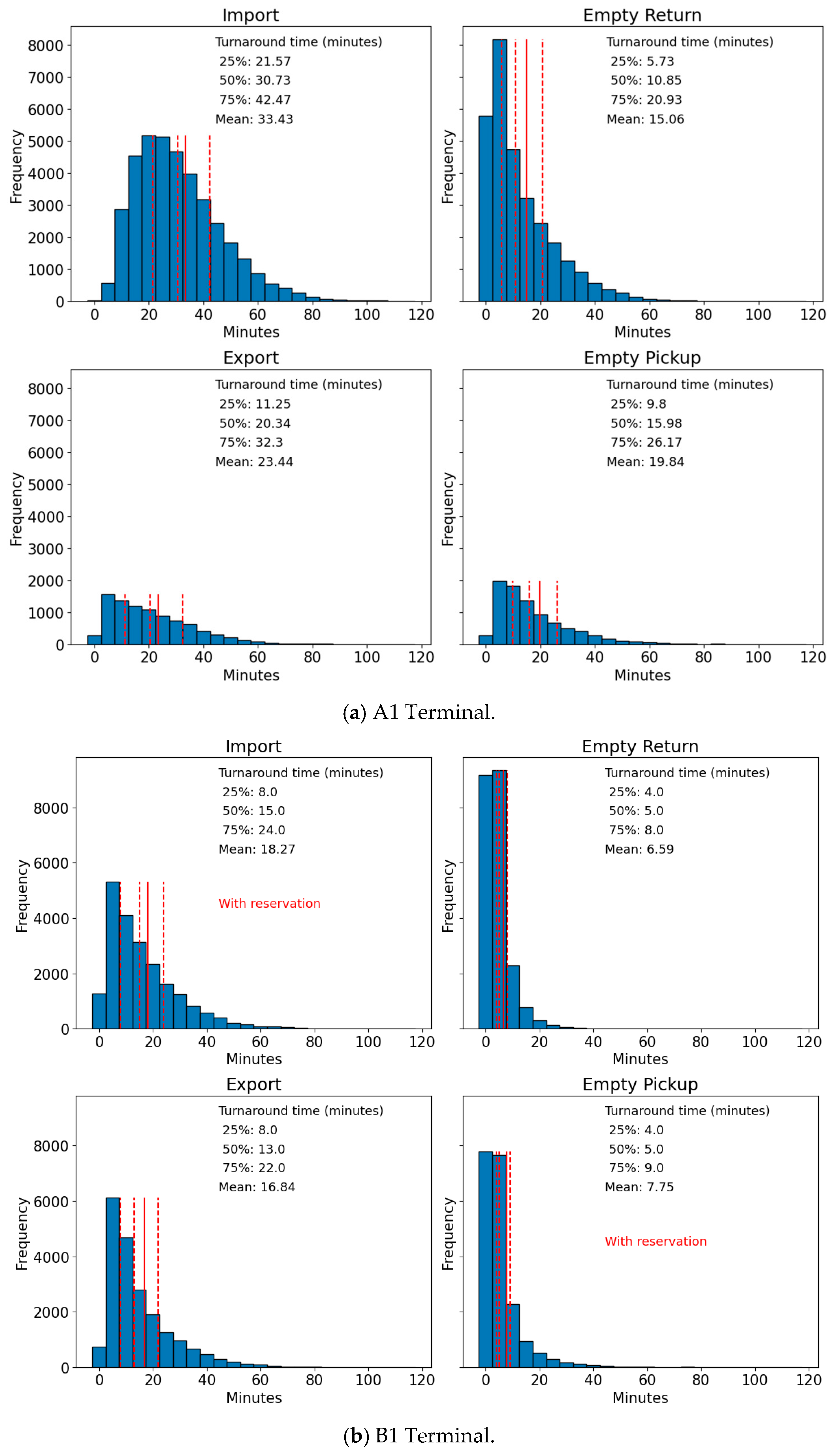
Subsequently, we analyze the turnaround time for inbound and outbound trucks from gating in to gating out, which can be estimated at A1, B1, and B2 Terminals. Due to data availability constraints, the definition of turnaround time differs by truck movement direction. For outbound trucks (i.e., import and empty-out containers), the turnaround time is measured strictly as the duration from gate-in to gate-out. In contrast, for inbound trucks (i.e., export and empty-in containers), the observed time represents the duration from gate-in to completion of unloading. Notably, each record is linked with only one cargo type, and all outbound containers at B1 Terminal used the reservation system.
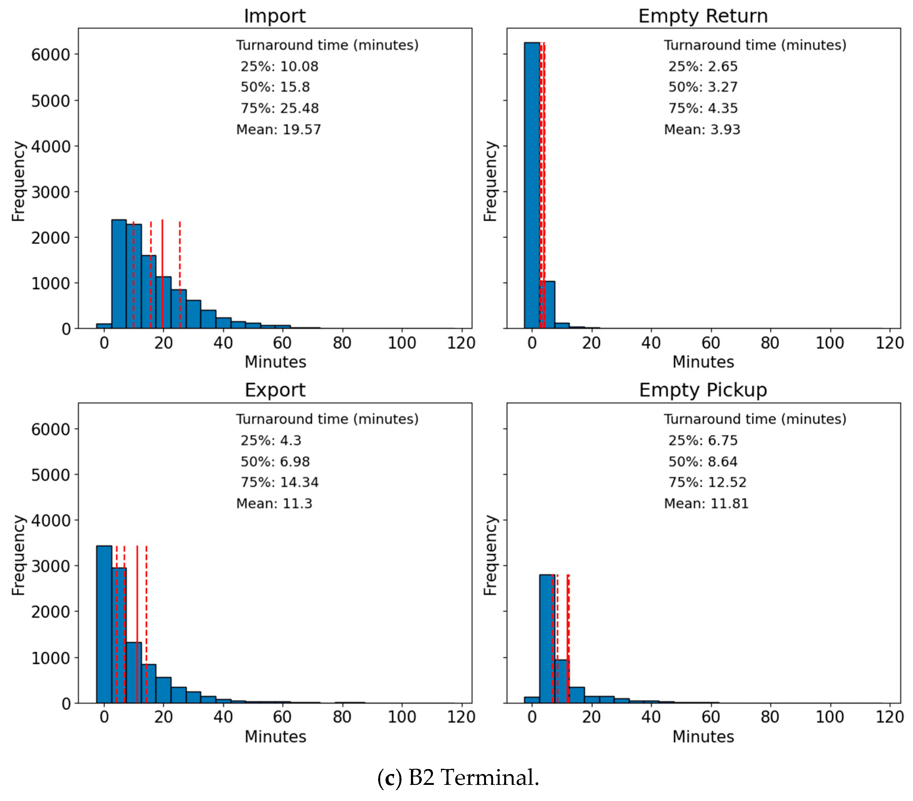
Figure 4 shows the turnaround times by cargo type at each terminal. Across all terminals, the results indicate that the truck turnaround time for import containers was generally longer than empty pickups (empty-out), and that for exports containers was longer than empty returns (empty-in), while the absolute values (including average turnaround time) were different between terminals, which depend on their capacity and congestion level, shape, handling equipment, and cargo contents (including foreland and hinterland characteristics) [
9,
10]. If focusing on the difference between import and export containers, the truck turnaround time for import containers was apparently longer than that for export containers at A1 and B2 Terminals (33.4 and 19.6 min of average truck turnaround times, respectively, for import, while 23.4 and 11.3 min for export). These observations indicate that trucks often waited to be loaded in the yard if they carried out import containers, while they did not need to wait in the yard for unloading export containers, even considering that the time from completion of unloading in the yard to gating-out was not included for gate-in containers. In contrast, the truck turnaround times for import and export containers at B1 Terminal were almost similar (18.3 and 16.8 min, respectively). A similar trend can be observed for empty containers: the differences in truck turnaround time between empty-in and empty-pickup containers were larger at A1 and B2 Terminals than at B1 Terminal. These results may be partly attributed to the reservation system introduced at B1 Terminal for gating-in trucks, reducing the truck turnaround times by repositioning containers in the yard before trucks arrive. Another possible explanation is its balanced numbers of gate-in and gate-out trucks (i.e., relatively small shares of gate-out trucks), as discussed in
Section 4.2, even though the larger number of trucks per hour gating out than other terminals, leading to a decrease in the turnaround time for gate-out trucks by reducing the complexity of yard operations.
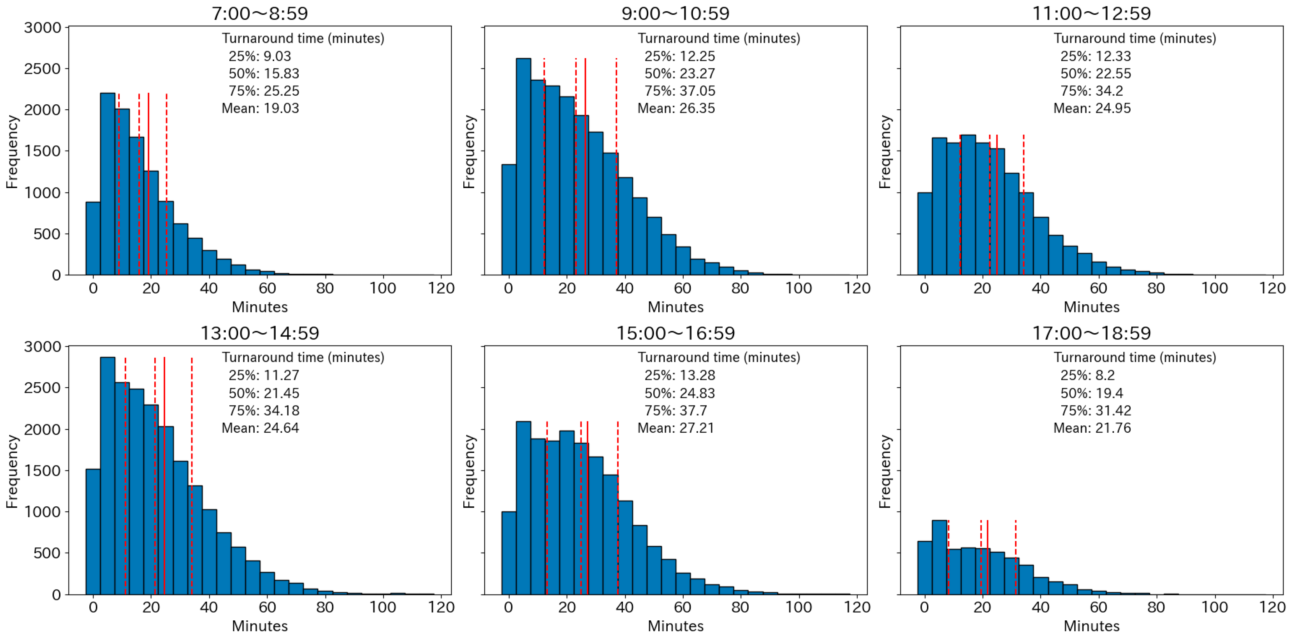
Figure 5 shows the distribution of truck turnaround times at A1 Terminal by time zone. Their average from 7 to 9 am was 19 min, more than 5 min shorter than in the other time zones. We also confirm there was no significant difference in the distribution, even at lunchtime. These observations were consistent with results at other terminals (B1 and B2 Terminals), shown in
Figure S1 in the
Supplemental Material, as well as our interview survey results with operators: yard operations for trucks accepted before the lunch break are completed before the break.
Next,
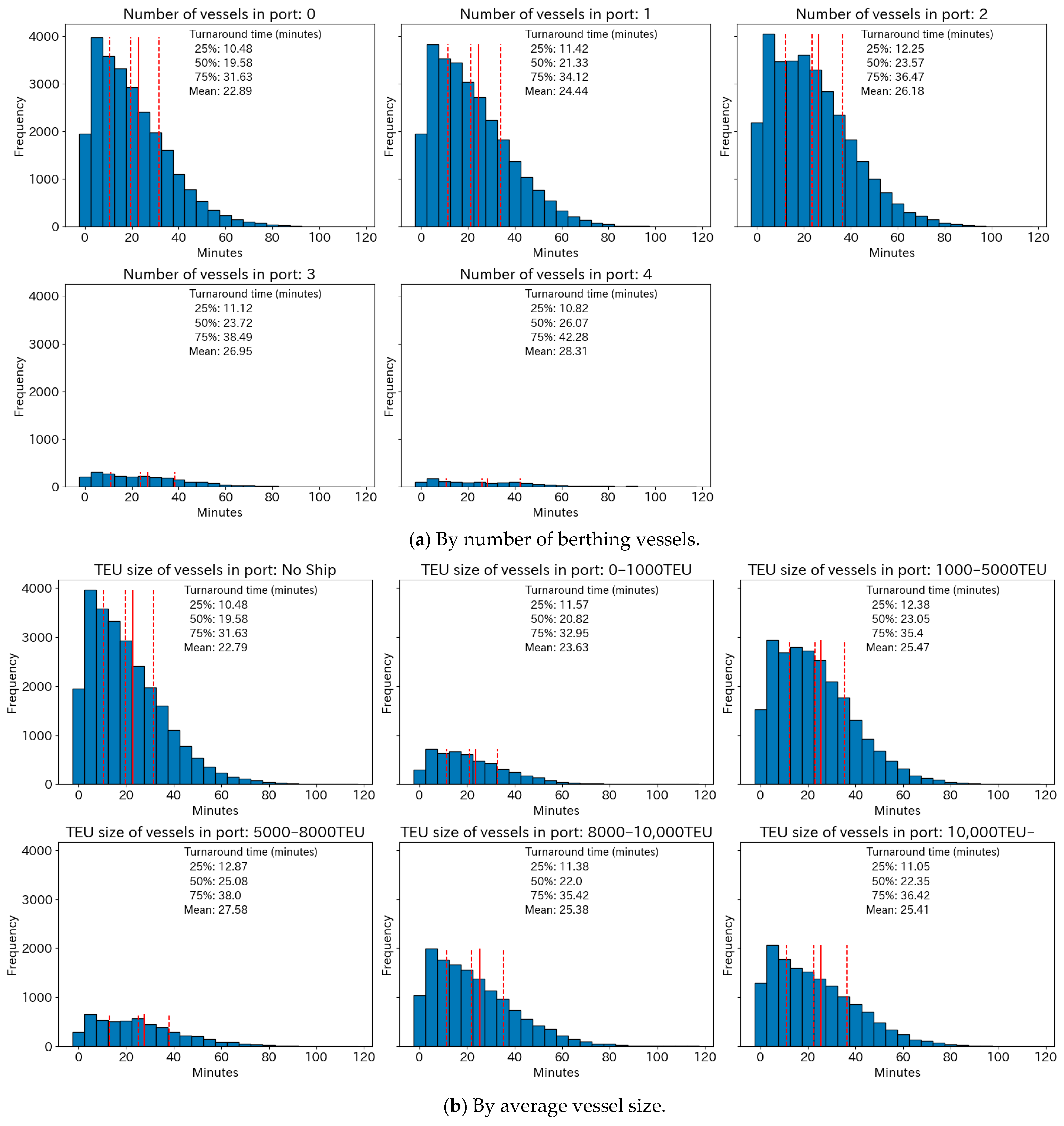
Figure 6a shows the distribution of truck turnaround times at A1 Terminal by the number of vessels calling, indicating that the average turnaround time was slightly longer if the number of vessels calling at the terminal increased. The same trend can be observed at B1 and B2 Terminals, as indicated in
Figure S2 in the
Supplemental Material. The average truck turnaround time, both with and without berthing vessels, was significantly different across terminals at the 1% significance level (t_value: −21.97). This is because the quayside operation is generally prioritized when the vessel calls, and trucks should wait in yard operations if a chassis comes from the quayside.
Figure 6b shows the distribution of truck turnaround times at A1 Terminal by average vessel size (those at B1 and B2 Terminals are shown in
Figure S3 in the
Supplemental Material). Unlike the number of berthing vessels shown in
Figure 6a, there was no tendency for the average truck turnaround time as the average vessel size increased if the vessel size was larger than 1000 TEU.
To identify the factors influencing truck turnaround times, we conducted a multiple regression analysis. The dependent variable is truck turnaround time, which is logarithmically transformed to reduce skewness and approximate normality because its distributions shown in
Figure 4,
Figure 5 and
Figure 6 are right-skewed with long tails. The independent variables include cargo types (empty or full, export or import, and dry or reefer); day of the week (weekday or Saturday); time (early morning: 7:00 to 8:59 am; morning: 9:00 to 11:59 am; midday: noon to 0:59 pm; afternoon: from 1:00 pm onward); and the number of vessels called at the terminal during the operation. We set empty gating-in containers to arrive early in the morning on weekdays as the reference.
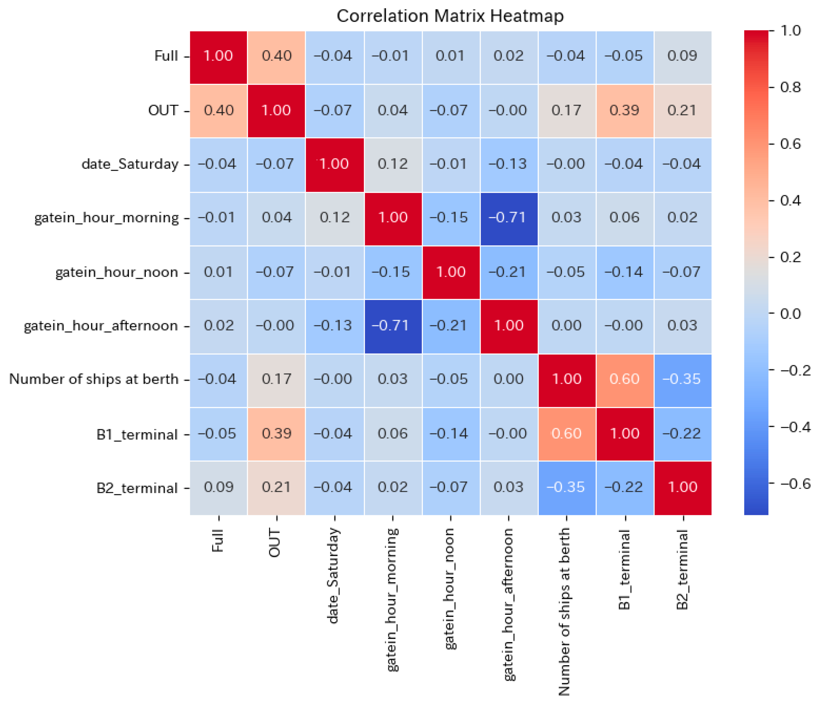
Figure 7 shows an example of a correlation matrix heatmap of dependent variables in all terminals, indicating no strong correlations between any dependent variables except for the strong negative correlation between different time zones (morning and afternoon). Notably, we also examined several more complicated models (e.g., LightGBM, Random Forest, Gaussian Regression, Lasso Regression, and Decision Tree Regressor). However, no significant differences relative to linear regression were observed; thus, we finally adopted the linear regression model for simplicity.
Table 3 presents the regression model estimation results for each terminal and for the combined data from all terminals. Overall, the multiple correlation coefficients are around 0.3–0.4, while most coefficients in the model are significant, indicating that truck turnaround times can be partly explained by the factors considered in this model. Among the model’s factors, the coefficients for full and gating-out containers are positive in each model, as discussed based on the observations in
Figure 4. Regarding the gate-in time, the coefficient in each time zone is positive in all models, indicating that truck turnaround time is fastest in the early morning, as shown in
Figure 5 for A1 Terminal. Lunchtime is the second fastest. The number of vessels calling at the terminal also has a positive effect on each model, as observed in
Figure 6a for A1 Terminal. However, the signs of the coefficients for Saturday operations and reefer containers differ by model: Saturday operations are faster than weekday operations because of lower congestion in some terminals, but slower in others because of a lack of available workers. The positive coefficient for Saturday estimated at A1 Terminal indicates longer truck turnaround times on Saturday because the proportion of the number of trucks arriving there on Saturdays relative to weekdays was higher than at other terminals, as shown in
Figure 3. The degree of congestion for reefer containers compared to dry containers also depends on their stocking capacities. Among all containers recorded in TOS data, the share of reefer containers at A1 and B2 Terminals was 9.5% and 10.9%, respectively, while the share of reefer area, calculated by satellite images, was 13.7% and 13.8%, respectively. This indicates less congestion in the reefer areas at A1 Terminal, resulting in a negative coefficient in
Table 3. Additionally, the model for all terminals yields results similar to those of the models developed for individual terminals, but it also shows that the difference in truck turnaround times between terminals is significant, as indicated by the t-values for the terminal dummy variables.
Notably, as indicated by the relatively small multiple correlation coefficients in these models, truck turnaround times also depend on other detailed factors not considered in the models, such as container positioning in the yard (especially for gating-out trucks), irregular congestion, and disruptions to vessel schedules. Although these factors mainly cause the longer-tailed distributions of truck turnaround time shown in
Figure 4,
Figure 5 and
Figure 6, our focus is on extracting more general factors that affect the mean turnaround time, as discussed earlier; therefore, these detailed factors are beyond the scope of this study.
4.4. Container Turnaround Time Within the Terminal
This subsection analyzes the terminal dwell time (turnaround time) of full containers. Since this requires that each container be linked to the vessel from which it is loaded or unloaded, the analysis targets A2, B1, and C1 Terminals. The vessel information is combined with AIS data using the vessel name and call sign from the TOS data in each terminal. Notably, empty containers are considered in the subsequent subsection because their vessel information is defined differently.
We consider two options for combining TOS and AIS data. The first option aims to increase container-vessel matching rates as much as possible, while the second focuses on matching accuracy. The details of the combining method are described below, by export and import.
Export (gate-in) full containers:
- -
Option 1: Identify the first vessel leaving the next day after a truck arrived at the terminal (which is a typical CY-cut time) with the vessel name or call sign.
- -
Option 2: Identify the vessel leaving after a truck arrived if the vessel called at the terminal once during a month after the truck’s arrival.
Import (gate-out) full containers:
- -
Option 1: Identify the last vessel arriving the previous day before a truck arrived at the terminal.
- -
Option 2: Identify the vessel arriving before a truck arrives if the vessel called at the terminal once during a month before the truck’s arrival.
Table 4 summarizes the estimated matching rates for both options applying to each terminal. The matching rates for Option 1 are over 90%, while those for Option 2 are around 50–70%. In the following analysis, we adopt Option 2 for prioritizing matching accuracy, even though the matching rates are lower. Notably, the matching rates for long-haul shipping containers, as defined later, were 100% for both export and import, even for Option 2.
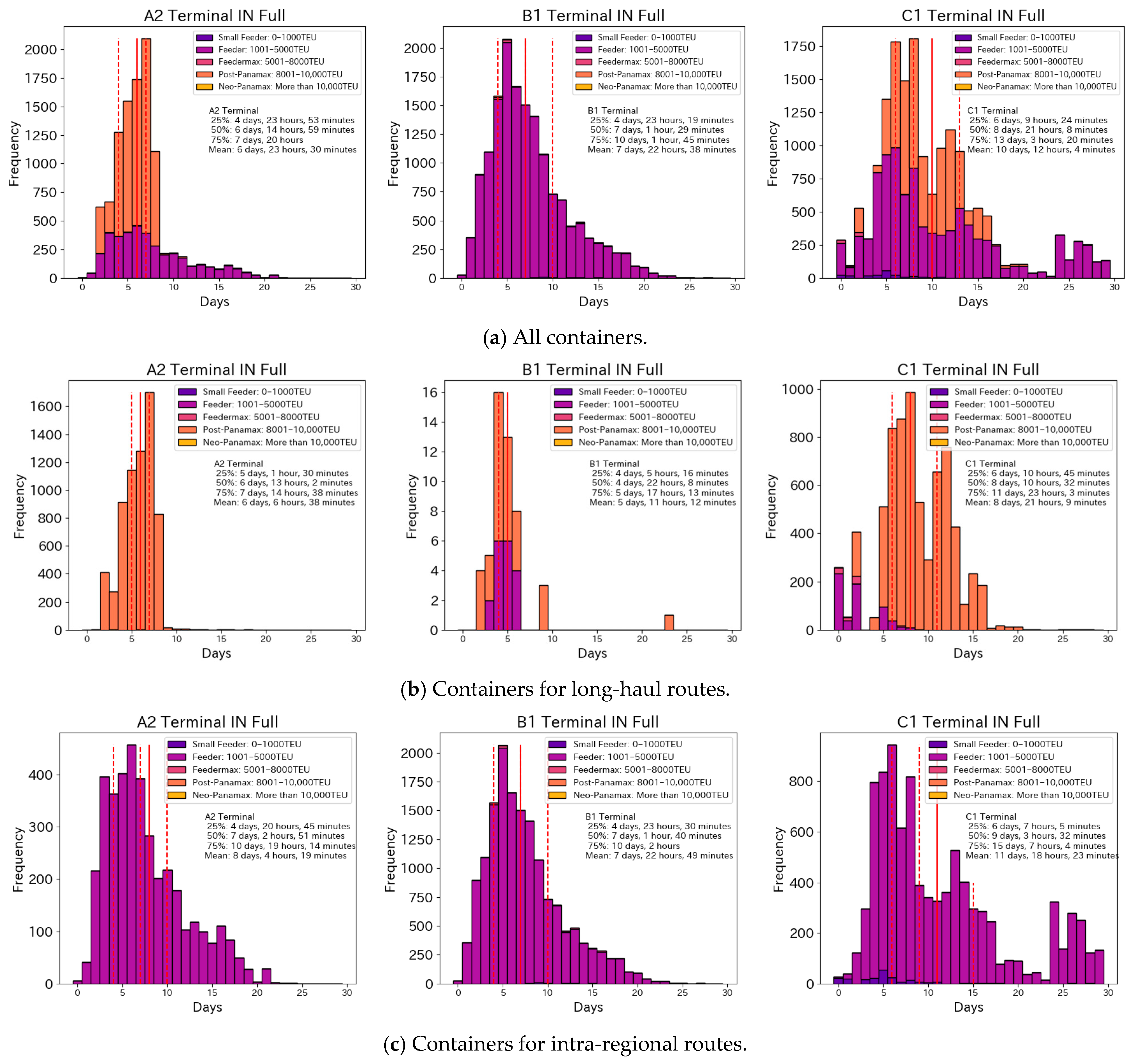
Figure 8a shows the distribution of turnaround times (colored by vessel size) for all export containers from the gating in of a truck to the departure time of the vessel at each terminal. At all terminals, the turnaround time was less than 48 h (2 days) for only a few containers. The turnaround time at A2 Terminal was the shortest, with very few containers remaining for more than one week, especially on the largest containerships, while the distribution at C1 Terminal shows two peaks at 6 to 8th and 12th days. These distributions were considered to be affected by CY-open time, which is the earliest time before the vessel departure and is normally set at one or two weeks before the departure.
Figure 8b,c show the turnaround time distribution for long-haul (including Europe, North, Central, and South America, and Africa) and intra-regional containers, respectively. Notably, the shipping route information is provided by the MDS data, and very few containers were transported on long-haul routes at B1 Terminal. They indicate that the turnaround times for export containers were longer-tailed on intra-regional routes in all terminals than on long-haul routes, suggesting that the duration from CY-open to CY-cut tended to be shorter on long-haul routes. The average turnaround time for intra-regional routes for each terminal was significantly longer at the 1% significance level (t_value: 26.03, 5.82, and 32.39 for each terminal).
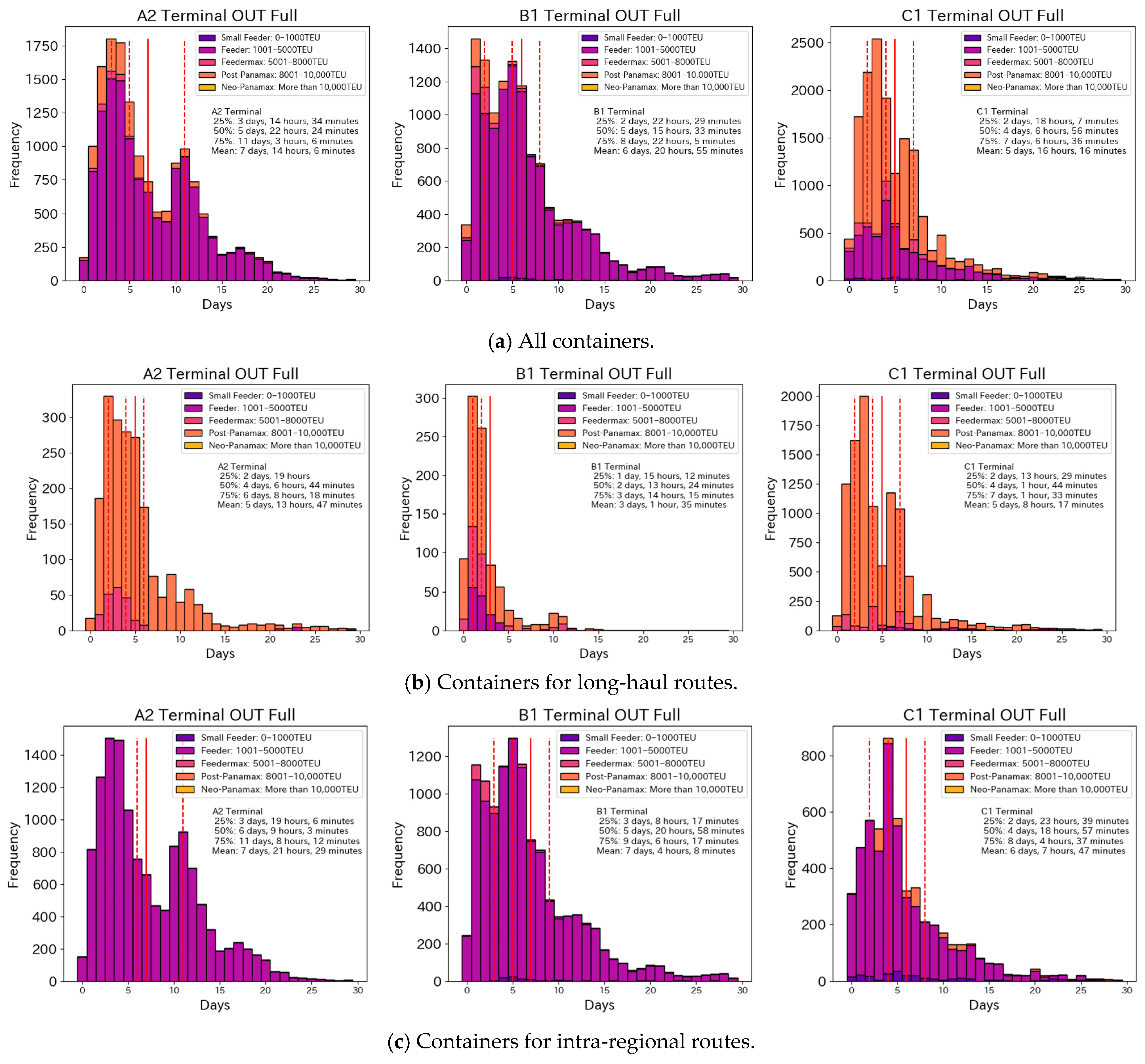
Figure 9a shows the distributions of turnaround times for all import containers from vessel arrival to truck gating-out at each container terminal. As with export containers, we find that turnaround time was less than 24 h (1 day) for only a few containers, reflecting the time required for import procedures. Since free time (the period during which the additional storage fee is not charged after vessel arrival) is generally set at seven days at each terminal, the majority of import containers were gated out within seven days of vessel arrival at each terminal, while some remained beyond free time. Because of the free time period, the average turnaround time for import containers was shorter than that for export containers. The exception was A2 Terminal, mainly because of seasonal differences; as shown in
Table 1, its data acquisition period was different (May and June), which included a Japanese holiday week in early May; thus, free time was considered extended during the holiday week. Therefore, its turnaround time distribution had two peaks.
Figure 9b,c show the turnaround time distribution for import containers on long-haul and intra-regional routes, respectively. The general trends in the results that container turnaround times were significantly longer for intra-regional routes at all terminals than for long-haul routes were similar to those of export containers at the 1% significance level (t_value: 19.14, 43.88, and 10.88 for each terminal), although a few import containers were transported on long-haul routes at A2 Terminal, different from the case of exports. This result indicates that intra-regional import containers tended to remain in the yard longer than long-haul import containers, even after free time ended. Additionally, even within free time, the peak turnaround times for intra-regional containers (three to five days) were longer than those for long-haul containers (one to three days). These observations indicate that the value of time for intra-regional import containers was smaller than that for long-haul import containers and that they tended to use the terminal as a substitute warehouse.
4.5. Container Turnaround Time Outside the Terminal
This subsection focuses on the container turnaround times outside the terminal, which is defined as the time from when the container left the terminal as an empty container to when it was delivered to the terminal as a full export container after vanning, or the time from when the container left the terminal as a full import container to when it was returned to the terminal as an empty container after devanning. We analyze A2 and B2 Terminals in this subsection because of data availability.
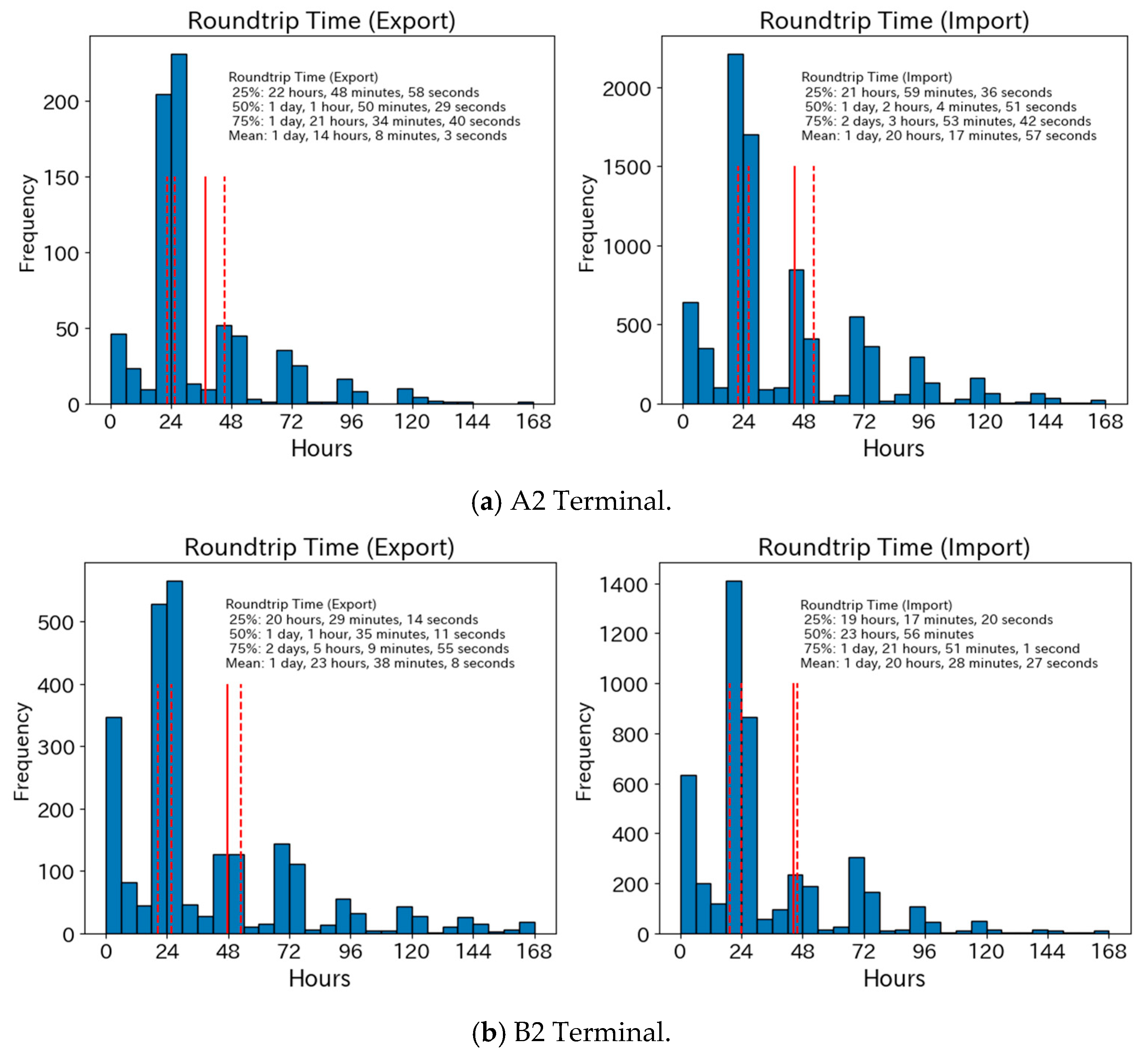
Figure 10 shows histograms of the turnaround time for A2 and B2 Terminals, respectively. While more containers returned to B2 Terminal within less than 6 h, compared to A2 Terminal, several common observations were noted. First, the turnaround time for export containers peaked at 24–30 h, while that for import containers peaked at 16–24 h. Peaks occur every 24 h because the terminal gates open during the daytime, and a very few containers were returned beyond 168 h (one week). Moreover, no significant difference in the container turnaround time distribution outside the terminal was observed between long-haul and intra-regional containers at A2 Terminal, where both values can be estimated, for both export and import.
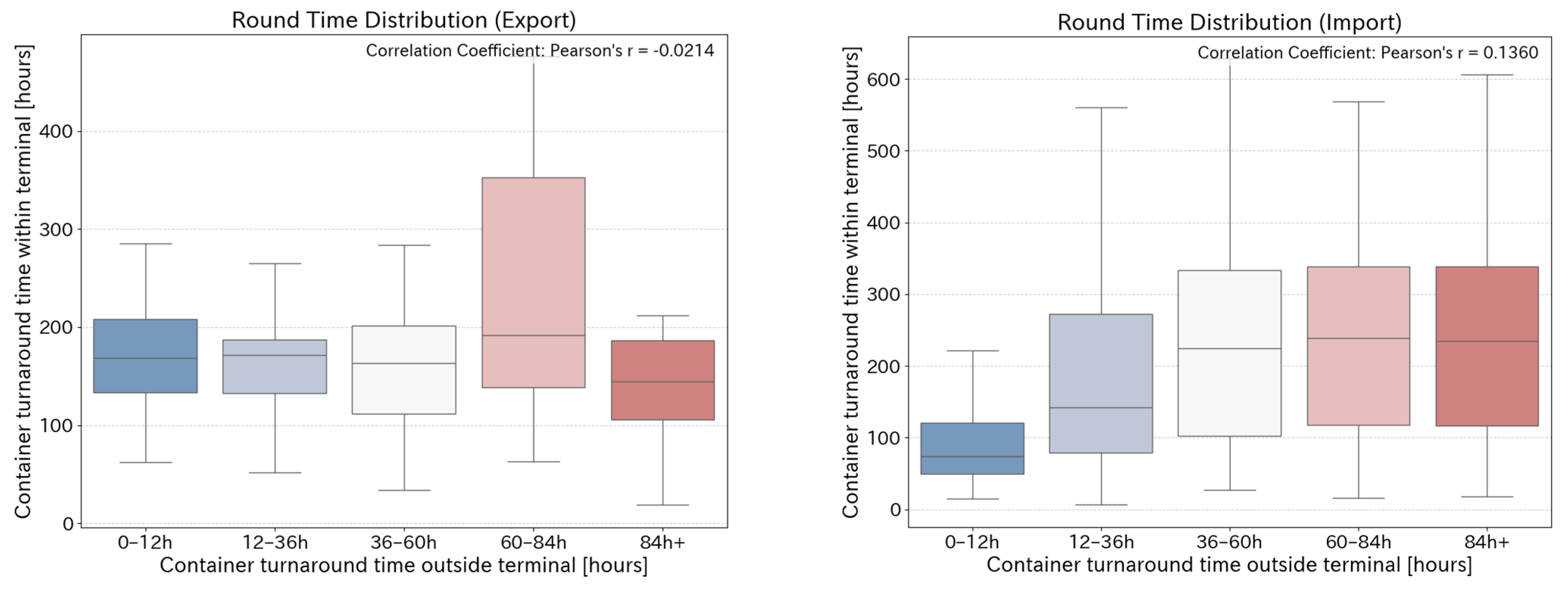
Additionally, we examine the relationship between container turnaround times within and outside the terminal at A2 Terminal, as shown in
Figure 11. Although no significant correlations were observed between them (−0.0214 and 0.136, respectively), different weak relationships were observed for exports and imports. For export containers, a weak negative relationship (trade-off) was observed, except for those that stayed outside the terminal for 60 to 84 h, suggesting that export containers waited for a vessel on board at the terminal or at the cargo origin point, such as factories. The exception for containers with a 60 to 84 h turnaround time outside the terminal can be explained by the fact that they stayed at the cargo origin point over the weekend because around two-thirds of them arrived at the terminal on Monday. Meanwhile, for import containers, a positive relationship was observed, especially for turnaround times of up to 60 h outside the terminal, indicating that containers quickly picked up from the terminal tended to return more quickly. This result reinforces our findings that there were different types of importing customers: fast- and slow-moving cargo.
5. Discussions
This study provides comprehensive empirical evidence on the operational patterns and efficiency determinants in container terminal operations, focusing on vessel, truck, and container turnaround times. Our analysis reveals several key insights with important implications for theory, practice, and policy.
5.1. Theoretical and Practical Implications
Regarding vessel turnaround time at major Japanese container terminals, our findings contribute to the comparative literature on port efficiency. It tended to be longer for larger vessels, as observed at terminals in other countries reported in other studies. However, this study reveals a unique “efficiency pressure” in the Japanese context. Due to the relatively small number of loaded and discharged containers per vessel in Japanese ports, they are facing the risk of being skipped by shipping companies. Therefore, effective and prioritized cargo handling to/from vessels is strongly required, and vessel turnaround time tends to be shorter: the majority of vessels left within 10 to 12 h, especially for smaller vessels, and most vessels left within 24 h. This result corroborates the findings of Malchow [
39], who synthesized operational data to show that the largest containerships can require up to 70% more handling time than smaller ones, and those of ITF-OECD [
40]. Unlike the major transshipment hubs discussed in those studies, our data suggest that, because Japanese terminals function increasingly as feeder or destination ports rather than primary hubs, maintaining shorter turnaround times is not just an operational goal but a commercial necessity to prevent service loops from bypassing them entirely.
The analyses on truck and container turnaround times further refine theoretical assumptions regarding terminal bottlenecks. Truck turnaround times were significantly affected by cargo type (import, export, empty-in, and empty-out) and terminals, among other factors (e.g., container positioning in the yard, irregular congestion, and vessel-schedule disruptions). The differences observed by cargo type suggest that the average truck turnaround time at the terminal with a large share of import containers will be longer, and thus, effective solutions, such as a truck appointment system and free-time control, are more necessary. While previous studies, such as Sun et al. [
33], used data-driven analysis to identify a non-linear relationship between truck volumes and operational time, demonstrating that optimized appointment quotas can effectively mitigate terminal congestion and enhance port sustainability, our breakdown by cargo type offers a more nuanced insight: generic appointment slots are insufficient. Instead, our results reveal that bottlenecks are structurally linked to the “imbalanced” arrival patterns of import versus export trucks. By quantifying such an imbalance risk between import and export flows, our study provides the empirical parameters needed for robust optimization models that account for operational uncertainty. Additionally, significant differences in truck turnaround times across terminals indicate that optimal solutions may vary by terminal, depending on terminal area, shape, and layout, as well as cargo characteristics (e.g., share of each cargo type). Moreover, truck turnaround times increased with the increased number of vessel calls at a terminal, suggesting capacity constraints in shared facilities, such as yard cranes, during high-activity periods, as quayside operations are prioritized. This finding supports the theoretical argument for integrated optimization under uncertainty, such as presented by Wang et al. [
28], suggesting that treating port operations as deterministic fails to capture the stochastic disruptions caused by arrival variability.
The analysis of turnaround times of full containers within terminals indicates that they were strongly affected by the CY-open time (for export containers) and free time (for import containers). Among them, intra-regional containers stayed longer than long-haul containers, reflecting their lower time value. In particular, controlling the timing of container pickup is difficult because some containers remain in terminals as substitute warehouses beyond free time, even if cargo owners must pay a penalty, which is a significant current challenge for congested terminals. This phenomenon extends Huynh’s [
36] findings, which demonstrated that increased container dwell time significantly constrains terminal throughput and reduces rehandling productivity under various storage strategies. This study further reveals the specific economic driver behind such dwell patterns in the Japanese context. For intra-regional importers, the daily demurrage cost at the terminal is often lower than the marginal cost of warehousing and double-handling outside the port. Consequently, the “long dwell time” is a rational economic choice by cargo owners, implying that operational efficiency cannot be improved solely by terminal improvements but requires pricing intervention. By linking these dwell-time determinants with specific vessel and truck turnaround patterns, this research clarifies that the “storage-like” behavior is particularly prevalent among intra-regional cargo owners. This nuanced distinction complements Huynh’s broader observations on terminal productivity. Although raising charges beyond free time is considered difficult in Japanese terminals under business practices, some policies are necessary to encourage behavioral changes among cargo owners. The analysis of container turnaround times outside the terminal reveals that containers were moved on a daily basis because cargo owners operate during the daytime in principle. Additionally, there was a weak trade-off between the durations at the terminal and at the cargo origin point for cargo owners exporting containers, while there were variations between cargo owners importing containers: fast-moving importers quickly picking up and returning containers, and slow-moving importers sometimes using the terminal as a substitute warehouse. Such differences in cargo characteristics by cargo types and owners should be considered in detailed analyses of container terminal operations.
Furthermore, this study also demonstrates clear temporal patterns in terminal operations, with distinct morning and afternoon peaks in truck arrivals and systematic variations across different cargo types. Our chi-squared tests confirm a significant relationship between cargo type and arrival time: full import containers predominantly arrived in the morning, while full export containers arrived in the afternoon at these terminals. This temporal segregation, while organizationally convenient, creates operational pressures during peak periods. The observed patterns suggest that current terminal operations exhibit a predictable but suboptimal distribution of truck traffic, which may lead to congestion during peak hours. The distinct operational characteristics were also observed across different terminals. A2 Terminal’s elimination of lunch breaks on Tuesdays and Wednesdays represented an adaptive response to peak demand, while C1 Terminal’s evening time operations demonstrated the potential for extended operating hours. The balanced distribution of export- and import-full containers in Ports B and C, contrasting with Port A’s import-heavy operations, suggests different optimal strategies may be needed for different port profiles.
5.2. Policy Recommendations
Based on these empirical findings and the regression results, we propose several detailed policy recommendations tailored to the distinct operational profiles of the terminals.
First, regarding truck arrival management, terminals should implement dynamic scheduling systems, including intelligent truck appointment systems, tailored to traffic characteristics. For high-volume gateway terminals (e.g., A1 and C1), where distinct morning import and afternoon export peaks were observed, intelligent truck appointment systems should strictly target these peak hours. Our regression model (
Table 3) indicated that truck turnaround times are significantly shorter in the early morning; therefore, leveling these peaks by shifting traffic to off-peak hours could theoretically reduce the congestion penalty identified in our model. The value for decision-makers lies not just in implementing a booking system, but in calibrating quota caps for “morning import pickups” to flatten the peaks identified in our analysis. This recommendation is consistent with the framework proposed by Lei and Jia [
30], who demonstrated that active “vessel demand shifting” and synchronization strategies are essential for mitigating congestion risks. Our results confirm that similar demand-smoothing strategies applied to landside truck flows can significantly reduce the probability of gate disruptions. In contrast, for regional terminals (e.g., B2) characterized by smaller feeder vessels, a more flexible booking system synchronized with feeder vessel schedules would be more effective than rigid time-slot allocation.
Second, regarding infrastructure and resources, optimization strategies should differ as well. Automated gate systems and dedicated lanes for empty containers are prioritized for busy terminals (e.g., A1) to mitigate the significant impact of vessel berthing on truck turnaround times. However, for terminals with lower throughput but specific labor constraints, operational standardization such as flexible break schedules—similar to A2 Terminal’s Tuesday–Wednesday model—is a more cost-effective solution, as our data showed this approach effectively smoothed the truck arrival distribution compared to other weekdays. For logistics decision-makers, these findings imply a shift from static to dynamic resource allocation. Specifically, terminal managers should decouple gate operating hours for empty containers from those for full containers to reduce interaction effects and implement differential pricing schemes that penalize “storage-like” behavior for intra-regional cargo during peak congestion seasons, rather than applying uniform storage fees year-round. This supports the argument by Liu et al. [
42] regarding the joint allocation of resources, emphasizing that matching labor availability to stochastic arrival patterns is key to reducing the “tail risk” of extreme waiting times, a finding our data confirms is often driven by rigid schedules such as lunch breaks.
Third, yard space allocation may be optimized through dynamic zoning based on the distinct container dwell-time patterns identified in
Section 4.4. Specifically, terminals handling a high proportion of intra-regional cargo (e.g., B1 and B2) should implement “long-stay zones” to accommodate the significantly longer dwell times caused by the “floating warehouse” behavior. Conversely, terminals serving primarily long-haul routes (e.g., A2) should focus on “rapid turnover zones” to maximize use.
Finally, information systems can be enhanced to deploy real-time tracking systems for both full and empty containers and implement predictive analytics using historical data to forecast peak periods. Integrated systems that connect vessel arrival data with truck appointment scheduling should be developed alongside mobile applications to provide real-time updates on terminal conditions and waiting times. Operational standardization and best practices should be prioritized. Flexible break schedules similar to A2 Terminal’s Tuesday–Wednesday model should be implemented during high-volume periods, as our data showed this approach effectively smoothed the truck arrival distribution compared to other weekdays. Terminal-specific performance metrics should be developed to account for different import–export balances. Furthermore, regulatory frameworks requiring terminals to maintain minimum handling speeds during vessel calls can also be considered, along with systematic reporting of key performance indicators for all terminals.
5.3. Limitations of the Study and Future Research Directions
Despite the contributions, this study is subject to certain limitations that point toward necessary future work. First, regarding data availability, our analysis was restricted to two months and to specific terminals. The datasets used in this study were collected from different years and months, which may introduce potential biases arising from seasonal patterns, the COVID-19 pandemic, and changes in terminal operational practices. This study focuses on short-term operational indicators, which are primarily influenced by terminal-level operational rules and capacity constraints, rather than annual demand cycles. However, the impacts of long-term indicators should not be negligible; thus, future research using longer and continuous time-series data would enable a more detailed assessment of seasonal and structural changes in terminal operations.
Second, regarding matching accuracy, while we successfully created a composite database, the physical linkage between TOS and AIS data encountered technical challenges. These constraints highlight the need for more standardized data protocols to enable broader cross-terminal comparisons. In addition, if TOS data with many time points are available across all terminals, time-series change analysis could provide more insightful implications, especially for comparing before and after introducing the CONPAS. In this context, combining TOS data with detailed movement data for container semi-trailers—extracted from the ETC 2.0 [
43]—could enhance the scope of analysis by including information on customer locations and type (e.g., factory, warehouse, and depot).
Most notably, building upon the operational parameters and bottlenecks identified in this study, future research should develop a discrete-event simulation or optimization model to test the proposed recommendations quantitatively. Specifically, quantifying the decrease in truck turnaround time under the proposed dynamic scheduling system will be a critical next step. A quantitative assessment of the impact of dynamic pricing on truck arrival patterns would provide valuable insights for policy refinement. Analysis of the relationship between vessel size and terminal efficiency across different ports could inform infrastructure development decisions. Investigating empty-container logistics optimization strategies would address a significant operational challenge. Finally, studying the environmental impact of current truck arrival patterns could identify opportunities for sustainability improvements. Future studies could adopt a sustainable supply chain framework, such as that proposed by Jafarian et al. [
44], to quantify trade-offs between reduced gate waiting times and carbon emissions, thereby linking operational efficiency directly to environmental risk management.