Accelerated Benders’ Decomposition for Integrated Forward/Reverse Logistics Network Design under Uncertainty

Abstract

In this paper, a two-stage stochastic programming modelling is proposed, to design a multi-period, multistage, and single-commodity integrated forward/reverse logistics network design problem under uncertainty. The problem involved both strategic and tactical decision levels. The first stage dealt with strategic decisions, which are the number, capacity, and location of forward and reverse facilities. In the second stage, tactical decisions, such as base stock level as an inventory policy, were determined. The generic introduced model consisted of suppliers, manufactures, and distribution centers in forward logistic and collection centers, remanufactures, redistribution, and disposal centers in reverse logistic. The strength of the proposed model is its applicability to various industries. The problem was formulated as a mixed-integer linear programming model and was solved by using Benders’ Decomposition (BD) approach. In order to accelerate the Benders’ decomposition, a number of valid inequalities were added to the master problem. The proposed accelerated BD was evaluated through small-, medium-, and large-sized test problems. Numerical results confirmed that the proposed solution algorithm improved the convergence of BD lower bound and the upper bound, enabling to reach an acceptable optimality gap in a convenient time.

1. Introduction

The main purpose of supply chain management (SCM) is to integrate entities including suppliers, manufacturers, distribution centers, and retailers, in order to acquire raw materials, transform raw materials to finished products, and distribute products to customers in an efficient way [1]. Achieving success in supply chain management involves several decisions relating to flow of information, products, and funds. The above-mentioned decisions fall into three levels: supply chain design, planning, and operations. In general, a Supply Chain Network Design (SCND) problem includes long-term decisions (strategic level), such as facility location, number, capacity level, and technology selection; mid-term decisions (tactical level), which usually contain the production quantity and the volume of transportation between entities; and finally short-term decisions (operational level) where all material flows are scheduled, based on decisions made in the two other levels [2].

Over the last decade, growing environmental awareness [3], social responsibility [4] and strict governmental regulations have changed the traditional management of supply chains, by showcasing the importance of integrating sustainable efforts to current management practices [5,6]. Sustainability efforts can be embedded from the first stages of product design and manufacturing to the recovery processes of product end-of-life stage [7]. Reverse Logistics (RL) is generally considered as the activities associated with returned products, such as collection, recovery, remanufacturing, refurbishing, and disposal of used or malfunctioned products [8]. In fact RL can be seen as part of sustainable development by ensuring the fact that “the society uses and reuses all the value which has been put into the product” [9].

The ways that organizations handle RL, in particular, product returns, depends on the nature of their products [10]. A study has shown that the chance of a sold product being returned is between 3 to 50, percent based on the industry [11,12]. For instance, the average return rate for the electronics industry is 8.5% and for the apparel and fashion industry it is 19.4%. The reason that RL is probably the most neglected section in supply chain practices [11] is the difficulties that come along with it. In comparison with forward supply chains that have uncertainties in customer demand, price [13] and resource capacity levels, RL operations are confronted with a higher degree of uncertainty, such as collection rates, availability of recycled production inputs, disposal, and recycling rates [14]. Greater uncertainty for forecasting returned products, many-to-one products movements [15] and associated transportation costs, due to lack of planning in transportation modes [16], as well as pricing of refurbished products [17,18,19,20,21] are examples of challenges related to RL.

Some RL networks only deal with backward products flows, originating from customers or buyers to the collectors’ facilities. For instance, Kim, Kang [22] tackled the problem of backward food waste transportation from local collecting areas to the designated treatment facilities in South Korea. Ferri, Chaves [23] built a model to manage municipal solid waste by implementing selective collection and composting of organic materials in Brazil.

While some research focuses on the planning and operation of backward logistics, a more complex, yet prevalent, showcase is exploring the supply chains that simultaneously have forward and backward logistics operations, generally called closed-loop supply chains (CLSC). Remanufacturing of returned products is one of the main activities associated with CLSC that has been practiced successfully in many industries, such as the printing industry [24], the electronic industry [25] (e.g., cellphones, cameras, and computers [26]), and the automotive industry [27]. De Brito, Dekker [28] provided a comprehensive review of case studies that have practiced RL and CLSC activities.

Although there is a wealth of literature that has studied CLSC networks, most studies only consider one out of the many aspects of CLSCs [19]. New models need to be developed to help the manufacturer optimize the system in an integrated view [29,30]. The true value of the closed-loop supply chain networks can be fully gained, only if all aspects of a CLSC are optimized in a coordinated way. For this purpose, in this paper an integrated forward/reverse logistic network will be introduced where, in the forward direction, the raw materials for the manufactures are gained from different suppliers, i.e., whole sale contract, spot market, and recycled material. In the backward direction, returned products are transferred to collection centers for inspection and classification purposes. Based on the quality of the returned products, they can be conveyed to distribution centers for reselling the product, to remanufacturing plants for refurbishment processes, or to disposal centers for the end-of life cycle. The refurbished products are conveyed to customers by a second channel to distribution centers for second market customers.

In this paper, we first developed a Mixed Integer Linear Programming (MILP) model for a multi-period, single-product, and capacitated integrated forward/reverse logistic network design. The model is formulated with a two-stage stochastic programming approach, with stochastic demand and returned product quantity. In the first stage, the number, capacity, and location of collections, plants and distribution centers, along with raw material acquisition are determined. In the second stage, tactical decisions such as base stock level for inventory management of distribution centers, are determined. The model is solved with Benders’ Decomposition (BD) approach where valid inequalities are added to accelerate the solution approach.

In summary, the major contribution of this research is an integrated forward/reverse logistic network design, amenable for forward and reverse flow, so that medium-term and long-term decisions are made simultaneously. Two of such tactical (medium-term) decisions are: (1) An inventory policy for distribution centers, considering new, returned, and refurbished products. A risk pooling policy is further analyzed at distribution centers for effective response to uncertainties in demand for new and refurbished products. (2) A raw material stocks policy for manufacturers, in which plants can provide the raw material from recycled product, spot market or long-term contract with certain suppliers. Selecting an appropriate inventory level for each facility (distribution centers and manufacturers) from predetermined capacity levels, based on the pull/push hybrid mechanism, is important in real-life applications, which is addressed in our model. The model is solved by a two-stage stochastic programming model, with an accelerate BD, where some valid inequalities are added to the master problem equations, in order to avoid infeasibility of problem solution space.

The remainder of the paper is organized as follows. In the next section, a review of literature, pertaining to stochastic closed-loop supply chain is investigated. In Section 3, a mathematical formulation of the proposed CLSD design is presented. The solution method is introduced in Section 4, followed by an analysis of computational results in Section 5. Finally, in Section 6, we conclude by reviewing contributions of this research and offer some issues for future research.

2. Literature Review

In recent years, a number of reviewing articles have been published on supply chains and reverse logistics (e.g., [31,32]). A recent paper by Govindan, Fattahi [33] provided a review of studies for both SCND and RL under uncertainty. They classified the papers, based on the planning decisions, network structure, and paradigms related to supply chain management, and discussed the stochastic optimization techniques used to solve the SCND problems. One of the areas that has been further investigated is the impact of disruption in SCND. Authors have concluded that future supply chains should be designed robustly to allow effective responses to disruptions made by both humans and nature (e.g., floods, earthquakes, terrorist attacks, and economic crises) [34,35,36].

Prior to this study, Govindan, Soleimani [37] reviewed papers on RL and CLSC, published between 2007 to 2013, with further investigation of papers that took sustainability and green issues into account. Ackali et al. [38] presented a critical review on RL and Integrated Forward/Reverse Logistic Network (IFRLN) problems, and discussed the main characteristics of models and solution methods proposed in the literature. Chanintrakul et al. [39] reviewed open-loop (forward supply chain) and closed-loop supply chain models by considering the impact of uncertainty in recent research. They argued the fact that few research studies have dealt with demand and return uncertainties, in terms of quality and quantity, and tactical decisions should be resolved, along with strategic decisions, which previous research has not effectively investigated.

As the importance of RL has emerged in recent years, various conceptual, mathematical, and socio-economical models have been developed to assist the operation and management of RL (e.g., [40,41,42,43,44]). In the last decade, RL networks became globally large and complex and the necessity of mathematical models to be a good proxy of real-world problems became inevitable. Mathematical models should embed the future uncertainties or plausible sources of randomness, to showcase complexities of RL networks. Uncertainty has been addressed as a stochastic parameter that changes over time, for any decision level, including strategic and tactical level decisions. At the tactical level, there has been a great deal of research that has signified the importance of uncertainties in decisions pertaining to the distribution of products, raw material acquisition, and demand fulfilments [45,46]. At the strategic level, a number of researchers have used uncertainties in the facility location of SCND under uncertainty [47]. Snyder, Atan [35] further classified risks and uncertainties in SC as Yield uncertainty, capacity uncertainty, lead-time uncertainty and cost uncertainty, where the “boundaries among these forms of supply uncertainty are often blurry” [35]. Including each, or combining of multiple uncertainties, increases the complexity of supply chain modelling and planning. Demand for the products is one of the examples of uncertainties that much of the SCN design literature considers a known, simplified static, and deterministic demand [31]. It has been shown that product demand fluctuates over time, due to several reasons, such as seasonality and introduction of new products into the market. An example of demand uncertainty was shown by Listeş and Dekker [48], in the recycling and re-use of sand originating from demolition waste in The Netherlands. Similarly, product return quantity varies, based on the expected life-cycle of a product, customer satisfaction, and quality of a product. In a case study presented by Salema, Barbosa-Povoa [49] demand for new products and return of products was shown to be stochastic in an office document company in the Iberian market.

For an integrated forward/reverse logistic network design, one of the first stochastic models was presented by Listes [50] and later Listes et al. [48]. The model only considers one echelon forward network, combined with two echelon reverse networks. The uncertainty is handled in a stochastic formulation by means of discrete alternative scenarios. Matthew et al. [51] studied a network design problem for carpet recycling in the United States (US) where supply and demand parameters were stochastic. Later Salema et al. [49] extended Fleischmann’s model [52] to a capacitated multi-product stochastic CLSC, applied to an office document company in Spain.

Most articles in stochastic IFRLN literature are single-period (e.g., [53,54,55,56,57,58]). Lee et al. [59] introduced a multi-period, multi-product dynamic location and allocation model, under demand uncertainty. To solve the model, an integrated sampling Average Approximation (SAA) method, with a simulated annealing (SA) algorithm was developed.

The literature that studied stochastic IFRLN network design problems, considering inventory policies, are few. Lieckens et al. [60] extended a closed-loop supply Mixed-Integer Linear Programming (MILP) model, combined with queuing characteristics, using a G/G/m model, which increased dynamic aspects, like the lead time and inventory position of the basic model. Since combining RL with a queuing model intensifies the computational complexity of the model, they restricted it to a single-level, single-product network design problem that covered a single-period. The new MINLP was solved with the differential evolution technique (DE). El-Sayed et al. [61] proposed a MILP multi-period, multi-echelon forward and reverse logistic network design model under uncertainty. The problem was formulated to maximize the total expected profit under risk. To achieve a generic model of CLSC, the authors incurred various costs, such as transportation, materials, remanufacturing, recycling, disposal, non-utilized capacity, storage, shortage, recycling, and inventory holding cost.

Table 1. Modeling approach codes.

Category	Detail	Code	Category	Detail	Code
Model objectives	Cost minimization	CM	Features of model	Period
	Profit maximization	PM		Single-period	S
	Responsiveness	R		Multi-period	M
	Quality	Q		Facility capacity
	Other	OT		Un-capacitated	U
Features of model	Stochastic parameters			Capacitated	C
	Quantity of demand	D		Capacity expansion	CE
	Quantity of returns	R		Single sourcing	SS
	Quality of returns	RQ	Model	Mixed Integer Linear Programming	MILP
	Recovery rate	RR
	Recovery cost	RC		Mixed Integer Non-Linear Programming	MINLP
	Transportation cost	TC
	Lead time	LT	Decision variables of model	Inventory decisions	I
	Income	In		Facility capacity	Fc
	Other	OT		Demand satisfaction	D
	Product commodity			Transportation values	TV
	Single-commodity	S		Location/allocation	LA
	Multi-commodity	M		Transportation mode selection	TM
			Solution methodology	Technology selection	TS
				Exact solution method	EX
				Heuristic solution method	HE

and

Table 2. Summary of stochastic integrated forward/reverse logistic network design.

Ref.	Model Obj.	Stoch. Param.	Product Com.	Period	Facility Cap.	Model	D.V.	Sol. Method	Solution Approach
[50]	PM	R	S	S	C	MILP	TV, LA	EX	B&C
[51]	PM	D	M	M	C	MILP	TV, LA, Fc, TM	-- a	AIMMS
[48]	PM	R, In	M	S	C	MILP	TV, LA	-- a	CPLEX
[62]	PM	D, R	S	S	C	MILP	TV, LA, SS	EX	Integer L-Shape Method
[49]	CM	TC, D, R	M	S	C	MILP	TV, LA, D	-- a	CPLEX
[60]	PM	LT	S	S	C	MINLP	TV, LA, Fc, I	HE	Differential Evaluation (DE)
[59]	CM	D, R	M	M	C	MILP	TV, LA	HE	SAA with SA
[54]	CM, OT	TC, R, OT	M	S	C	MILP	TV, LA, TS	-- a	CPLEX10
[58]	CM	TC, D, R, RQ	S	S	C	MILP	TV, LA	-- a	LINGO
[55]	PM	D, R	S	S	C	MILP	TV, LA	-- a	CPLEX
[57]	CM	D, R	M	S	C	MILP	TV, LA	EX	SAA with CPLEX
[53]	CM	RQ	S	S		MILP	LA	EX	SAA
[63]	CM, R, Q	D, R, RC, OT	M	S	C, SS	MILP	TV, LA, Fc	-- a	Commercial Solver
[56]	CM	D, R	S	S	C	MILP	TV, LA	-- a	CPLEX
[61]	PM	D, R	S	M	C	MILP	TV, LA, I	-- a	XpressSp
[20]	PM	OT	M	S	C	MILP	TV, LA	-- a	CPLEX
[64]	CM	D, R, RQ	S	S	C	MILP	TV, LA	-- a	CPLEX/GAMS
[4]	PM	R, RQ	P	S	C	MILP	TV, LA	EX	SAA
[65]	PM	D, R, TC	S	M	C	MILP	TV, LA	EX	Accelerated BD
Our paper	CM	D, R	S	M	C	MILP	TV, LA, I	EX	Accelerated BD

^a Commercial solver packages are used or the solution method is not reported.

structure a systematic review of the literature for closed-loop supply chain and integrated forward/reverse logistic network design problem under uncertainty. Characteristics of networks are coded and demonstrated in Table 1 and the review of existing studies are presented in Table 2. As shown in Table 2, most of the papers are those that are single-period and single-product. A few papers solve their model with an exact optimization approach, where utilizing commercial solvers are more common.

In this paper, we will first develop a MILP model for a multi-period, single-product, and capacitated integrated forward/reverse logistic network design. Due to the uncertainty of various parameters in real problems, demand and return quantity of products are considered to be stochastic. The model will be formulated with a two-stage stochastic programming approach. When analyzing real-world problems, while a policy scenario examination is desired, two-stage stochastic programming can be utilized effectively, for the models in which system information is uncertain [55]. In the two-stage stochastic programming, first-stage decisions are made instantly without considering the future outcome of uncertainty, but in the second stage, decisions are delayed until uncertainty has been eliminated. Therefore, in the first stage of the proposed two-stage stochastic model, strategic decisions will be determined, which are the number, capacity, and location of collection, plants and distribution centers as well as the number of wholesale contracts. Tactical decisions will be made in the second stage (e.g., base stock level). We will utilize Latin Hypercube Sampling to make scenarios from input data by considering correlations between each market. The model will be solved with an accelerating Benders’ Decomposition (BD) approach. Numerical tests investigate the power of accelerated BD in handling with uncertainty and solving the problem with an acceptable optimal gap.

3. Problem Definition

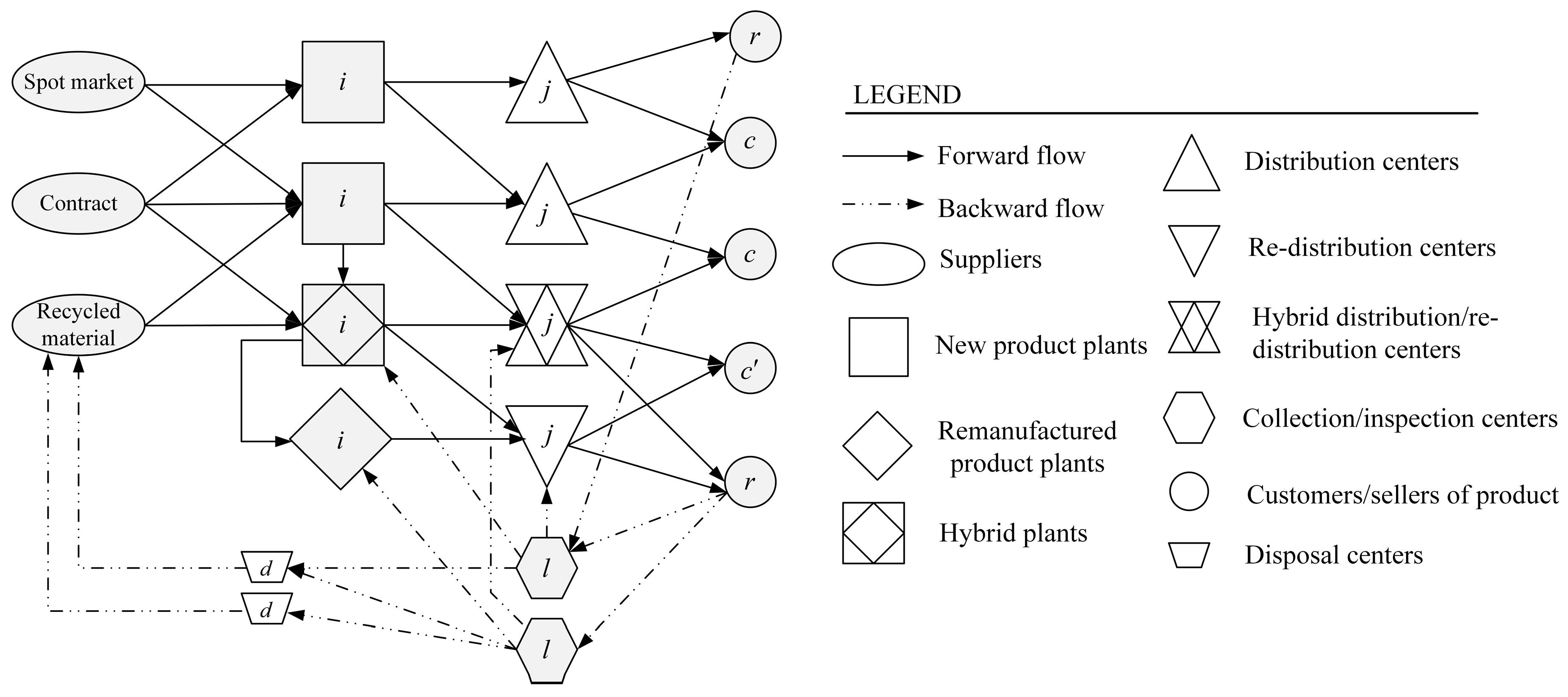
3.1. Model Description

The general structure of the proposed IFRLN is illustrated in Figure 1. In the forward direction, the new product is manufactured in plants from raw materials, provided from different suppliers, i.e., whole sale contract, spot market, and recycled materials. The product is conveyed from plants to customers through distribution centers within certain safety stock levels. In the backward direction, returned products are transferred from product sellers to collection centers for testing and inspecting. After classification, returned products are conveyed to distribution centers, remanufacturing plants, and disposal centers, depending on the amount of repair required. Remanufactured products are transferred to second market customers through certain distribution centers. This model is proposed with a generic nature, but it can encompass various industries, such as electronics, apparel, and automotive industries. In fact, the model is more appropriate for industries in which products can be highly remanufactured and sold in the second market as refurbished products.

The introduced model is a multi-stage, multi-period, capacitated, single commodity IFRLN under uncertainty. Our specifications for the model are listed below:

• The periodic review policy is used for the distribution centers and manufacturers, in which the inventory levels are reviewed at certain intervals and the appropriate orders are placed after each review. The inventory level of raw material should meet a specific amount in each period. The production and shipment from the manufacturers to the distribution centers takes place, to raise the inventory level of distribution centers to the base-stock level (S) at the beginning of each period. This concept is referred to as the push strategy in the related literature. On the other hand, customer demands are met with the inventory kept by the distribution centers. The customers only place orders to the distribution centers. This system is known as a pull-based system.
• A hybrid concept for production plants is considered. Due to the fact that locating manufacture and remanufacture plants in the same potential place will reduce fixed costs, we are interested in locating hybrid plants.
• In distribution centers, a risk pooling strategy is considered, where both new and remanufactured products are held simultaneously. The “risk-pooling” strategy is an efficient way of managing demand uncertainty, for which inventory needs to be centralized at distribution centers (DC’s) arriving at a convenient service level. Each DC uses a base stock level inventory policy to satisfy demands from retailers, as well as safety stock to cope with the variability of customer demand at retailers, to achieve “risk-pooling” benefits.
• As mentioned above, the inventory level of a raw material should meet a specific amount in each period. To this aim, raw material is provided through wholesale contracts, spot markets and recycled materials. A wholesale contract is a long term agreement with suppliers to convey a certain proportion of raw materials in the beginning of each period. If the amount of provided raw material from a wholesale contract and recycled material do not meet the base stock level in each period, the shortage of raw material is compensated for by buying from spot markets, but at a higher price.

To specify the study scope, assumptions and limitations in the proposed model, the formula is as follows.

• A single-product, multi-stage, multi-period supply chain network is given.
• We assume a finite set of facilities (i.e., manufacturers and distribution centers) should be opened.
• There is no limitation on the capacity of the material flow through the network.
• We are faced with uncertainty for the demand of the customers to the distribution centers and return of used products to collection centers.
• Transportation costs are linearly dependent on the distance between stages.
• Distribution centers and raw material stock at manufactures incur inventory holding costs at the end of each period.
• All of the returned products must be collected, but a shortage is allowed, to satisfy the demands of second market customers.
• Customers’ locations are known and fixed.

3.2. Model Formulation

According to Birge et al. [66], in a stochastic optimization model, decisions could be taken in two stages. In the first stage, strategic decisions are determined as here-and-now decisions, which should be made before the demand and return realization, and the tactical decisions should be made in the second stage as wait-and-see decisions. Moreover, the second stage in our model considers multi-periods, in which the tactical costs can be efficiently captured. This would be advantageous, specifically for those supply chain networks whose demands differ from one period to another period. The following notations are used for the mixed integer linear programming (MILP) of the proposed model:

Sets:
$I$	Set of potential manufacturer locations $i,i^{\prime }\in I$
$J$	Set of potential distribution center locations $j\in J$
$T$	Set of periods in planning horizon $t,k\in T$
$C$	Set of customers for new product $c\in C$
$C^{\prime }$	Set of customers for used product $c^{\prime }\in C^{\prime }$
$L$	Set of potential collection center locations $l\in L$
$D$	Set of disposal locations $d\in D$
$R$	Set of seller products $r\in R$
$S$	Set of scenarios $s\in S$
Parameters, constants, and coefficients:
Fixed costs:
${\mathrm{F}}_{\mathrm{i}}^{\mathrm{M}}$	Fixed cost of locating manufacturer at location i
${\mathrm{F}}_{\mathrm{i}}^{\mathrm{RM}}$	Fixed cost of locating remanufacturer at location i
${\mathrm{F}}_{\mathrm{j}}^{\mathrm{Dc}}$	Fixed cost of locating distribution center for new product at location j
${\mathrm{F}}_{\mathrm{j}}^{\mathrm{D}{\mathrm{c}}^{\prime }}$	Fixed cost of locating distribution center for used product at location j
${\mathrm{F}}_{\mathrm{l}}^{\mathrm{CL}}$	Fixed cost of locating collection center at location l
Capacity costs and saving costs:
${\mathrm{s}}_{\mathrm{i}}^{\mathrm{P}}$	Saving cost of locating a hybrid manufacture/ remanufacture facility at location i
${\mathrm{s}}_{\mathrm{j}}^{\mathrm{Dcs}}$	Saving cost of locating a hybrid distribution center facility at location j
${\mathrm{Vc}}_{\mathrm{i}}^{\mathrm{M}}$	Cost for capacity of manufacturer i per unit of product
${\mathrm{Vc}}_{\mathrm{i}}^{\mathrm{RM}}$	Cost for capacity of remanufacturer i per unit of product
${\mathrm{Vc}}_{\mathrm{j}}^{\mathrm{Dc}}$	Cost for capacity of distribution center j per unit of new product
${\mathrm{Vc}}_{\mathrm{j}}^{\mathrm{D}{\mathrm{c}}^{\prime }}$	Cost for capacity of distribution center j per unit of used product
${\mathrm{Vc}}_{\mathrm{l}}^{\mathrm{Cl}}$	Cost for capacity of collection center l per unit of returned product
Capacity of facilities:
${\mathrm{Cap}}_{\mathrm{i}}^{\mathrm{Max}-\mathrm{M}}$	Maximum available capacity of manufacturing at location i
${\mathrm{Cap}}_{\mathrm{i}}^{\mathrm{Max}-\mathrm{RM}}$	Maximum available capacity of remanufacturing at location i
${\mathrm{Cap}}_{\mathrm{j}}^{\mathrm{Max}-\mathrm{Dc}}$	Maximum available capacity for new products at distribution center j
${\mathrm{Cap}}_{\mathrm{j}}^{\mathrm{Max}-\mathrm{D}{\mathrm{c}}^{\prime }}$	Maximum available capacity for second hand products at distribution center j
${\mathrm{Cap}}_{\mathrm{l}}^{\mathrm{Max}-\mathrm{Cl}}$	Maximum available capacity of collection center at location l
${\mathrm{Cap}}_{\mathrm{i}}^{\mathrm{Max}-\mathrm{P}}$	Maximum available capacity for production facilities at location i
${\mathrm{Cap}}_{\mathrm{j}}^{\mathrm{Max}-\mathrm{Dcs}}$	Maximum available capacity for distributing center facilities at location j
Transportation costs:
${\mathrm{Tc}}_{\mathrm{ij}}^{\mathrm{M}-\mathrm{Dc}}$	Cost of transporting, per unit of product, between manufacturer p and distribution center j
${\mathrm{Tc}}_{\mathrm{jc}}^{\mathrm{Dc}-\mathrm{Cu}}$	Cost of transporting, per unit of new product, between distribution center j and customer c
${\mathrm{Tc}}_{\mathrm{j}{\mathrm{c}}^{\prime }}^{\mathrm{D}{\mathrm{c}}^{\prime }-\mathrm{C}{\mathrm{u}}^{\prime }}$	Cost of transporting, per unit of used product, between distribution center j and customer $c{u}^{\prime }$
${\mathrm{Tc}}_{\mathrm{rl}}^{\mathrm{Sr}-\mathrm{Cl}}$	Cost of transporting, per unit of product, between seller r and collection center l
${\mathrm{Tc}}_{\mathrm{ld}}^{\mathrm{Cl}-\mathrm{Di}}$	Cost of transporting, per unit of product, between collection center l and disposal d
${\mathrm{Tc}}_{\mathrm{di}}^{\mathrm{Di}-\mathrm{M}}$	Cost of transporting, per unit of recycled product, between disposal d and manufacturer i
${\mathrm{Tc}}_{\mathrm{lj}}^{\mathrm{Cl}-\mathrm{D}{\mathrm{c}}^{\prime }}$	Cost of transporting, per unit of product, between collection center l and distribution center j
${\mathrm{Tc}}_{\mathrm{li}}^{\mathrm{Cl}-\mathrm{M}}$	Cost of transporting, per unit of product, between collection center l and manufacturer i
${\mathrm{Tc}}_{\mathrm{i}{\mathrm{i}}^{\prime }}^{\mathrm{M}-\mathrm{Rm}}$	Cost of transporting, per unit of product, between manufacturer i and remanufacturer $i^{\prime }$
Inventory costs:
${\mathrm{Ic}}_{\mathrm{j}}^{\mathrm{Dc}}$	Cost of holding, per unit of inventory, in distribution center j
${\mathrm{Ic}}_{\mathrm{i}}^{\mathrm{M}}$	Cost of holding, per unit of inventory, in manufacturer i
Demand and return:
${\mathrm{D}}_{\mathrm{cst}}^{\mathrm{Cu}}$	Product demand of customer c in scenario s at period t
${\mathrm{Rs}}_{\mathrm{rts}}^{}$	Product returns of seller r in scenario s at period t
Other parameters:
${\mathrm{Pr}}_s$	Probability of scenario s
$\mathrm{BOM}$	The quantity of raw material needed for one unit of a product
${\mathrm{C}}_{\mathrm{sm}}$	Cost of buying raw material from spot market
Coefficients and ratios:
$\mathsf{\beta }$	Rate of raw material shipping from disposal center to raw material stock
$\mathsf{\lambda }$	Rate of new product shipping from manufacture centers to distribution centers
${\mathsf{\gamma }}_1$	Rate of product shipping from collection centers to distribution centers
${\mathsf{\gamma }}_2$	Rate of product shipping from collection centers to disposal centers
$\mathrm{M}$	A large number
${\mathrm{N}}_{\mathrm{t}}$	Number of periods
Decision variables:
Binary variables (relating to opening and locating facilities):
$x_i^M$	Binary variable equals 1 if a manufacturer is located at location i, 0 otherwise
$x_i^{RM}$	Binary variable equals 1 if a remanufacturer is located at location i, 0 otherwise
$y_j^{Dc}$	Binary variable equals 1 if a distribution center for a new product is located at location j, 0 otherwise
${y^{\prime }}_j^{Dc}$	Binary variable equals 1 if a distribution center for a used product is located at location j, 0 otherwise
$x_{{}_{i}i}^p$	Binary variable equals 1 if a manufacturer and remanufacturer are located at location i, 0 otherwise
$y_j^{Dcs}$	Binary variable equals 1 if a new product distribution center and used product distribution center are located at location j, 0 otherwise
$z_l^{Cl}$	Binary variable equals 1 if a collection center is located at location l, 0 otherwise
Continuous variables (relating to production and raw material acquisition):
$W_{}^C$	Quantity committed in wholesale contract
$r_{it}^M$	Quantity committed in contract to manufacturer i at period t
$s{m}_{ist}^M$	Quantity bought from a spot market for manufacturer i in scenario s at period t
$q{p}_{ist}^M$	Quantity of production from manufacturer i in scenario s at period t
Continuous variables (relating to capacity of facilities):
$c_i^M$	Capacity of manufacturer i
$c_i^{RM}$	Capacity of remanufacturer i
$c_j^{Dc}$	Capacity of distribution center j for new product
$c_j^{D{c}^{\prime }}$	Capacity of distribution center j for used product
$c_l^{Cl}$	Capacity of collection center l
Continuous variables (relating to inventory decisions):
$b_j^{Dc}$	Base-stock level of distribution center j at the beginning of each period
$b_i^M$	Base-stock level of manufacturer i at the beginning of each period
$in{v}_{ist}^M$	Inventory level of manufacturer i at the end of period t in scenario s
$in{v}_{jst}^{Dc}$	Inventory level of distribution center j for new products at the end of period t in scenario s
$in{v}_{jst}^{D{c}^{\prime }}$	Inventory level of distribution center j for second market products at the end of period t in scenario s
Continuous variables (relating to flows on network):
$f_{ijst}^{M-Dc}$	Flow of production from manufacturer i transported to distribution center j at period t in scenario s
$f_{dist}^{Di-M}$	Flow of material from disposal d transported to manufacturer i at period t in scenario s
$f_{ijst}^{RM-D{c}^{\prime }}$	Flow of remanufactured product from remanufacturer i transported to distribution center j in scenario s at period t
$f_{i{i}^{\prime }st}^{M-Rm}$	Flow of production from manufacturer i transported to remanufacturer $i^{\prime }$ in scenario s at period t
$f_{list}^{Cl-Rm}$	Flow of returned product from collection center l transported to remanufacturer i in scenario s at period t
$f_{ljst}^{Cl-D{c}^{\prime }}$	Flow of returned product from collection center l transported to distribution center j at period t in scenario s
$f_{ldst}^{Cl-Di}$	Flow of returned product from collection center l transported to disposal d at period t in scenario s
$f_{jcst}^{Dc-Cu}$	Flow of new product from distribution center j transported to customer c at period t in scenario s
$f_{j{c}^{\prime }st}^{Dc-C{u}^{\prime }}$	Flow of used product from distribution center l transported to customer $c^{\prime }$ at period t in scenario s
$f_{rlst}^{Sr-Cl}$	Flow of returned product from seller r transported to collection center l at period t in scenario s

It should be noted that the uncertain demand and return in our mathematical formulation is introduced by $\zeta$. ${\zeta }_S$ is a given realization of uncertain parameters and $E_{\zeta }$ represents the expected value with respect to $\zeta$.

According to Birge and Louveaux [66], the actual value of $\zeta$ becomes known in the second stage, in which recourse decisions can be calculated. Therefore, decisions related to the first stage are made by taking the future uncertain effects into account. These effects are measured by the recourse function, $Q\left(x,w,b\right)=E_{\zeta }\left(Q\left(x,w,b,{\zeta }^S\right)\right)$, where $Q\left(x,w,b\right)$ is the value of the second stage for a given realization of the demand and return.

$$\begin{array}{cc}\hfill \min w& ={\displaystyle \sum _i^{}{x}_i^M}{\mathrm{F}}_{\mathrm{i}}^{\mathrm{M}}+{\displaystyle \sum _i^{}{x}_i^{RM}}{\mathrm{F}}_{\mathrm{i}}^{\mathrm{RM}}+{\displaystyle \sum _j^{}{y}_j^{Dc}}{\mathrm{F}}_{\mathrm{j}}^{\mathrm{Dc}}+{\displaystyle \sum _j^{}{y}_j^{D{c}^{\prime }}}{\mathrm{F}}_{\mathrm{j}}^{\mathrm{D}{\mathrm{c}}^{\prime }}+{\displaystyle \sum _l^{}{z}_l^{Cl}}{\mathrm{F}}_{\mathrm{l}}^{\mathrm{Cl}}+{\displaystyle \sum _i^{}{c}_i^M{\mathrm{Vc}}_{\mathrm{i}}^{\mathrm{M}}}+{\displaystyle \sum _i^{}{c}_i^{RM}{\mathrm{Vc}}_{\mathrm{i}}^{\mathrm{RM}}}\hfill \\ & +{\displaystyle \sum _j^{}{c}_j^{Dc}{\mathrm{Vc}}_{\mathrm{j}}^{\mathrm{Dc}}}+{\displaystyle \sum _j^{}{c}_j^{D{c}^{\prime }}{\mathrm{Vc}}_{\mathrm{j}}^{\mathrm{D}{\mathrm{c}}^{\prime }}}+{\displaystyle \sum _l^{}{c}_l^{Cl}{\mathrm{Vc}}_{\mathrm{l}}^{\mathrm{Cl}}}+W^c{\mathrm{MN}}_{\mathrm{t}}-{\displaystyle \sum _i{x}_i{}^p{\mathrm{s}}_{\mathrm{i}}^{\mathrm{p}}}-{\displaystyle \sum _j{y}_j^{Dcs}{\mathrm{s}}_{\mathrm{j}}^{\mathrm{Dcs}}}+Q\left(x,w,b\right)\hfill \end{array}$$

(1)

Subject to:

$$c_i^M\le x_i^M\times \left({\mathrm{Cap}}_{\mathrm{i}}^{\mathrm{Max}-\mathrm{M}}\right),\forall i\in I$$

(2)

$$c_i^{RM}\le x_i^{RM}\times \left({\mathrm{Cap}}_{\mathrm{i}}^{\mathrm{Max}-\mathrm{RM}}\right),\forall i\in I$$

(3)

$$x_i^M+x_i^{RM}\ge 2\times x_i^P,\forall i\in I$$

(4)

$$c_i^M+c_i^{RM}\le \left({\mathrm{Cap}}_{\mathrm{i}}^{\mathrm{Max}-\mathrm{P}}\right)\times x_i^P,\forall i\in I$$

(5)

$$x_i^M+x_i^{RM}\le x_i^P+1,\forall i\in I$$

(6)

$$c_j^{Dc}\le y_j^{Dc}\times \left({\mathrm{Cap}}_{\mathrm{j}}^{\mathrm{Max}-\mathrm{Dc}}\right),\forall j\in J$$

(7)

$$c_j^{D{c}^{\prime }}\le y_j^{D{c}^{\prime }}\times \left({\mathrm{Cap}}_{\mathrm{j}}^{\mathrm{Max}-\mathrm{D}{\mathrm{c}}^{\prime }}\right),\forall j\in J$$

(8)

$$y_j^{Dc}+y_j^{D{c}^{\prime }}\ge 2\times y_j^{Dcs},\forall j\in J$$

(9)

$$c_j^{Dc}+c_j^{D{c}^{\prime }}\le \left({\mathrm{Cap}}_{\mathrm{j}}^{\mathrm{Max}-\mathrm{Dcs}}\right)\times y_j^D,\forall j\in J$$

(10)

$$y_j^{Dc}+y_j^{D{c}^{\prime }}\le y_j^{Dcs}+1,\forall j\in J$$

(11)

$$c_l^{Cl}\le z_l^{Cl}\times \left({\mathrm{Cap}}_{\mathrm{l}}^{\mathrm{Max}-\mathrm{Cl}}\right),\forall l\in L$$

(12)

$$b_{{}_j}^{Dc}\le c_j^{Dc},\forall j\in J$$

(13)

$$W^C={\displaystyle \sum _i^{}{r}_{it}^M},\forall t\in T$$

(14)

where $Q\left(x,w,b\right)$ bring the solution of the following second-stage problem:

$$MinQ\left(x,w,b\right)=E_{\zeta }\left(Q\left(x,w,b,{\zeta }^s\right)\right)={\displaystyle \sum _s{\mathrm{Pr}}_s\left(\begin{array}{l}{\displaystyle \sum _t^{}{\displaystyle \sum _i{\displaystyle \sum _j{f}_{ijst}^{M-Dc}}{\mathrm{Tc}}_{\mathrm{ij}}^{\mathrm{M}-\mathrm{Dc}}}}+{\displaystyle \sum _t{\displaystyle \sum _d^{}{\displaystyle \sum _i{f}_{dist}^{Di-M}}{\mathrm{Tc}}_{\mathrm{di}}^{\mathrm{Di},\mathrm{M}}}}\\ +{\displaystyle \sum _t{\displaystyle \sum _i^{}{\displaystyle \sum _j{f}_{ijst}^{Rm-D{c}^{\prime }}}{\mathrm{Tc}}_{\mathrm{ij}}^{\mathrm{RM}-\mathrm{D}{\mathrm{c}}^{\prime }}}}+{\displaystyle \sum _t{\displaystyle \sum _i^{}{\displaystyle \sum _{i^{\prime }}{f}_{i{i}^{\prime }st}^{M-Rm}}{\mathrm{Tc}}_{\mathrm{i}{\mathrm{i}}^{\prime }}^{\mathrm{M}-\mathrm{Rm}}}}\\ +{\displaystyle \sum _t{\displaystyle \sum _i^{}{\displaystyle \sum _l{f}_{list}^{Cl-RM}}{\mathrm{Tc}}_{\mathrm{li}}^{\mathrm{Cl}-\mathrm{RM}}+{\displaystyle \sum _t{\displaystyle \sum _l^{}{\displaystyle \sum _d{f}_{ldst}^{Cl-Di}}{\mathrm{Tc}}_{\mathrm{ld}}^{\mathrm{Cl}-\mathrm{Di}}}}}}\\ +{\displaystyle \sum _t{\displaystyle \sum _l^{}{\displaystyle \sum _j{f}_{ljst}^{Cl-D{c}^{\prime }}}{\mathrm{Tc}}_{\mathrm{lj}}^{\mathrm{Cl}-\mathrm{D}{\mathrm{c}}^{\prime }}}+{\displaystyle \sum _t{\displaystyle \sum _j^{}{\displaystyle \sum _c{f}_{jcst}^{Dc-Cu}}{\mathrm{Tc}}_{\mathrm{jc}}^{\mathrm{Dc}-\mathrm{Cu}}}}}\\ +{\displaystyle \sum _t{\displaystyle \sum _j^{}{\displaystyle \sum _{c^{\prime }}{f}_{j{c}^{\prime }st}^{D{c}^{\prime }-C{u}^{\prime }}}{\mathrm{Tc}}_{\mathrm{j}{\mathrm{c}}^{\prime }}^{\mathrm{D}{\mathrm{c}}^{\prime }-\mathrm{C}{\mathrm{u}}^{\prime }}}}+{\displaystyle \sum _t{\displaystyle \sum _r^{}{\displaystyle \sum _l{f}_{rlst}^{Sr-Cl}}{\mathrm{Tc}}_{\mathrm{rl}}^{\mathrm{Sr}-\mathrm{Cl}}}}\\ +{\displaystyle \sum _i^{}s{m}_{ist}^M}{\mathrm{C}}_{\mathrm{sm}}+{\displaystyle \sum _i^{}in{v}_{ist}^M}{\mathrm{Ic}}_{\mathrm{i}}^{\mathrm{M}}+{\displaystyle \sum _j^{}in{v}_{jst}^{Dc}}{\mathrm{Ic}}_{\mathrm{j}}^{\mathrm{Dc}}+{\displaystyle \sum _j^{}in{v}_{jst}^{D{c}^{\prime }}}{\mathrm{Ic}}_{\mathrm{j}}^{\mathrm{Dc}}\end{array}\right)}$$

(15)

Subject to:

$$b_i^M={\displaystyle \sum _d^{}{\displaystyle \sum _{k=1}^t{f}_{disk}^{Di-P}}}+{\displaystyle \sum _{k=1}^t{r}_{ik}^M}+{\displaystyle \sum _{k=1}^{t}s{m}_{isk}^M}-{\displaystyle \sum _{k=1}^{t-1}\mathrm{BOM}\times q{p}_{isk}^M},\forall t\in T,\forall i\in I,\forall s\in S$$

(16)

$$b_{{}_j}^{Dc}={\displaystyle \sum _{k=1}^t{\displaystyle \sum _i^{}{f}_{ijsk}^{M-Dc}-{\displaystyle \sum _{k=1}^{t-1}{\displaystyle \sum _c^{}{f}_{jcsk}^{Dc-Cu}}}}},\forall t\in T,\forall j\in J,\forall s\in S$$

(17)

$$in{v}_{ist}^M={\displaystyle \sum _d^{}{\displaystyle \sum _{k=1}^t{f}_{disk}^{Di-P}}}+{\displaystyle \sum _{k=1}^t{r}_{ik}^M}+{\displaystyle \sum _{k=1}^{t}s{m}_{isk}^M}-{\displaystyle \sum _{k=1}^t\mathrm{BOM}\times q{p}_{isk}^M},\forall t\in T,\forall i\in I,\forall sc\in Sc$$

(18)

$$in{v}_{jst}^{Dc}={\displaystyle \sum _{k=1}^t{\displaystyle \sum _i^{}{f}_{ijsk}^{M-Dc}-{\displaystyle \sum _{k=1}^t{\displaystyle \sum _c^{}{f}_{jcsk}^{Dc-Cu}}}}},\forall t\in T,\forall j\in J,\forall s\in S$$

(19)

$$in{v}_{jst}^{D{c}^{\prime }}={\displaystyle \sum _i^{}{\displaystyle \sum _{k=1}^t{f}_{ijsk}^{RM-D{c}^{\prime }}+{\displaystyle \sum _l^{}{\displaystyle \sum _{k=1}^t{f}_{ljsk}^{Cl-D{c}^{\prime }}}-{\displaystyle \sum _{c^{\prime }}^{}{\displaystyle \sum _{k=1}^t{f}_{j{c}^{\prime }sk}^{D{c}^{\prime }-C{u}^{\prime }}}}}}},\forall t\in T,\forall j\in J,\forall s\in S$$

(20)

$$b_i^M\ge \mathrm{BOM}\times q{p}_{ist}^M,\forall t\in T,\forall i\in I,\forall s\in S$$

(21)

$${\displaystyle \sum _{k=1}^t\mathrm{BOM}\times q{p}_{isk}^M}\le {\displaystyle \sum _d^{}{\displaystyle \sum _{k=1}^t{f}_{disk}^{Di-P}}}+{\displaystyle \sum _{k=1}^t{r}_{ik}^M}+{\displaystyle \sum _{k=1}^{t}s{m}_{isk}^M},\forall t\in T,\forall i\in I,\forall s\in S$$

(22)

$$q{p}_{ist}^M\le c_i^M,\forall t\in T,\forall i\in I,\forall s\in S$$

(23)

$${\displaystyle \sum _j^{}{f}_{ijst}^{RM-D{c}^{\prime }}\le } c_i^{RM},\forall t\in T,\forall i\in I,\forall s\in S$$

(24)

$${\displaystyle \sum _r^{}{f}_{rlst}^{Sr-Cl}}\le c_l^{Cl},\forall t\in T,\forall l\in L,\forall s\in S$$

(25)

$${\displaystyle \sum _i^{}{f}_{ijst}^{RM-D{c}^{\prime }}}+{\displaystyle \sum _l^{}{f}_{ljst}^{Cl-D{c}^{\prime }}}\le c_j^{D{c}^{\prime }},\forall t\in T,\forall j\in J,\forall s\in S$$

(26)

$${\displaystyle \sum _{k=1}^t{\displaystyle \sum _i^{}{f}_{ijsk}^{RM-D{c}^{\prime }}}}+{\displaystyle \sum _{k=1}^t{\displaystyle \sum _l^{}{f}_{ljsk}^{Cl-D{c}^{\prime }}}}-{\displaystyle \sum _{k=1}^{t-1}{\displaystyle \sum _{c^{\prime }}^{}{f}_{j{c}^{\prime }sk}^{D{c}^{\prime }-C{u}^{\prime }}}\le }{c}_j^{D{c}^{\prime }},\forall t\in T,\forall j\in J,\forall s\in S$$

(27)

$${\displaystyle \sum _j^{}{f}_{ijst}^{RM-D{c}^{\prime }}={\displaystyle \sum _l^{}{f}_{list}^{Cl-Rm}}+}{\displaystyle \sum _i^{}{f}_{i{i}^{\prime }st}^{M-Rm}},\forall t\in T,\forall i\in I,\forall s\in S$$

(28)

$${\displaystyle \sum _{k=1}^t{\displaystyle \sum _i^{}{f}_{ijsk}^{M-Dc}\ge {\displaystyle \sum _{k=1}^t{\displaystyle \sum _c^{}{f}_{jcsk}^{Dc-Cu}}}}},\forall t\in T,\forall j\in J,\forall s\in S$$

(29)

$${\displaystyle \sum _j^{}{f}_{jcst}^{Dc-Cu}}\ge {\mathrm{D}}_{\mathrm{cst}}^{\mathrm{Cu}},\forall t\in T,\forall c\in C,\forall s\in S$$

(30)

$${\mathrm{Rs}}_{\mathrm{rts}}^{}={\displaystyle \sum _l^{}{f}_{rlst}^{Sr-Cl}},\forall t\in T,\forall r\in R,\forall s\in S$$

(31)

$$\mathsf{\lambda }\times q{p}_{ist}^M={\displaystyle \sum _j^{}{f}_{ijst}^{M-Dc}},\forall t\in T,\forall i\in I,\forall s\in S$$

(32)

$$(1-\mathsf{\lambda })\times q{p}_{ist}^M={\displaystyle \sum _{i^{\prime }}^{}{f}_{i{i}^{\prime }st}^{M-Rm}},\forall t\in T,\forall i\in I,\forall s\in S$$

(33)

$${\displaystyle \sum _{k=1}^t{\displaystyle \sum _{c^{\prime }}^{}{f}_{j{c}^{\prime }sk}^{D{c}^{\prime }-C{u}^{\prime }}}={\displaystyle \sum _{k=1}^t{\displaystyle \sum _i^{}{f}_{ijsk}^{RM-D{c}^{\prime }}}}}+{\displaystyle \sum _{k=1}^t{\displaystyle \sum _l^{}{f}_{ljsk}^{Cl-D{c}^{\prime }}}},\forall t\in T,\forall j\in J,\forall s\in S$$

(34)

$${\displaystyle \sum _j^{}{f}_{ljst}^{Cl-D{c}^{\prime }}}={\mathsf{\gamma }}_1{\displaystyle \sum _r^{}{f}_{rlst}^{Sr-Cl}},\forall t\in T,\forall l\in L,\forall s\in S$$

(35)

$${\displaystyle \sum _i^{}{f}_{list}^{Cl-Rm}}={\mathsf{\gamma }}_2{\displaystyle \sum _r^{}{f}_{rlst}^{Sr-Cl}},\forall t\in T,\forall l\in L,\forall s\in S$$

(36)

$${\displaystyle \sum _d^{}{f}_{ldst}^{Cl-Di}}=\left(1-{\mathsf{\gamma }}_1-{\mathsf{\gamma }}_2\right)\times {\displaystyle \sum _r^{}{f}_{rlst}^{Sr-Cl}},\forall t\in T,\forall l\in L,\forall s\in S$$

(37)

$$\mathsf{\beta }\times {\displaystyle \sum _l^{}{f}_{ldst}^{Cl-Di}}={\displaystyle \sum _i^{}{f}_{dist}^{Di-M}},\forall t\in T,\forall d\in D,\forall s\in S$$

(38)

Relation (1) is the objective function that minimizes the sum of the first stage costs and the expected second stage costs. The first stage costs represent the costs of locating and the capacity of the manufacturers, remanufacturers, distribution centers for new and used products and collection centers, along with the wholesale contract amount and base stock level. Finally, saved costs from locating hybrid facilities are subtracted from the above-mentioned objective function. The second-stage objective function, i.e., relation (15), includes two types of costs: firstly, the transportation costs, and secondly, the inventory holding costs.

Constraints (2)–(6), (7)–(11) and (12) ensure the capacity restrictions for each production plant, distribution center facility, and collection center, respectively. Constraints (4)–(6) deal with the hybrid strategy of locating manufacturing and remanufacturing plants. Constraint (13) guarantees that the capacity of each distribution center is greater than the base stock level amount. Relation (14) assures that the amount of raw material provided to every manufacturer in each period by wholesale contract is equal to the wholesale contract amount. Relations (16)–(20) are balance constraints that calculate the base stock level at the beginning and inventory level at the end of each period. To be more specific, relation (16) shows that the base stock level of each plant is equal with the amount of raw material transported from all disposals, bought from spot markets and assigned from wholesale contracts in each period. These constraints refer to the push-based strategy concept in the aforementioned mathematical formulation.

Relation (18) assesses the inventory of each plant in each scenario, which in each period is equal to the sum of input raw materials subtracted from the quantity of material used in production in that period. Relation (19) calculates the inventory level at the end of period t, by subtracting the total output flow of new product to the customers in scenario s, from all input flows, to each distribution center, until period t. Constraint (23) assures products are not produced at a rate greater than manufacturers’ capacities, in each scenario and period, while constraint (24) assures used products will not carry more than the capacity of its DCs. Constraint (29) ensures the demands of all retailers are satisfied in scenario s at period t. Relation (30) shows that the used product quantity in DCs is equal to the customers’ demands of it in each period and scenario. The rest of the constraints are mostly flow constraints between stages and facilities.

4. A Benders’ Decomposition-Based Solution Algorithm

Benders’ Decomposition (BD) algorithm is a classical solution approach for combinatorial optimization problems, which was firstly presented to solve MILP problems by Benders [67]. This method is one of the most commonly used techniques in SCND problems (see for example [68,69]). In CLSC literature, Üster, Easwaran [70] explored a multi-product network design problem and solved the model using Benders’ Decomposition, where multiple Benders’ cuts were generated.

Benders’ algorithm decomposes the main problem into two parts. The first part, called the master problem (MP), solves a relaxed version of the problem, to obtain values for a subset of the variables. The second part, called the sub-problem (SP), obtains the values of remaining variables, while fixing variables of the master problem, and utilizes these to generate cuts for the MP. The MP and SP are solved iteratively until the algorithm is converged. It should be noted that there are two types of cuts: feasibility cut and optimality cut. The feasibility cut is added to the MP when the SP becomes infeasible, otherwise the optimality cut is needed to be embedded in the MP.

BD is computationally very time-consuming if a large number of scenarios are used to characterize the randomness. To face this problem in stochastic optimization problems, various techniques for accelerating Benders’ decomposition have been proposed in the recent decade. Research has mainly focused on either reducing the number of integer-relaxed master problems being solved or accelerating the solution of the relaxed master problem. In fact, these techniques commonly generate stronger lower bounds and promote faster convergence, as opposed to the classical Benders’ approach. Multi-cut [71], local branching [72], valid inequalities [73,74], alpha covering-bundling cuts, Magnanti [75], and a combination of meta heuristic approaches [76] are the most popular accelerating BD techniques. None of these approaches are a generic solution to accelerate BD and they mostly deal with very limited and specific problems.

In this paper, due to the nature of our problem, we applied valid inequalities to accelerate Benders’ decomposition algorithm for solving the developed optimization problem.

Valid inequalities are some constraints that should be added to MP constraints. These constraints can strengthen the LP relaxation of the problem. They can also improve the convergence of lower and upper bound factors, by helping the relaxed MP to find close-to-optimal solutions. Indeed, because the iterative algorithm is initialized from an empty subset s of extreme rays and extreme points, the relaxed MP initially contains only the integrality constraints. As a result, several iterations must be performed before enough information is transferred to the MP. Introducing valid inequalities into the MP can thus dramatically reduce the number of cuts that have to be generated from extreme points and extreme rays of the dual SP polyhedron.

A pseudo-code for the proposed Benders’ decomposition algorithm is presented as follows:

Benders’ Decomposition Algorithm

Step 0. Initialization

i. $Z_0^{Upper}=+\infty .$

ii. $Z_0^{Lower}=-\infty .$

iii. k = 0.

iv. Solve the initial master problem to obtain $\{c_i^{RM},c_i^M,c_i^{Dc},c_i^{D{c}^{\prime }},b_j^{Dc},b_i^M,c_l^{Cl},w^c\}.$

While ($Z_k^{Upper}-Z_k^{Lower}>\epsilon$)

Step 1. Solving the sub-problems

For each s ∈ S

Solve the sub-problems by determined

$\{{\widehat{c}}_i^{RM},{\widehat{c}}_i^M,{\widehat{c}}_i^{Dc},{\widehat{c}}_i^{D{c}^{\prime }},{\widehat{b}}_j^{Dc},{\widehat{b}}_i^M,{\widehat{c}}_l^{Cl},{\widehat{w}}^c\}.$

End for

Step 2. Updating the lower and upper bounds

i. $Z_k^{Upper}={\displaystyle \sum _{s\in S}{\mathrm{Pr}}_s\left( Z_{s,k}^{SP}\right)}+f+\gamma \left[\xi +\frac{1}{1-\alpha }\left({\displaystyle \sum _{s\in S}{\mathrm{Pr}}_s\times {\mu }_s}\right)\right]$

ii. $Z_k^{Lower}={\displaystyle \sum _{s\in S}{\mathrm{Pr}}_s{\theta }_s}+f+\gamma \left[\xi +\frac{1}{1-\alpha }\left({\displaystyle \sum _{s\in S}{\mathrm{Pr}}_s\times {\mu }_s}\right)\right]$

Step 3. Solving the master problem

i. Add optimality cuts to the master problem for each scenario.

$\begin{array}{l}{\theta }^s\ge Z_{s,k}^{SP}+{\displaystyle \sum _t{\pi }_{{}_{tsk}}^{w^c{}_{}}\times }\left(w^c-{\widehat{w}}^c{}_{sck}\right)+{\displaystyle \sum _i{\pi }_{{}_{isk}}^{c_i^{RM}}\times \left(c_i^{RM}-{\stackrel{\wedge }{c}}_{isk}^{RM}\right)}+{\displaystyle \sum _i{\pi }_{{}_{isk}}^{c_i^M}\times \left(c_i^M-{\stackrel{\wedge }{c}}_{isk}^M\right)}\\ +{\displaystyle \sum _j{\pi }_{{}_{jsk}}^{c_j^{D{c}^{\prime }}}\times \left(c_j^{D{c}^{\prime }}-{\stackrel{\wedge }{c}}_{jsk}^{D{c}^{\prime }}\right)}+{\displaystyle \sum _j{\pi }_{{}_{jsk}}^{c_j^{Dc}}\times \left(c_j^{Dc}-{\stackrel{\wedge }{c}}_{jsk}^{Dc}\right)}+{\displaystyle \sum _j{\pi }_{{}_{jsk}}^{b_j^{Dc}}}\times \left(b_j^{Dc}-{\stackrel{\wedge }{b}}_{jsk}^{Dc}\right)+\\ {\displaystyle \sum _i{\pi }_{{}_{isk}}^{b_i^M}}\times \left(b_i^M-{\stackrel{\wedge }{b}}_{isk}^M\right)+{\displaystyle \sum _l{\pi }_{{}_{lsk}}^{c_l^{Cl}}\times \left(c_l^{Cl}-{\stackrel{\wedge }{c}}_{lsk}^{Cl}\right)}\end{array}$

ii. k = k + 1.

iii. Solve the master problem to obtain $\left\{c_i^{RM},c_i^M,c_j^{Dc},c_j^{D{c}^{\prime }},b_j^{Dc},b_i^M,c_l^{Cl},w^c\right\}$.

End while

Valid Inequalities

As mentioned, valid inequality equations were added to MP, in order to improve the convergence rate, by reducing the associated feasible solutions of MP. The valid inequalities nor only reduces the solution space of the MP, but also avoids infeasibility of the SP solution in each iteration. As a result, only an optimal cut is generated to be applied to the MP. In our problem, the following constraints can be added to the MP, to ensure the feasibility of the sub-problems:

$${\displaystyle \sum _j{b}_j^{Dc}}\ge {\displaystyle \sum _C{\mathrm{D}}_{\mathrm{cts}}^{\mathrm{cu}}},\forall t\in T,\forall s\in S$$

(39)

$$\left({\displaystyle \sum _i{b}_i^M}\right)/\mathrm{BOM}\ge \left({\displaystyle \sum _j{b}_j^{Dc}}\right)/\mathsf{\lambda }$$

(40)

$${\displaystyle \sum _l{c}_l^{Cl}}\ge {\displaystyle \sum _r{\mathrm{Rs}}_{\mathrm{rts}}^{}},\forall t\in T,\forall s\in S$$

(41)

$${\displaystyle \sum _i{c}_i^M}\ge \left({\displaystyle \sum _j{b}_j^{Dc}}\right)/\mathsf{\lambda }$$

(42)

$${\displaystyle \sum _i{c}_i^{RM}\ge {\mathsf{\gamma }}_2\times {\displaystyle \sum _r{\mathrm{Rs}}_{\mathrm{rts}}^{}}}+\left({\displaystyle \sum _j{b}_j^{Dc}}\right)\times \left(\left(1-\mathsf{\lambda }\right)/\mathsf{\lambda }\right),\forall t\in T,\forall s\in S$$

(43)

$${\displaystyle \sum _j{c}_j^{D{c}^{\prime }}\ge {\gamma }_2\times {\displaystyle \sum _r{\mathrm{Rs}}_{\mathrm{rts}}^{}}}+\left({\displaystyle \sum _j{b}_j^{Dc}}\right)\times \left(\left(1-\mathsf{\lambda }\right)/\mathsf{\lambda }\right)+{\mathsf{\gamma }}_1\times {\displaystyle \sum _r{\mathrm{Rs}}_{\mathrm{rts}}^{}},\forall t\in T,\forall s\in S$$

(44)

$$b_i^M/\mathrm{BOM}\le c_i^M,\forall i\in I$$

(45)

Constraint (39) guarantees that the total base stock level of all DCs is greater than or equal to the summation of customers’ demands in each period and scenario. Similarly, constraint (40) guarantees that the summation of returned products from all sellers cannot exceed the total capacity of all collection centers. Constraint (41) indicates the relation between the base stock level of manufacturers and DCs. Constraints (42)–(45) address the relation between facility capacities and base stock levels. For instance, constraint (45) illustrates that the capacity of each manufacturer must be at least equal to the provided new product.

Lemma 1.

Adding Constraint (39) to the mathematical formulation has no effect on the optimal value of the objective function.

Proof of Lemma 1.

When the feasible solution for the addressed problem is available, Constraints (17) and (30) are satisfied. Therefore, we can rewrite these constraints for the first period as follows:

$$b_{{}_j}^{Dc}={\displaystyle \sum _{k=1}^t{\displaystyle \sum _i^{}{f}_{ijsk}^{M-Dc}-{\displaystyle \sum _{k=1}^{t-1}{\displaystyle \sum _c^{}{f}_{jcsk}^{Dc-Cu}}}}}\to {\displaystyle \sum _j{b}_{{}_j}^{Dc}}={\displaystyle \sum _i^{}{\displaystyle \sum _j{f}_{ijsk}^{M-Dc}}-{\displaystyle \sum _c^{}{\displaystyle \sum _j{f}_{jcsk}^{Dc-Cu} }}}\forall s\in S, \forall t\in T$$

(I)

$${\displaystyle \sum _j^{}{f}_{jcst}^{Dc-Cu}}\ge {\mathrm{D}}_{\mathrm{cst}}^{\mathrm{cu}}\to {\displaystyle \sum _c{\displaystyle \sum _j^{}{f}_{jcst}^{Dc-Cu}}}\ge {\displaystyle \sum _c{\mathrm{D}}_{\mathrm{cst}}^{\mathrm{cu}}}\forall s\in S, \forall t\in T$$

(II)

(I) and (II) lead to constraint ${\displaystyle \sum _j{b}_j^{Dc}}\ge {\displaystyle \sum _C{\mathrm{D}}_{\mathrm{cts}}^{\mathrm{cu}}}$. Since we showed that constraint (39) is constructed using the constraints of the SP, adding it to the mathematical formulation does not change the feasible space. Thus, the optimal value of the objective function remains unchanged.

Lemma 2.

Adding constraint (40) to the mathematical formulation has no effect on the optimal value of the objective function.

Proof of Lemma 2.

As with the proof of Lemma 1, when the feasible solution for the addressed problem is available, constraints (25) and (31) are satisfied. Therefore, we can rewrite these constraints as follows:

$${\displaystyle \sum _r^{}{f}_{rlst}^{Sr-Cl}}\le c_l^{Cl}\to {\displaystyle \sum _l{\displaystyle \sum _r^{}{f}_{rlst}^{Sr-Cl}}}\le {\displaystyle \sum _l{c}_l^{Cl} \forall s\in S, \forall t\in T}$$

(I)

$${\mathrm{Rs}}_{\mathrm{rts}}^{}={\displaystyle \sum _l^{}{f}_{rlst}^{Sr-Cl}}\to {\displaystyle \sum _r{\mathrm{Rs}}_{\mathrm{rts}}^{}}={\displaystyle \sum _r{\displaystyle \sum _l^{}{f}_{rlst}^{Sr-Cl}}} \forall s\in S, \forall t\in T$$

(II)

(I) and (II) lead to constraint ${\displaystyle \sum _l{c}_l^{Cl}}\ge {\displaystyle \sum _r{\mathrm{Rs}}_{\mathrm{rts}}^{}}$. Since we showed that constraint (40) is constructed using the constraints of the SP, adding it to the mathematical formulation does not change the feasible space. So, the optimal value of the objective function remains unchanged.

Lemma 3.

Adding constraint (41) to the mathematical formulation has no effect on the optimal value of the objective function.

Proof of Lemma 3.

As with the proof of previous Lemmas, when the feasible solution for the addressed problem is available, constraints (21) and (32) are satisfied. Therefore, we can rewrite these constraints as follows:

$$\begin{array}{l}{b}_i^M\ge \mathrm{BOM}\times q{p}_{ist}^M\to {\displaystyle \sum _i{b}_i^M\ge \mathrm{BOM}\times {\displaystyle \sum _{i}q{p}_{ist}^M}}\\ \left({\displaystyle \sum _i{b}_i^M}\right)/\mathrm{BOM}\ge {\displaystyle \sum _{i}q{p}_{ist}^M} \forall s\in S,\forall t\in T\end{array}$$

(I)

$$\begin{array}{l}\mathsf{\lambda }\times q{p}_{ist}^M={\displaystyle \sum _j^{}{f}_{ijst}^{M-Dc}}\to \mathsf{\lambda }\times {\displaystyle \sum _{i}q{p}_{ist}^M={\displaystyle \sum _j^{}{\displaystyle \sum _i{f}_{ijst}^{M-Dc}}}}\\ {\displaystyle \sum _{i}q{p}_{ist}^M=\left({\displaystyle \sum _j^{}{\displaystyle \sum _i{f}_{ijst}^{M-Dc}}}\right)}/\mathsf{\lambda } \forall s\in S,\forall t\in T\end{array}$$

(II)

Since $b_{{}_j}^{Dc}={\displaystyle \sum _{k=1}^t{\displaystyle \sum _i^{}{f}_{ijsk}^{M-Dc}-{\displaystyle \sum _{k=1}^{t-1}{\displaystyle \sum _c^{}{f}_{jcsk}^{Dc-Cu}}}}}$ obviously it can be inferred that $b_{{}_j}^{Dc}\ge {\displaystyle \sum _{k=1}^t{\displaystyle \sum _i^{}{f}_{ijsk}^{M-Dc}}}$. (I) and (II) lead to constraint $\left({\displaystyle \sum _i{b}_i^M}\right)/\mathrm{BOM}\ge \left({\displaystyle \sum _j{b}_j^{Dc}}\right)/\mathsf{\lambda }$. Since we showed that constraint (41) is constructed using the constraints of the SP, adding it to the mathematical formulation does not change the feasible space. Thus, the optimal value of the objective function remains unchanged.

5. Computational Results

To evaluate the performance of the proposed Benders’ decomposition algorithm, in terms of the solution quality, numerical experiments on a set of randomly-generated problem instances were examined. The solution algorithm was implemented in GAMS 23.5 (General Algebraic Modeling System [77]) using ILOG-CPLEX 11.0 (GAMS Development Corporation, Washington, DC, USA). All experiments were run with an Intel Pentium IV dual core 2.1 GHz CPU PC at 1 GB RAM under a Microsoft Windows XP environment.

Data Generation for Parameters and Settings

The required data for the random generation of problem instances drawn from the probability distributions and equations are shown in

Table 3. Nominal values of the model parameters. For most of the parameters, a uniform distribution is utilized. For demand and return, an autoregressive time series (AR) is used.

Parameter	Range	Parameter	Range
${\mathrm{F}}_{\mathrm{p}}^{\mathrm{M}}$	~Uniform (1,000,000, 4,000,000)	${\mathrm{Tc}}_{\mathrm{p},{\mathrm{p}}^{\prime }}^{\mathrm{M}-\mathrm{Rm}}$	~ Uniform (10, 25)
${\mathrm{F}}_{\mathrm{p}}^{\mathrm{RM}}$	~Uniform (500,000, 1,500,000)	${\mathrm{Tc}}_{\mathrm{i},\mathrm{p}}^{\mathrm{Cl}-\mathrm{M}}$	~ Uniform (10, 20)
${\mathrm{F}}_{\mathrm{dc}}^{\mathrm{Dc}}$	~Uniform (500,000, 2,500,000)	${\mathrm{Ic}}_{\mathrm{dc}}^{\mathrm{Dc}}$	~ Uniform (20, 25)
${\mathrm{F}}_{\mathrm{dc}}^{{\mathrm{Dc}}^{\prime }}$	~Uniform (400,000, 600,000)	${\mathrm{Ic}}_{\mathrm{p}}^{\mathrm{M}}$	~ Uniform (30, 40)
${\mathrm{F}}_{\mathrm{i}}^{\mathrm{Cl}}$	~Uniform (300,000, 900,000)	${\mathrm{D}}_{\mathrm{cu},\mathrm{t},\mathrm{sc}}^{\mathrm{Cu}}$	$AR(1): {\mathrm{D}}_{\mathrm{cu},\mathrm{t},\mathrm{sc}}^{\mathrm{Cu}}=\alpha +{\beta }_1{\mathrm{D}}_{\mathrm{cu},\mathrm{t}-1,\mathrm{sc}}^{\mathrm{Cu}}+{\epsilon }_{cu,t,sc}$
${\mathrm{Vc}}_{\mathrm{p}}^{\mathrm{M}}$	~Uniform (1000, 1800)		α ~ Uniform (20, 40)
${\mathrm{Vc}}_{\mathrm{p}}^{\mathrm{RM}}$	~Uniform(2000,2800)		${\beta }_i$ ~ Uniform (0.15, 0.2)
${\mathrm{Vc}}_{\mathrm{dc}}^{\mathrm{Dc}}$	~Uniform (1500, 3000)		${\epsilon }_{cu,t,sc}$ ~ N(0, Uniform (20, 35))
${\mathrm{Vc}}_{\mathrm{dc}}^{{\mathrm{Dc}}^{\prime }}$	~Uniform (900, 1500)		${\mathrm{D}}_{\mathrm{cu},\mathrm{t}-1,\mathrm{sc}}^{\mathrm{Cu}}$ ~ Uniform (30, 50)
${\mathrm{Cap}}_{\mathrm{dc}}^{\mathrm{Max}-\mathrm{Dc}}$	~Uniform (7000, 15,000)	${\mathrm{Rs}}_{\mathrm{sr},\mathrm{t},\mathrm{sc}}^{}$	$AR(1): {\mathrm{Rs}}_{\mathrm{sr},\mathrm{t},\mathrm{sc}}^{}=\alpha +{\beta }_1{\mathrm{Rs}}_{\mathrm{sr},\mathrm{t}-1,\mathrm{sc}}^{}+{\epsilon }_{cu,t,sc}$
${\mathrm{Cap}}_{\mathrm{dc}}^{\mathrm{Max}-{\mathrm{Dc}}^{\prime }}$	~Uniform (1000, 2000)		α ~ Uniform (10, 20)
${\mathrm{Cap}}_{\mathrm{i}}^{\mathrm{Max}-\mathrm{Cl}}$	~Uniform (1000, 5000)		${\beta }_i$ ~ Uniform (0.15, 0.2)
${\mathrm{Tc}}_{\mathrm{p},\mathrm{dc}}^{\mathrm{M}-\mathrm{Dc}}$	~Uniform (10, 30)		${\epsilon }_{cu,t,sc}$ ~ N(0, Uniform (10, 25))
${\mathrm{Tc}}_{\mathrm{dc},\mathrm{cu}}^{\mathrm{Dc}-\mathrm{Cu}}$	~Uniform (15, 30)		${\mathrm{Rs}}_{\mathrm{sr},\mathrm{t}-1,\mathrm{sc}}^{}$ ~ Uniform (20, 30)
${\mathrm{Tc}}_{\mathrm{dc},{\mathrm{cu}}^{\prime }}^{{\mathrm{Dc}}^{\prime }-{\mathrm{Cu}}^{\prime }}$	~Uniform (10, 30)	$\mathrm{M}$	60
${\mathrm{Tc}}_{\mathrm{i},\mathrm{di}}^{\mathrm{Cl}-\mathrm{Di}}$	~Uniform (20, 35)	$\mathsf{\beta }$	0.7
${\mathrm{Tc}}_{\mathrm{di},\mathrm{p}}^{\mathrm{Di}-\mathrm{M}}$	~Uniform (10, 30)	$\mathsf{\lambda }$	0.95
${\mathrm{Tc}}_{\mathrm{sr},\mathrm{i}}^{\mathrm{Sr}-\mathrm{Cl}}$	~Uniform (15, 30)	${\mathsf{\gamma }}_1$	0.4
${\mathrm{Tc}}_{\mathrm{i},\mathrm{dc}}^{\mathrm{Cl}-{\mathrm{Dc}}^{\prime }}$	~Uniform (10, 20)	${\mathsf{\gamma }}_2$	0.4

. Using the generated parameters, twelve problem instances with different sizes were constructed.

Table 4. Characteristics of test problems. Four test cases are generated for each small, medium, and large test problems. Each test case has a specific distinction to the other cases.

Size of Test Problems	ID	$\mathit{i}$	$\mathit{j}$	$\mathit{l}$	$\mathit{C}$	${\mathit{C}}^{\prime }$	$\mathit{r}$	$\mathit{d}$	$\mathit{S}$	$\mathit{T}$
Small	1	4	8	8	10	15	10	2	20	12
	2	4	8	8	10	15	10	2	40	12
	3	5	10	10	12	15	12	2	20	12
	4	5	10	10	12	15	12	2	40	12
Medium	5	8	18	12	18	15	15	2	20	12
	6	8	18	12	18	15	15	2	40	12
	7	10	20	12	20	15	15	2	20	12
	8	10	20	12	20	15	15	2	40	12
Large	9	15	40	30	40	15	20	2	20	12
	10	15	40	30	40	15	20	2	40	12
	11	20	60	40	60	15	20	2	20	12
	12	20	60	40	60	15	20	2	40	12

specifies the features of the problem instances used to evaluate the proposed solution approach.

As shown in Table 4, in order to fully investigate the performance of the proposed solution algorithm, several test problems with different sizes were examined. These size differences led to a better understanding of accelerated BD power in comparison with classic BD. As the size of the instances increase, the number of binary variables increases exponentially, making the problem very hard to solve in reasonable time frame.

Table 5. Number of variables and constraints in each test problem.

ID	Number of Variables		No. of Constraints	No. of Scenarios
	Binary	Continuous
1	44	117,213	35,116	20
2	44	234,333	70,156	40
3	55	169,316	43,532	20
4	55	338,516	86,972	40
5	90	358,747	67,586	20
6	90	717,307	135,026	40
7	102	433,183	75,682	20
8	102	866,143	151,364	40
9	195	1,439,176	143,584	20
10	195	2,877,976	287,167	40
11	280	2,750,921	202,516	20
12	280	5,501,321	405,032	40

demonstrates the number of binary and continuous variables of generated test problems.

Test problems were solved with accelerated BD, classic BD, and CPLEX solver. If the solution methodology finds a solution with optimality gap below a threshold value of 0.005, it will stop. If not, the solution methodologies are stopped when they reach the time or BD iteration thresholds, defined based on the size of the problems. For small size problems, the time and iteration are 3 h and 40 iterations, for medium size, 5 h and 70 iterations, and for large scale problems, 10 h and 100 iterations.

Table 6. A comparison of the proposed accelerated Benders’ Decomposition (BD) to classic BD and CPLEX, for small, medium, and large size test problems.

	CPLEX		Classic BD		Accelerated BD
ID	Optimality Gap (%)	CPU (s)	Optimality Gap (%)	CPU (s)	Optimality Gap (%)	CPU (s)
1	0	210	4.231	330.12	0.8197	320.64
2	0	721.18	7.3141	645.56	0.4826	642.61
3	0	400.5	11.8911	400.5	0.5528	393.76
4	-- b	>3 h	15.0164	779.74	0.8998	780.02
5	0	2751.16	11.4512	1312.51	1.3446	1268.44
6	-- b	>5 h	14.7121	2669.98	1.5875	2618.37
7	-- b	>5 h	15.1241	1591.56	2.6123	1540.67
8	-- b	>5 h	16.0195	3090.12	3.4303	3089.33
9	-- b	>10 h	15.9184	5093.42	4.9106	5009.21
10	-- b	>10 h	17.412	10,274.84	7.2837	10,121.71
11	-- b	>10 h	18.1027	7421.12	6.2287	7021.13
12	-- b	>10 h	19.8193	14,573.69	8.585	14,011.87

^b The dashes mean that admissible time to solve the problem with CPLEX has reached without reaching to optimality.

illustrates the optimality gap and the CPU time for solving each test problem with these methods. The optimality gap in Table 6 is calculated using the following equation:

$$Optimality gap=\frac{\left(Upper Bound-Lower Bound\right)}{Lower Bound}\times 100$$

(46)

As illustrated in Table 6, the average optimality gaps for BD and proposed accelerated BD were 13.91% and 3.24%, respectively. Therefore, the solution algorithm performs well compared to the classic BD and CPLEX. Furthermore, in terms of CPU time, the accelerated BD approach is meaningfully better than the CPLEX solver, while performing similarly to classic BD. Accelerated BD solved the large-scale problems better than classic BD with an acceptable optimality gap. In small scale problems, the difference was not significant. CPLEX was only capable to solve three small scale and one medium size test problems in an admissible time. Note that, for all of the instances, the stopping criteria that have been reached, were the number of BD iterations for classic and accelerated BD.

By comparing the proposed accelerated BD with the classic BD, one can realize that valid inequalities cause faster convergence of lower and upper bound factors. One of the underlying reasons is that classic BD was initialized from an empty subset s of extreme rays and extreme points, where valid inequalities provided an initial value for the lower bound factor of accelerated BD and led to faster convergence of the upper and lower bound factors. In order to understand the effectiveness of introduced valid inequalities, the set of valid inequalities constraints (39)–(45) was divided into two subsets and the effectiveness of each individual subset on the lower bounds, optimality gap, and computational times were compared. ABD-I (Accelerated Benders’ Decomposition-Initial state) shows the current accelerated BD approach, considering all valid inequalities, ABD-1 represents the accelerating Benders’ Decomposition, with only constraints 39 and 40 as valid inequality cuts, and ABD-2 considers constraints 41 to 45 as valid inequality cuts to the master problem.

Table 7. Effectiveness of valid inequality cuts in terms of lower bound, optimality gap, and CPU time.

		ABD-I			ABD-1			ABD-2
ID	Lower Bound ${\mathit{Z}}_{\mathit{l}\mathit{b}}$	Gap (%)	CPU (s)	Lower Bound ${\mathit{Z}}_{\mathit{l}\mathit{b}}$	Gap (%)	CPU (s)	Lower bound ${\mathit{Z}}_{\mathit{l}\mathit{b}}$	Gap (%)	CPU (s)
1	127,007,212	0.81	320.64	126,982,020	0.83	327.21	126,994,615	0.82	325.16
2	129,448,338	0.48	642.61	129,422,577	0.50	643.28	129,448,338	0.48	643.12
3	151,583,859	0.55	393.76	151,312,985	0.73	396.30	151,508,519	0.6	396.74
4	137,039,534	0.89	780.02	136,998,797	0.92	780.53	137,012,373	0.91	781.46
5	210,742,541	1.34	1268.44	210,368,884	1.52	1296.98	210,700,958	1.36	1270.14
6	215,373,195	1.58	2618.37	215,140,222	1.69	2660.02	215,288,419	1.62	2622.63
7	230,643,712	2.61	1540.67	229,859,667	2.96	1573.89	229,881,994	2.95	1576.68
8	215,260,805	3.43	3089.33	213,485,714	4.29	3090.01	215,219,189	3.45	3090.81
9	418,327,768	4.91	5009.21	416,027,739	5.49	5064.46	418,287,897	4.92	5060.58
10	444,456,828	7.28	10,121.71	440,514,861	8.24	10,245.74	442,888,060	7.66	10,199.11
11	617,187,359	6.22	7021.13	615,680,328	6.48	7142.71	616,085,342	6.41	7130.65
12	644,450,944	8.58	14,011.87	636,073,843	10.01	14,315.41	642,026,640	8.99	14,149.29

presents the results of comparing ABD-I, ABD-1, ABD-2. When all valid inequality cuts, ABD-I, were considered in the solving of the master problem, the best results in both the CPU time and the optimality gap, were achieved. While ABD-1 and ABD-2 both improved the optimality gap and computational time compared to classic BD, ABD-2 provided stronger cuts, leading to a higher impact on the evaluation criteria.

6. Conclusions

In today’s competitive business environment, the design and management of an integrated forward/reverse supply chain network is an important and difficult problem to solve. To this aim, we proposed a generic multi-stage, multi-period, single commodity and capacitated IFRLN design that considers both strategic and tactical decisions in one platform. The reason is that any decisions made at a strategic level will demarcate the scope of tactical decisions and in order to achieve a fully efficient supply chain, the integration of medium- and long-term decisions is unavoidable. The push/pull strategy, risk pooling strategy, and raw material acquisitions are examples of tactical decisions in different stages of a supply chain that are incorporated in the studied model. Moreover, the demand for products (new and recovered products) and the return of products from resellers are considered stochastic parameters to mitigate real-world problems. Benders’ Decomposition approach was used as a strong exact solution methodology to tackle the proposed two stage stochastic model. Due to the slow convergence of lower and upper bound factors in large scale problems, a number of valid inequalities were applied to the master problem. Test problem results showed that the accelerated BD had a dominant optimality gap in comparison with the classic BD in acceptable CPU time.

The proposed model can be further extended for multi-commodity configuration; many supply chains procure several products, while each may have different patterns of returns, both in quantity and quality. Pricing of new and refurbished products and recovered raw materials impacts the gained profits from the first and second markets and should be considered in future models. Further investigation can be provided on non-linear inventory policies for base stock level, such as (S,S) and (R,Q).

References

1. Simchi-Levi, D.; Simchi-Levi, E.; Kaminsky, P. Designing and Managing the Supply Chain: Concepts, Strategies, and Cases; McGraw-Hill: New York, NY, USA, 1999. [Google Scholar]
2. Amiri, A. Designing a distribution network in a supply chain system: Formulation and efficient solution procedure. Eur. J. Oper. Res. 2006, 171, 567–576. [Google Scholar] [CrossRef]
3. Tozanli, O.; Duman, G.M.; Kongar, E.; Gupta, S.M. Environmentally Concerned Logistics Operations in Fuzzy Environment: A Literature Survey. Logistics 2017, 1, 4. [Google Scholar] [CrossRef]
4. Ayvaz, B.; Bolat, B.; Aydın, N. Stochastic reverse logistics network design for waste of electrical and electronic equipment. Res. Conserv. Recycl. 2015, 104, 391–404. [Google Scholar] [CrossRef]
5. Kasarda, J.D. Logistics Is about Competitiveness and More. Logistics 2017, 1, 1. [Google Scholar] [CrossRef]
6. Wieland, A.; Handfield, R.B.; Durach, C.F. Mapping the landscape of future research themes in supply chain management. J. Bus. Logist. 2016, 37, 205–212. [Google Scholar] [CrossRef]
7. Linton, J.D.; Klassen, R.; Jayaraman, V. Sustainable supply chains: An introduction. J. Oper. Manag. 2007, 25, 1075–1082. [Google Scholar] [CrossRef]
8. Ilgin, M.A.; Gupta, S.M. Environmentally conscious manufacturing and product recovery (ECMPRO): A review of the state of the art. J. Environ. Manag. 2010, 91, 563–591. [Google Scholar] [CrossRef] [PubMed]
9. Dekker, R.; Fleischmann, M.; Inderfurth, K.; van Wassenhove, L.N. (Eds.) Reverse Logistics: Quantitative Models for Closed-Loop Supply Chains; Springer Science & Business Media: Berlin, Germany, 2013. [Google Scholar]
10. Larsson, F.; Creutz, M. Reverse Logistics: Case Study Comparison between an Electronic and a Fashion Organization. Master’s Thesis, Jönköping International Business School, Jönköping University, Jönköping, Sweden, 2012. [Google Scholar]
11. Norek, C.D. Returns management: Making order out of chaos. Supply Chain Manag. Rev. 2002, 6, 34–42. [Google Scholar]
12. Li, X.; Olorunniwo, F. An exploration of reverse logistics practices in three companies. Suppl. Chain Manag. Inter. J. 2008, 13, 381–386. [Google Scholar] [CrossRef]
13. Fattahi, M.; Mahootchi, M.; Husseini, S.M. Integrated strategic and tactical supply chain planning with price-sensitive demands. Ann. Oper. Res. 2016, 242, 423–456. [Google Scholar] [CrossRef]
14. Biehl, M.; Prater, E.; Realff, M.J. Assessing performance and uncertainty in developing carpet reverse logistics systems. Comput. Oper. Res. 2007, 34, 443–463. [Google Scholar] [CrossRef]
15. Fleischmann, M.; Bloemhof-Ruwaard, J.M.; Dekker, R.; Van der Laan, E.; Van Nunen, J.A.; Van Wassenhove, L.N. Quantitative models for reverse logistics: A review. Eur. J. Oper. Res. 1997, 103, 1–17. [Google Scholar] [CrossRef] [Green Version]
16. Tibben-Lembke, R.S.; Rogers, D.S. Differences between forward and reverse logistics in a retail environment. Suppl. Chain Manag. Inter. J. 2002, 7, 271–282. [Google Scholar] [CrossRef]
17. Mukhopadhyay, S.K.; Setoputro, R. Reverse logistics in e-business: Optimal price and return policy. Int. J. Phys. Distrib. Logist. Manag. 2004, 34, 70–89. [Google Scholar] [CrossRef]
18. Batarfi, R.; Jaber, M.Y.; Aljazzar, S.M. A profit maximization for a reverse logistics dual-channel supply chain with a return policy. Comput. Ind. Eng. 2017, 106, 58–82. [Google Scholar] [CrossRef]
19. Shi, J.; Zhang, G.; Sha, J. Optimal production and pricing policy for a closed loop system. Res. Conserv. Recycl. 2011, 55, 639–647. [Google Scholar] [CrossRef]
20. Soleimani, H.; Govindan, K. Reverse logistics network design and planning utilizing conditional value at risk. Eur. J. Oper. Res. 2014, 237, 487–497. [Google Scholar] [CrossRef]
21. Keyvanshokooh, E.; Fattahi, M.; Seyed-Hosseini, S.M.; Tavakkoli-Moghaddam, R. A dynamic pricing approach for returned products in integrated forward/reverse logistics network design. Appl. Math. Model. 2013, 37, 10182–10202. [Google Scholar] [CrossRef]
22. Kim, H.; Kang, J.G.; Kim, W. An application of capacitated vehicle routing problem to reverse logistics of disposed food waste. Inter. J. Ind. Eng. 2014, 21, 46–52. [Google Scholar]
23. Ferri, G.L.; Chaves, G.L.D.; Ribeiro, G.M. Reverse logistics network for municipal solid waste management: The inclusion of waste pickers as a Brazilian legal requirement. Waste Manag. 2015, 40, 173–191. [Google Scholar] [CrossRef] [PubMed]
24. Dowlatshahi, S. Developing a theory of reverse logistics. Interfaces 2000, 30, 143–155. [Google Scholar] [CrossRef]
25. Erol, I.; Nurtaniş Velioğlu, M.; Sivrikaya Şerifoğlu, F.; Büyüközkan, G.; Aras, N.; Demircan Çakar, N.; Korugan, A. Exploring reverse supply chain management practices in Turkey. Suppl. Chain Manag. Inter. J. 2010, 15, 43–54. [Google Scholar] [CrossRef]
26. Ahluwalia, P.K.; Nema, A.K. Multi-objective reverse logistics model for integrated computer waste management. Waste Manag. Res. 2006, 24, 514–527. [Google Scholar] [CrossRef] [PubMed]
27. Kumar, S.; Putnam, V. Cradle to cradle: Reverse logistics strategies and opportunities across three industry sectors. Inter. J. Prod. Econ. 2008, 115, 305–315. [Google Scholar] [CrossRef]
28. De Brito, M.P.; Dekker, R.; Flapper, S.D.P. Reverse Logistics: A Review of Case Studies. In Distribution Logist; Springer: Berlin, Germany, 2005; pp. 243–281. [Google Scholar]
29. Guide, V.D.R.; van Wassenhove, L.N. The Evolution of Closed-Loop Supply Chain Research. Oper. Res. 2009, 57, 10–18. [Google Scholar] [CrossRef]
30. Pokharel, S.; Mutha, A. Perspectives in reverse logistics: A review. Resour. Conserv. Recycl. 2009, 53, 175–182. [Google Scholar] [CrossRef]
31. Klibi, W.; Martel, A.; Guitouni, A. The design of robust value-creating supply chain networks: A critical review. Eur. J. Oper. Res. 2010, 203, 283–293. [Google Scholar] [CrossRef]
32. Prodhon, C.; Prins, C. A survey of recent research on location-routing problems. Eur. J. Oper. Res. 2014, 238, 1–17. [Google Scholar] [CrossRef]
33. Govindan, K.; Fattahi, M.; Keyvanshokooh, E. Supply chain network design under uncertainty: A comprehensive review and future research directions. Eur. J. Oper. Res. 2017, 263, 108–141. [Google Scholar] [CrossRef]
34. Torabi, S.A.; Namdar, J.; Hatefi, S.M.; Jolai, F. An enhanced possibilistic programming approach for reliable closed-loop supply chain network design. Int. J. Prod. Res. 2016, 54, 1358–1387. [Google Scholar] [CrossRef]
35. Snyder, L.V.; Atan, Z.; Peng, P.; Rong, Y.; Schmitt, A.J.; Sinsoysal, B. OR/MS models for supply chain disruptions: A review. IIE Trans. 2016, 48, 89–109. [Google Scholar] [CrossRef]
36. Sadghiani, N.S.; Torabi, S.; Sahebjamnia, N. Retail supply chain network design under operational and disruption risks. Transp. Res. Part E Logist. Transp. Rev. 2015, 75, 95–114. [Google Scholar] [CrossRef]
37. Govindan, K.; Soleimani, H.; Kannan, D. Reverse logistics and closed-loop supply chain: A comprehensive review to explore the future. Eur. J. Oper. Res. 2015, 240, 603–626. [Google Scholar] [CrossRef] [Green Version]
38. Akçalı, E.; Çetinkaya, S.; Üster, H. Network design for reverse and closed-loop supply chains: An annotated bibliography of models and solution approaches. Networks 2009, 53, 231–248. [Google Scholar] [CrossRef]
39. Chanintrakul, P.; Coronado Mondragon, A.E.; Lalwani, C.; Wong, C.Y. Reverse logistics network design: A state-of-the-art literature review. Inter. J. Bus. Perform. Suppl. Chain Model. 2009, 1, 61–81. [Google Scholar] [CrossRef]
40. Lieckens, K.; Vandaele, N. Multi-level reverse logistics network design under uncertainty. Inter. J. Prod. Res. 2012, 50, 23–40. [Google Scholar] [CrossRef]
41. Alumur, S.A.; Nickel, S.; Saldanha-da-Gama, F.; Verter, V. Multi-period reverse logistics network design. Eur. J. Oper. Res. 2012, 220, 67–78. [Google Scholar] [CrossRef]
42. Liao, C.-L.; Jiang, M.-Y. Reverse Logistics Network Design with Recovery Rate Taken into Account. Ind. Eng. J. Gongye Gongcheng 2011, 14, 47–51. [Google Scholar]
43. Fattahi, M.; Govindan, K.; Keyvanshokooh, E. Responsive and resilient supply chain network design under operational and disruption risks with delivery lead-time sensitive customers. Transp. Res. Part E Logist. Transp. Rev. 2017, 101, 176–200. [Google Scholar] [CrossRef]
44. Fattahi, M.; Govindan, K. Integrated forward/reverse logistics network design under uncertainty with pricing for collection of used products. Ann. Oper. Res. 2017, 253, 193–225. [Google Scholar] [CrossRef]
45. Van Landeghem, H.; Vanmaele, H. Robust planning: A new paradigm for demand chain planning. J. Oper. Manag. 2002, 20, 769–783. [Google Scholar] [CrossRef]
46. Yu, C.-S.; Li, H.-L. A robust optimization model for stochastic logistic problems. Int. J. Prod. Econ. 2000, 64, 385–397. [Google Scholar] [CrossRef]
47. Owen, S.H.; Daskin, M.S. Strategic facility location: A review. Eur. J. Oper. Res. 1998, 111, 423–447. [Google Scholar] [CrossRef]
48. Listeş, O.; Dekker, R. A stochastic approach to a case study for product recovery network design. Eur. J. Oper. Res. 2005, 160, 268–287. [Google Scholar] [CrossRef]
49. Salema, M.I.G.; Barbosa-Povoa, A.P.; Novais, A.Q. An optimization model for the design of a capacitated multi-product reverse logistics network with uncertainty. Eur. J. Oper. Res. 2007, 179, 1063–1077. [Google Scholar] [CrossRef]
50. Listes, O.L. A Decomposition Approach to a Stochastic Model for Supply-and-Return Network Design; Econometric Institute Reports EI 2002-43; Econometric Institute, Erasmus School of Economics, The Erasmus University Rotterdam: Rotterdam, The Netherlands, 2002. [Google Scholar]
51. Realff, M.J.; Ammons, J.C.; Newton, D.J. Robust reverse production system design for carpet recycling. IIE Trans. 2004, 36, 767–776. [Google Scholar] [CrossRef]
52. Fleischmann, M.; Beullens, P.; BloemhoF-Ruwaard, J.M.; Wassenhove, L.N. The impact of product recovery on logistics network design. Prod. Oper. Manag. 2001, 10, 156–173. [Google Scholar] [CrossRef]
53. Chouinard, M.; D’Amours, S.; Aït-Kadi, D. A stochastic programming approach for designing supply loops. Int. J. Prod. Econ. 2008, 113, 657–677. [Google Scholar] [CrossRef]
54. Fonseca, M.C.; García-Sánchez, Á.; Ortega-Mier, M.; Saldanha-da-Gama, F. A stochastic bi-objective location model for strategic reverse logistics. Top 2010, 18, 158–184. [Google Scholar] [CrossRef]
55. Kara, S.S.; Onut, S. A two-stage stochastic and robust programming approach to strategic planning of a reverse supply network: The case of paper recycling. Exp. Syst. Appl. 2010, 37, 6129–6137. [Google Scholar] [CrossRef]
56. Kara, S.S.; Onut, S. A stochastic optimization approach for paper recycling reverse logistics network design under uncertainty. Int. J. Environ. Sci. Technol. 2010, 7, 717–730. [Google Scholar] [CrossRef]
57. Lee, D.-H.; Dong, M.; Bian, W. The design of sustainable logistics network under uncertainty. Inter. J. Prod. Econ. 2010, 128, 159–166. [Google Scholar] [CrossRef]
58. Pishvaee, M.S.; Jolai, F.; Razmi, J. A stochastic optimization model for integrated forward/reverse logistics network design. J. Manuf. Syst. 2009, 28, 107–114. [Google Scholar] [CrossRef]
59. Lee, D.-H.; Dong, M. Dynamic network design for reverse logistics operations under uncertainty. Transp. Res. Part E Logist. Transp. Rev. 2009, 45, 61–71. [Google Scholar] [CrossRef]
60. Lieckens, K.; Vandaele, N. Reverse logistics network design with stochastic lead times. Comput. Oper. Res. 2007, 34, 395–416. [Google Scholar] [CrossRef]
61. El-Sayed, M.; Afia, N.; El-Kharbotly, A. A stochastic model for forward–reverse logistics network design under risk. Comput. Ind. Eng. 2010, 58, 423–431. [Google Scholar] [CrossRef]
62. Listeş, O. A generic stochastic model for supply-and-return network design. Comput. Oper. Res. 2007, 34, 417–442. [Google Scholar] [CrossRef]
63. Ramezani, M.; Bashiri, M.; Tavakkoli-Moghaddam, R. A new multi-objective stochastic model for a forward/reverse logistic network design with responsiveness and quality level. Appl. Math. Model. 2013, 37, 328–344. [Google Scholar] [CrossRef]
64. Hatefi, S.; Jolai, F. Robust and reliable forward—Reverse logistics network design under demand uncertainty and facility disruptions. Appl. Math. Model. 2014, 38, 2630–2647. [Google Scholar] [CrossRef]
65. Keyvanshokooh, E.; Ryan, S.M.; Kabir, E. Hybrid robust and stochastic optimization for closed-loop supply chain network design using accelerated Benders decomposition. Eur. J. Oper. Res. 2016, 249, 76–92. [Google Scholar] [CrossRef]
66. Birge, J.R.; Louveaux, F. Introduction to Stochastic Programming; Springer Science & Business Media: Berlin, Germany, 2011. [Google Scholar]
67. Benders, J.F. Partitioning procedures for solving mixed-variables programming problems. Numer. Math. 1962, 4, 238–252. [Google Scholar] [CrossRef]
68. Santoso, T.; Ahmed, S.; Goetschalckx, M.; Shapiro, A. A stochastic programming approach for supply chain network design under uncertainty. Eur. J. Oper. Res. 2005, 167, 96–115. [Google Scholar] [CrossRef]
69. MirHassani, S.A.; Lucas, C.; Mitra, G.; Messina, E.; Poojari, C.A. Computational solution of capacity planning models under uncertainty. Parallel Comput. 2000, 26, 511–538. [Google Scholar] [CrossRef]
70. Üster, H.; Easwaran, G.; Akçali, E.; Çetinkaya, S. Benders decomposition with alternative multiple cuts for a multi-product closed-loop supply chain network design model. Nav. Res. Logist. 2007, 54, 890–907. [Google Scholar] [CrossRef]
71. Birge, J.R.; Louveaux, F.V. A multicut algorithm for two-stage stochastic linear programs. Eur. J. Oper. Res. 1988, 34, 384–392. [Google Scholar] [CrossRef]
72. Rei, W.; Cordeau, J.F.; Gendreau, M.; Soriano, P. Accelerating Benders decomposition by local branching. Inf. J. Comput. 2009, 21, 333–345. [Google Scholar] [CrossRef]
73. Sherali, H.D.; Fraticelli, B.M. A modification of Benders’ decomposition algorithm for discrete subproblems: An approach for stochastic programs with integer recourse. J. Glob. Optim. 2002, 22, 319–342. [Google Scholar] [CrossRef]
74. Saharidis, G.K.; Boile, M.; Theofanis, S. Initialization of the Benders master problem using valid inequalities applied to fixed-charge network problems. Expert Syst. Appl. 2011, 38, 6627–6636. [Google Scholar] [CrossRef]
75. Magnanti, T.L.; Wong, R.T. Accelerating Benders decomposition: Algorithmic enhancement and model selection criteria. Oper. Res. 1981, 29, 464–484. [Google Scholar] [CrossRef]
76. Poojari, C.A.; Beasley, J.E. Improving benders decomposition using a genetic algorithm. Eur. J. Oper. Res. 2009, 199, 89–97. [Google Scholar] [CrossRef]
77. Bussieck, M.R.; Meeraus, A. General algebraic modeling system (GAMS). Appl. Optim. 2004, 88, 137–158. [Google Scholar]
Figure 1. The proposed integrated forward/reverse logistic network model, consisting of suppliers, manufacturers, distribution centers, collection/inspection centers and disposal centers.
Logistics 01 00011 g001