A Non-Isothermal Moving-Boundary Model for Continuous and Intermittent Drying of Pears


Abstract
1. Introduction
2. Continuous and Intermittent Drying of Rocha Pears
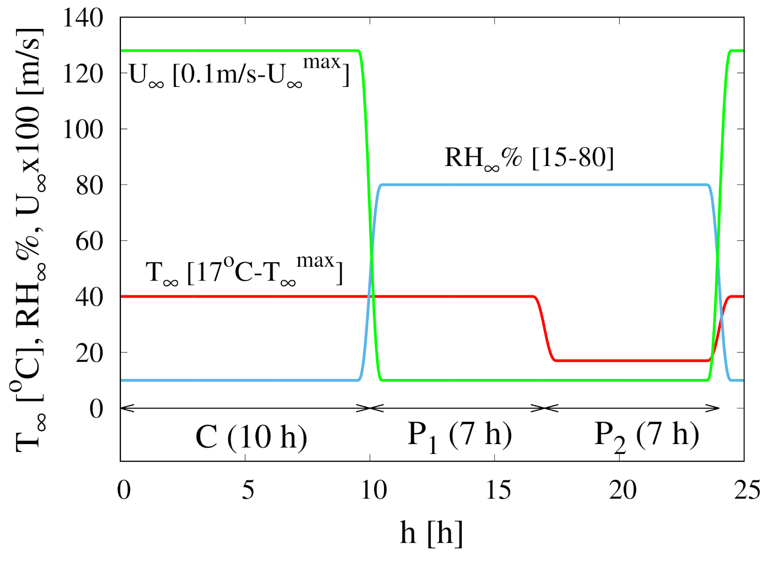
- 1.
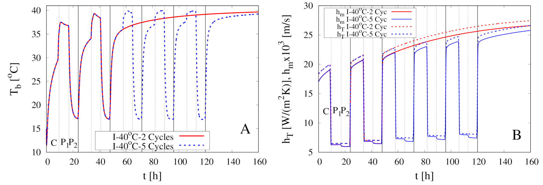
- A first stage (10 h) of convective drying (C) with air velocity or m/s, high temperature C or 50 C and low Relative Humidity .
- 2.
- A second pause stage (, 7 h), simulating the barreling stage, characterized by a high temperature C, 50 C, high Relative Humidity and very low air velocity m/s.
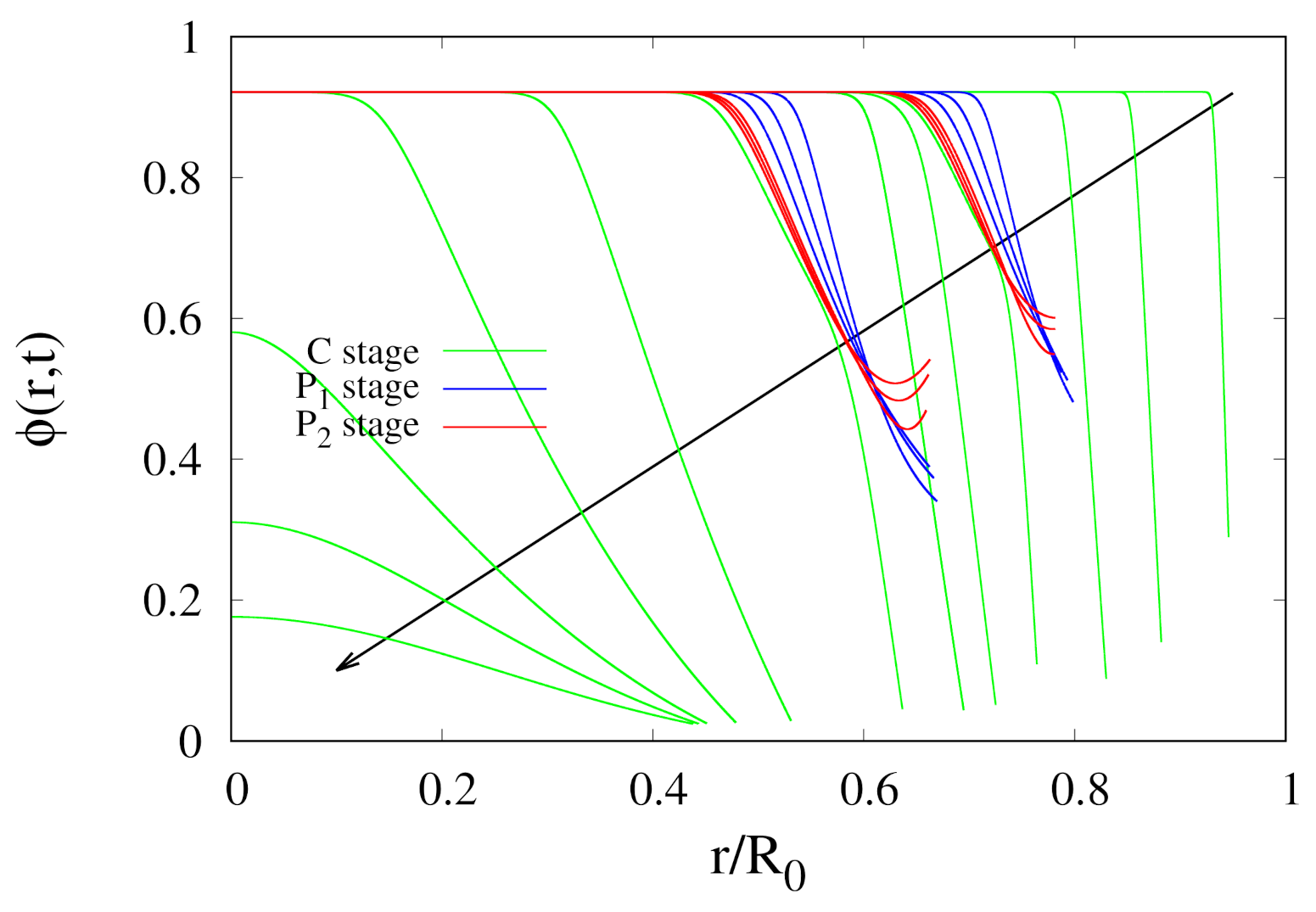
- 3.
- A third pause stage (, 7 h), simulating the night period, characterized by a low temperature C, high Relative Humidity and very low air velocity m/s.
3. Isothermal and Non-Isothermal Moving-Boundary Models
3.1. Isothermal Moving-Boundary Model
3.2. Non-Isothermal Moving-Boundary Model
3.3. Numerical Issues
4. Modeling of Continuous Drying Experiments
4.1. The Isothermal Approach
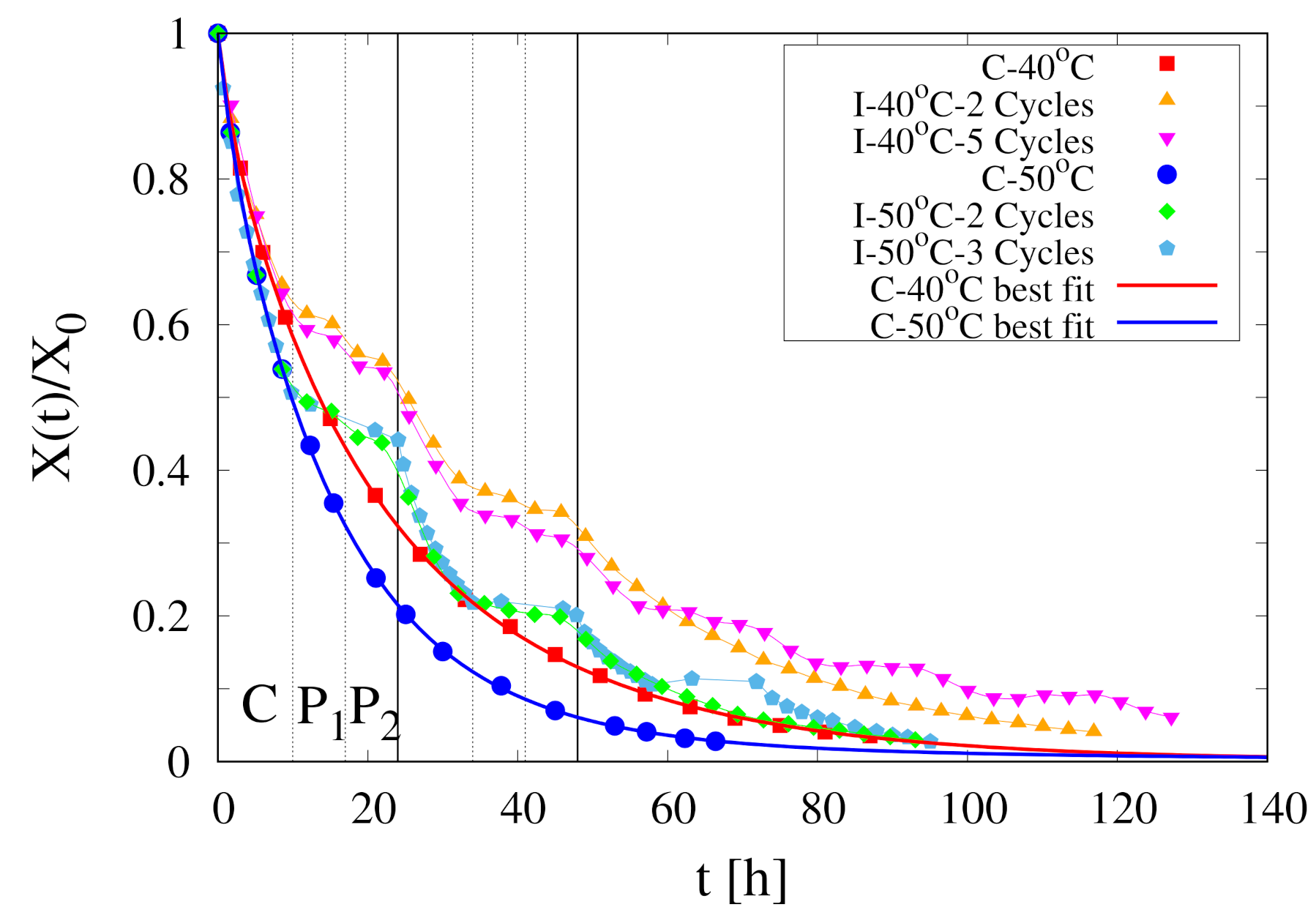
- 1.
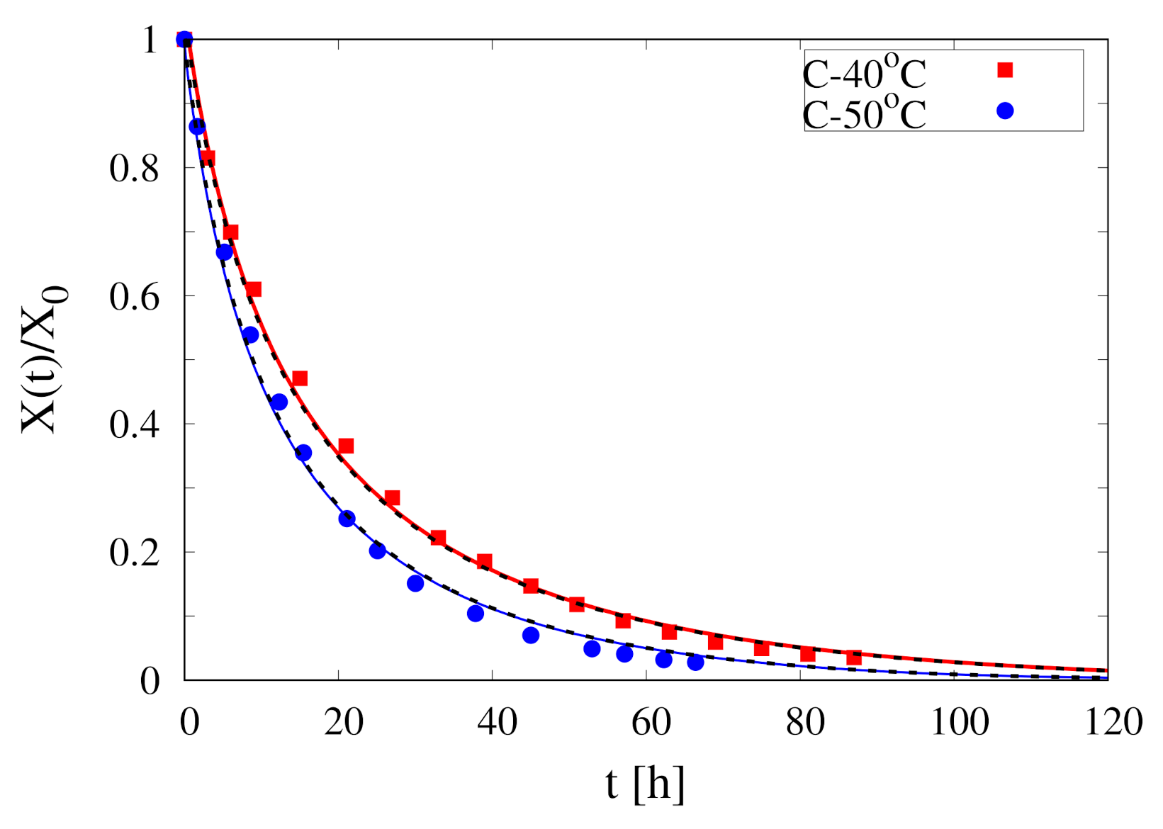
- By direct comparison between experimental continuous dehydration curves at C and C (see Figure 2) it can be observed that is highly sensitive to air temperature
- 2.
- The initial temperature of the sample in all the experiments is C, well below the operating temperature C, 50 C
- 3.
- The initial moisture content of Rocha pears is high, order of 5–6 kg water/kg dry solid, that implies an initial water weight fraction . To make a rough calculation, at the beginning of the drying process, the product density , the specific heat capacity and the thermal conductivity can be reasonably approximated with that of water.A sphere of non evaporating water with diameter cm requires about five hours to rise its temperature from 15 C to 40 C for a heat transfer coefficient W/(m K).
- 4.
- Given the high dehydration rates, especially at the beginning of the drying process, most part of the heat flux supplied by forced convection is used for water evaporation at the air/sample interface. Therefore, the time required to rise the sample temperature from 15 C to 40 C could reasonably increase from 5 to more than 30 h.
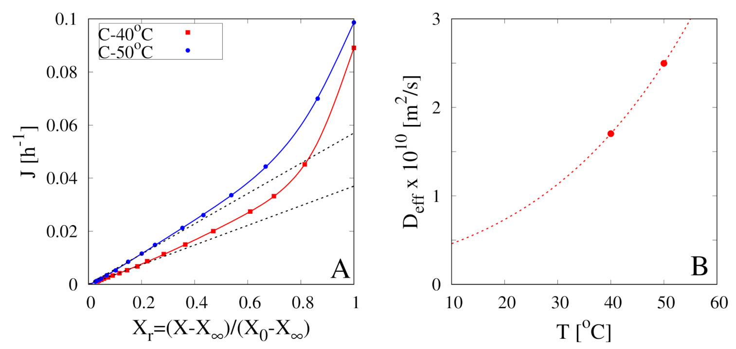
4.2. The Estimate of from the Asymptotic Behavior of Dehydration-Rate Curves
4.3. The Non-Isothermal Approach
5. Modeling of Intermittent Drying Experiments
6. Conclusions
Author Contributions
Funding
Conflicts of Interest
Nomenclature
| Symbols | ||
| [-] | Water activity | |
| [-] | Asymptotic Biot number, Equation (A16) | |
| [g water/m product] | Water mass concentration | |
| ,, | [J/(g K)] | Product, solid and water specific heat capacity |
| ,, | [W/(m K)] | Product, solid and water thermal conductivity |
| d | [m] | Sample diameter |
| [m/s] | Effective water diffusivity | |
| [m/s] | Vapor in air diffusivity | |
| [m/s] | Air thermal diffusivity | |
| [m/s] | Product thermal diffusivity | |
| [m/s] | Mass transfer coefficient | |
| [W/(m K)] | Heat transfer coefficient | |
| J | [h] | Dehydration rate |
| [g water/(s m)] | Water diffusive mass flux | |
| [W/(m K)] | Air thermal conductivity | |
| [-] | Equilibrium constant, Equation (A3) | |
| [-] | Nusselt number | |
| p | [Pa] | Vapor partial pressure |
| [Pa] | Saturated vapor pressure | |
| [-] | Prandl number | |
| r | [m] | Radial coordinate |
| R | [m] | Sample radius |
| [J/(mol K)] | Gas constant | |
| [-] | Reynolds number | |
| [-] | Relative humidity | |
| [-] | Schmidt number | |
| [-] | Sherwood | |
| t | [s] | Time |
| T | [K] | Temperature |
| [K] | Average film temperature | |
| V | [m] | Sample volume |
| [m/s] | Shrinkage velocity | |
| [-] | Water weight fraction | |
| X | [kg water/kg dry solid] | Total moisture content |
| Greek Symbols | ||
| [-] | Shrinkage factor | |
| [-] | smallest positive root of Equation (A18) | |
| [J/g] | Heat of water vaporization | |
| [m/s] | Air kinematic viscosity | |
| [g product/cm product] | Product density | |
| [g solid/cm solid] | Solid (pulp) density | |
| [g water/cm water] | Water density | |
| [-] | water volume fraction | |
| Subscripts | ||
| 0 | Initial | |
| b | Sample surface (boundary) | |
| Equilibrium | ||
| ∞ | Asymptotic or at infinite distance |
Appendix A

Appendix B
- 1.
- the sample temperature has already reached its asymptotic value
- 2.
- the sample radius can be approximated with its asymptotic value
- 3.
- the convective-shrinkage contribution is negligible compared to the diffusive term , and a purely diffusive transport equation can be adopted
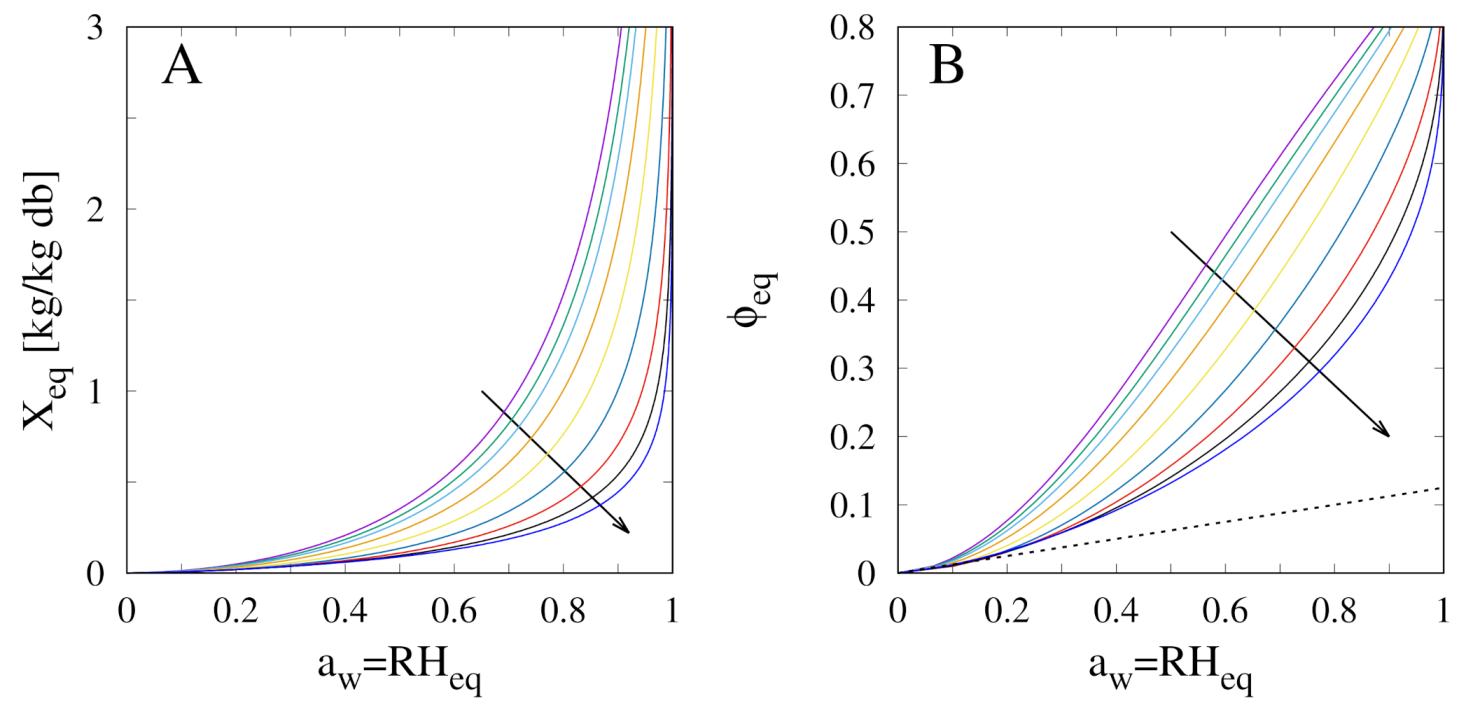
- 4.
- the nonlinear desorption isotherm at can be approximated with a linear behaviour valid for small , Equation (A3), shown in Figure A1B (black dashed line). Therefore, Equation (A14) can be solved with the simplified boundary conditionswhere , and represents the asymptotic mass Biot number
References
- Sagar, V.; Suresh Kumar, P. Recent advances in drying and dehydration of fruits and vegetables: A review. J. Food Sci. Technol. 2010, 47, 15–26. [Google Scholar] [CrossRef] [PubMed]
- Mayor, L.; Sereno, A. Modelling shrinkage during convective drying of food materials: A review. J. Food Eng. 2004, 61, 373–386. [Google Scholar] [CrossRef]
- Mahiuddin, M.; Khan, M.; Kumar, C.; Rahman, M.; Karim, M. Shrinkage of Food Materials During Drying: Current Status and Challenges. Compr. Rev. Food Sci. Food Saf. 2018, 17, 1113–1126. [Google Scholar] [CrossRef]
- Castro, A.; Mayorga, E.; Moreno, F. Mathematical modelling of convective drying of fruits: A review. J. Food Eng. 2018, 223, 152–167. [Google Scholar] [CrossRef]
- Baini, R.; Langrish, T. Choosing an appropriate drying model for intermittent and continuous drying of bananas. J. Food Eng. 2007, 79, 330–343. [Google Scholar] [CrossRef]
- Kowalski, S.; Pawłowski, A. Energy consumption and quality aspect by intermittent drying. Chem. Eng. Process. Process Intensif. 2011, 50, 384–390. [Google Scholar] [CrossRef]
- Kowalski, S.J.; Szadzińska, J.; Łechtańska, J. Non-stationary drying of carrot: Effect on product quality. J. Food Eng. 2013, 118, 393–399. [Google Scholar] [CrossRef]
- Yang, Z.; Zhu, E.; Zhu, Z.; Wang, J.; Li, S. A comparative study on intermittent heat pump drying process of Chinese cabbage (Brassica campestris L. ssp) seeds. Food Bioprod. Process. 2013, 91, 381–388. [Google Scholar] [CrossRef]
- Silva, V.; Figueiredo, A.; Costa, J.; Guiné, R. Experimental and mathematical study of the discontinuous drying kinetics of pears. J. Food Eng. 2014, 134, 30–36. [Google Scholar] [CrossRef]
- da Silva, W.P.; Rodrigues, A.F.; e Silva, C.M.D.; de Castro, D.S.; Gomes, J.P. Comparison between continuous and intermittent drying of whole bananas using empirical and diffusion models to describe the processes. J. Food Eng. 2015, 166, 230–236. [Google Scholar] [CrossRef]
- Silva, V.; Costa, J.J.; Figueiredo, A.R.; Nunes, J.; Nunes, C.; Ribeiro, T.I.; Pereira, B. Study of three-stage intermittent drying of pears considering shrinkage and variable diffusion coefficient. J. Food Eng. 2016, 180, 77–86. [Google Scholar] [CrossRef]
- Lozano, J.E.; Rotstein, E.; Urbicain, M.J. Shrinkage, Porosity and Bulk Density of Foodstuffs at Changing Moisture Contents. J. Food Sci. 1983, 48, 1497–1502. [Google Scholar] [CrossRef]
- Adrover, A.; Brasiello, A.; Ponso, G. A moving boundary model for food isothermal drying and shrinkage: General setting. J. Food Eng. 2019, 244, 178–191. [Google Scholar] [CrossRef]
- Adrover, A.; Brasiello, A.; Ponso, G. A moving boundary model for food isothermal drying and shrinkage: A shortcut numerical method for estimating the shrinkage factor. J. Food Eng. 2019, 244, 212–219. [Google Scholar] [CrossRef]
- Adrover, A.; Brasiello, A. A Moving Boundary Model for Isothermal Drying and Shrinkage of Chayote Discoid Samples: Comparison between the Fully Analytical and the Shortcut Numerical Approaches. Int. J. Chem. Eng. 2019, 2019, 3926897. [Google Scholar] [CrossRef]
- Adrover, A.; Brasiello, A. A moving boundary model for food isothermal drying and shrinkage: One-dimensional versus two-dimensional approaches. J. Food Process. Eng. 2019, 42, e13178. [Google Scholar] [CrossRef]
- Adrover, A.; Brasiello, A. 3-D Modeling of Dehydration Kinetics and Shrinkage of Ellipsoidal Fermented Amazonian Cocoa Beans. Processes 2020, 8, 150. [Google Scholar] [CrossRef]
- Papanu, J.; Soane (Soong), D.; Bell, A.; Hess, D. Transport models for swelling and dissolution of thin polymer films. J. Appl. Polym. Sci. 1989, 38, 859–885. [Google Scholar] [CrossRef]
- Tu, Y.O.; Ouano, A.C. Model for the kinematics of polymer dissolution. IBM J. Res. Dev. 1977, 21, 131–142. [Google Scholar] [CrossRef]
- Crank, J. Free and Moving Boundary Problems; Clarendon Press: Oxford, UK, 1987. [Google Scholar]
- Adrover, A.; Nobili, M. Release kinetics from oral thin films: Theory and experiments. Chem. Eng. Res. Des. 2015, 98, 188–201. [Google Scholar] [CrossRef]
- Carslaw, H.; Jaeger, J. Conduction of Heat in Solids, 2nd ed.; Oxford University Press: Oxford, UK, 1959. [Google Scholar]
- Hahn, D.W.; Ozisik, M.N. Heat Conduction, 3rd ed.; Wiley: Hoboken, NJ, USA, 2012. [Google Scholar]
- Herman, C.; Spreutels, L.; Turomzsa, N.; Konagano, E.M.; Haut, B. Convective drying of fermented Amazonian cocoa beans (Theobroma cacao var. Forasteiro). Experiments and mathematical modeling. Food Bioprod. Process. 2018, 108, 81–94. [Google Scholar] [CrossRef]
- Hii, C.; Law, C.; Law, M. Simulation of heat and mass transfer of cocoa beans under stepwise drying conditions in a heat pump dryer. Appl. Therm. Eng. 2013, 54, 264–271. [Google Scholar] [CrossRef]
- Golestani, R.; Raisi, A.; Aroujalian, A. Mathematical Modeling on Air Drying of Apples Considering Shrinkage and Variable Diffusion Coefficient. Dry. Technol. 2013, 31, 40–51. [Google Scholar] [CrossRef]
- Guiné, R.P.F. Sorption Isotherms of Pears Using Different Models. Int. J. Fruit Sci. 2009, 9, 11–22. [Google Scholar] [CrossRef]
- Srikiatden, J.; Roberts, J.S. Measuring moisture diffusivity of potato and carrot (core and cortex) during convective hot air and isothermal drying. J. Food Eng. 2006, 74, 143–152. [Google Scholar] [CrossRef]
- Srikiatden, J.; Roberts, J.S. Predicting moisture profiles in potato and carrot during convective hot air drying using isothermally measured effective diffusivity. J. Food Eng. 2008, 84, 516–525. [Google Scholar] [CrossRef]
- Dong, R.; Lu, Z.; Liu, Z.; Koide, S.; Cao, W. Effect of drying and tempering on rice fissuring analysed by integrating intra-kernel moisture distribution. J. Food Eng. 2010, 97, 161–167. [Google Scholar] [CrossRef]
- Guiné, R.P.F.; Castro, J.A.A.M. Analysis of Moisture Content and Density of Pears During Drying. Dry. Technol. 2003, 21, 581–591. [Google Scholar] [CrossRef]
- Rahman, M.; Chen, X.; Perera, C. An improved thermal conductivity prediction model for fruits and vegetables as a function of temperature, water content and porosity. J. Food Eng. 1997, 31, 163–170. [Google Scholar] [CrossRef]
- Becker, B.; Fricke, B. FREEZING | Principles. In Encyclopedia of Food Sciences and Nutrition, 2nd ed.; Caballero, B., Ed.; Academic Press: Oxford, UK, 2003; pp. 2706–2711. [Google Scholar] [CrossRef]
- Bird, R.B.; Stewart, W.E.; Lightfoot, E.N. Transport Phenomena, 2nd ed.; Wiley: Hoboken, NJ, USA, 2006. [Google Scholar]
- Tsilingiris, P. Thermophysical and transport properties of humid air at temperature range between 0 and 100 °C. Energy Convers. Manag. 2008, 49, 1098–1110. [Google Scholar] [CrossRef]
- Boukhriss, M.; Zhani, K.; Ghribi, R. Study of thermophysical properties of a solar desalination system using solar energy. Desalin. Water Treat. 2013, 51, 1290–1295. [Google Scholar] [CrossRef]
- Still, M.; Venzke, H.; Durst, F.; Melling, A. Influence of humidity on the convective heat transfer from small cylinders. Exp. Fluids 1998, 24, 141–150. [Google Scholar] [CrossRef]
- Crank, J. The Mathematics of Diffusion; Clarendon Press: Oxford, UK, 1979. [Google Scholar]


| Experiment | Type | Cycles | ||||
|---|---|---|---|---|---|---|
| [C] | [m/s] | [cm] | ||||
| C-40 C * | C | - | 40 | 1.28 | 5.64 | 5.30 |
| I-40 C-2 Cycles * | I | 2 | 40 | 1.28 | 6.48 | 5.36 |
| I-40 C-5 Cycles * | I | 5 | 40 | 1.28 | 5.37 | 5.30 |
| C-50 C * | C | - | 50 | 1.28 | 5.55 | 5.24 |
| I-50 C-2 Cycles * | I | 2 | 50 | 1.28 | 6.21 | 5.32 |
| I-50 C-3 Cycles I * | I | 3 | 50 | 1.28 | 6.25 | 5.69 |
| I-50 C-3 Cycles II ** | I | 3 | 50 | 2.66 | 7.24 | 5.43 |
Publisher’s Note: MDPI stays neutral with regard to jurisdictional claims in published maps and institutional affiliations. |
© 2020 by the authors. Licensee MDPI, Basel, Switzerland. This article is an open access article distributed under the terms and conditions of the Creative Commons Attribution (CC BY) license (http://creativecommons.org/licenses/by/4.0/).
Share and Cite
Adrover, A.; Venditti, C.; Brasiello, A. A Non-Isothermal Moving-Boundary Model for Continuous and Intermittent Drying of Pears. Foods 2020, 9, 1577. https://doi.org/10.3390/foods9111577
Adrover A, Venditti C, Brasiello A. A Non-Isothermal Moving-Boundary Model for Continuous and Intermittent Drying of Pears. Foods. 2020; 9(11):1577. https://doi.org/10.3390/foods9111577
Chicago/Turabian StyleAdrover, Alessandra, Claudia Venditti, and Antonio Brasiello. 2020. "A Non-Isothermal Moving-Boundary Model for Continuous and Intermittent Drying of Pears" Foods 9, no. 11: 1577. https://doi.org/10.3390/foods9111577
APA StyleAdrover, A., Venditti, C., & Brasiello, A. (2020). A Non-Isothermal Moving-Boundary Model for Continuous and Intermittent Drying of Pears. Foods, 9(11), 1577. https://doi.org/10.3390/foods9111577