
Predicting the Moisture Ratio of a Hami Melon Drying Process Using Image Processing Technology


Abstract
:1. Introduction
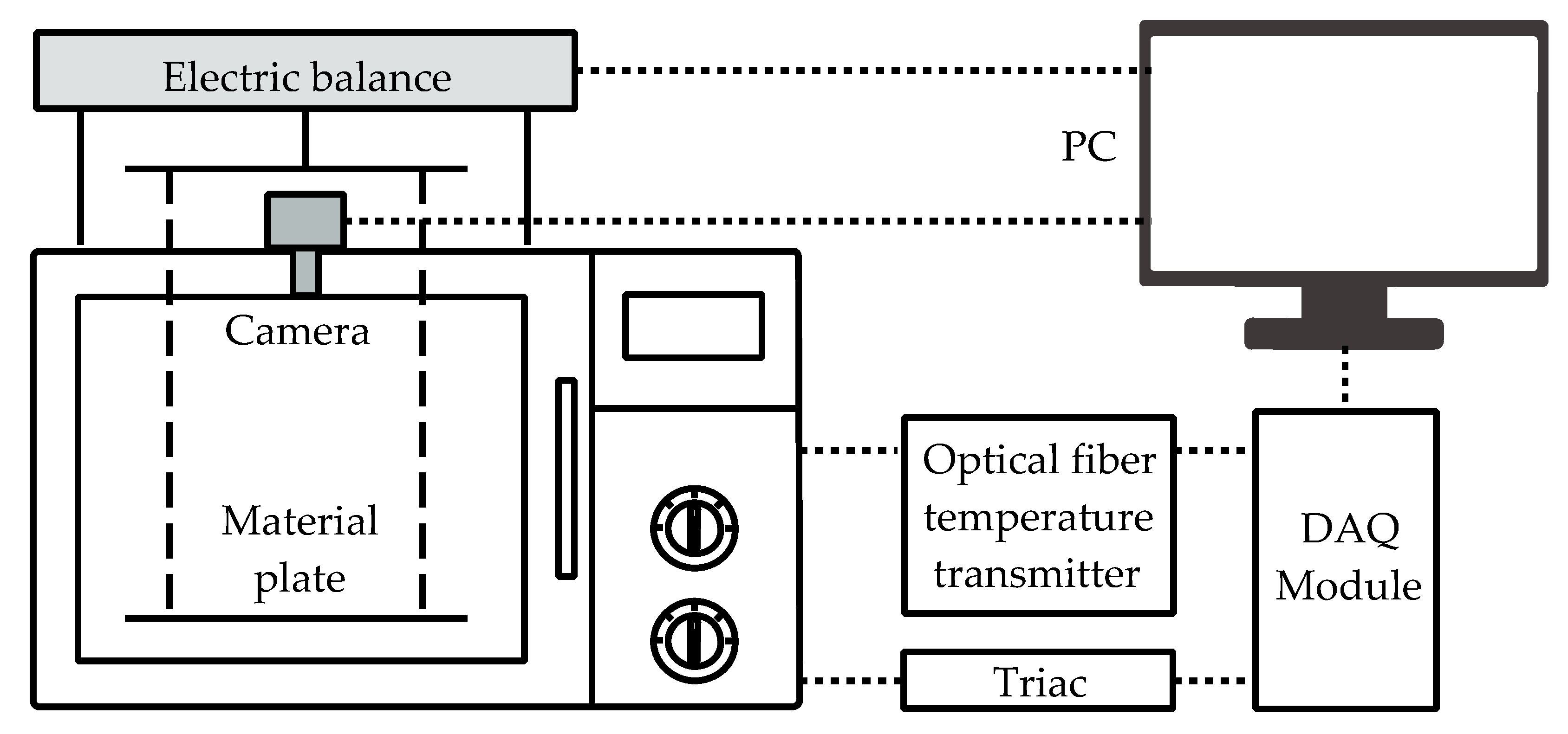
- An experimental system that included an adjustable-power microwave drying unit and an image-processing unit was developed, and the moisture content and the area of samples at different times during the Hami melon drying process were collected.
- The representation of the moisture ratio with regard to the shrinkage of the drying process of Hami melon slices was assumed by means of the Weierstrass approximation theorem.
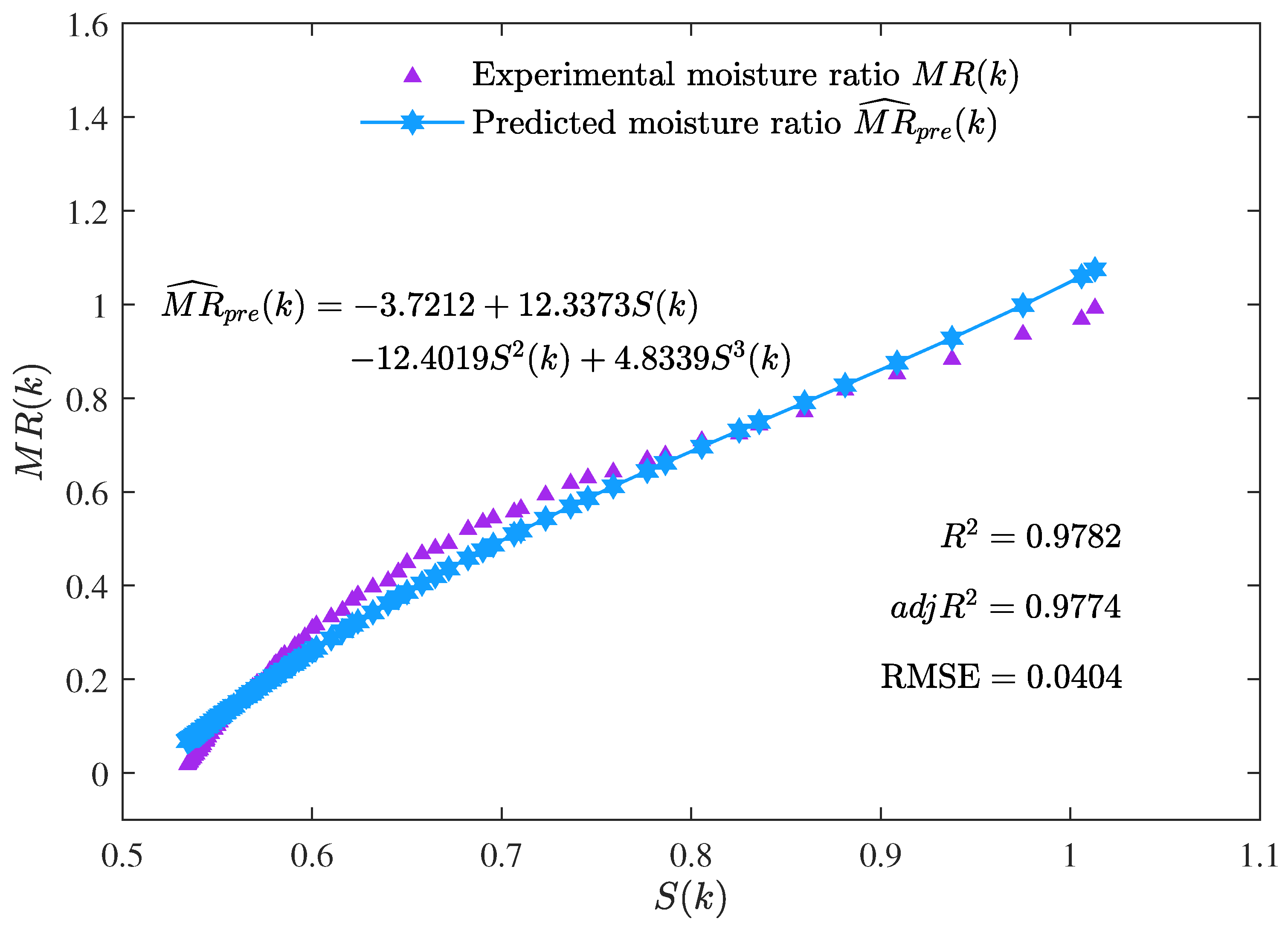
- By deducing the maximum likelihood fitness function, a maximum likelihood fitness function-based population evolution (MLFF-PE) algorithm was presented to fit the moisture ratio model and predict the moisture ratio changes in the drying process of Hami melon slices. The results showed that the estimated moisture ratio model given by the MLFF-PE algorithm performed well in the moisture ratio model’s fitting and the moisture ratio prediction of the Hami melon drying process.
2. Materials and Methods
2.1. Materials
2.2. Microwave Drying System Based on Image Processing
2.3. Experimental Details
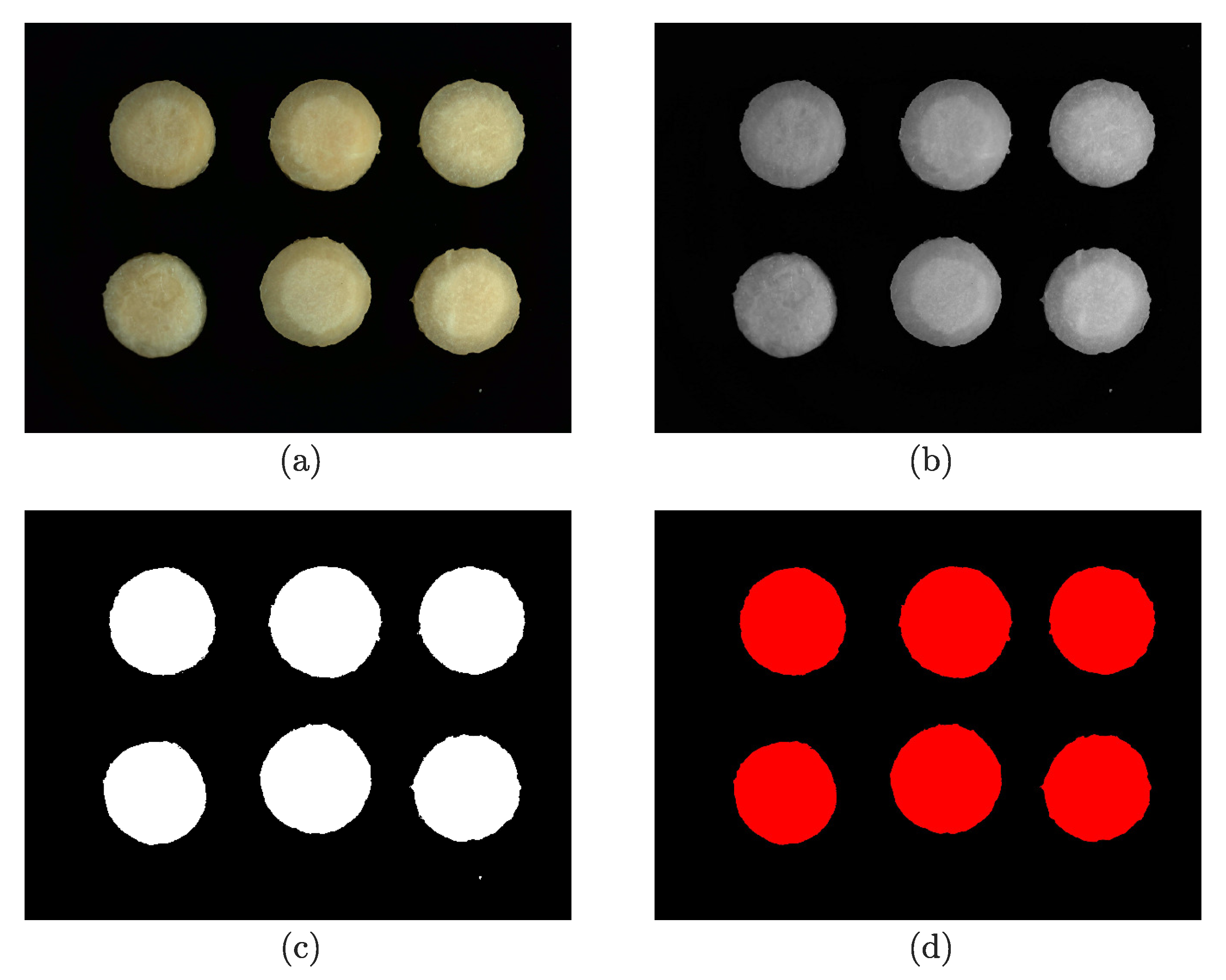
2.4. Image Processing Algorithm
3. Mathematical Model
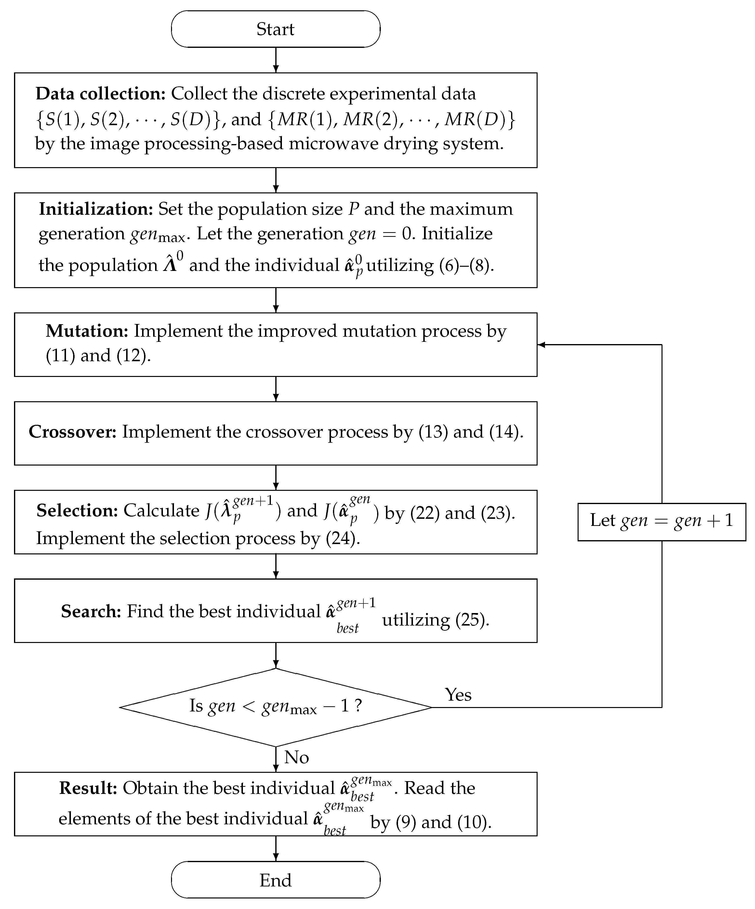
4. MLFF-PE Method
4.1. Population Initialization
4.2. Mutation Process
4.3. Crossover Process
4.4. Maximum Likelihood Fitness Function
4.5. Selection Process
5. Modeling and Prediction
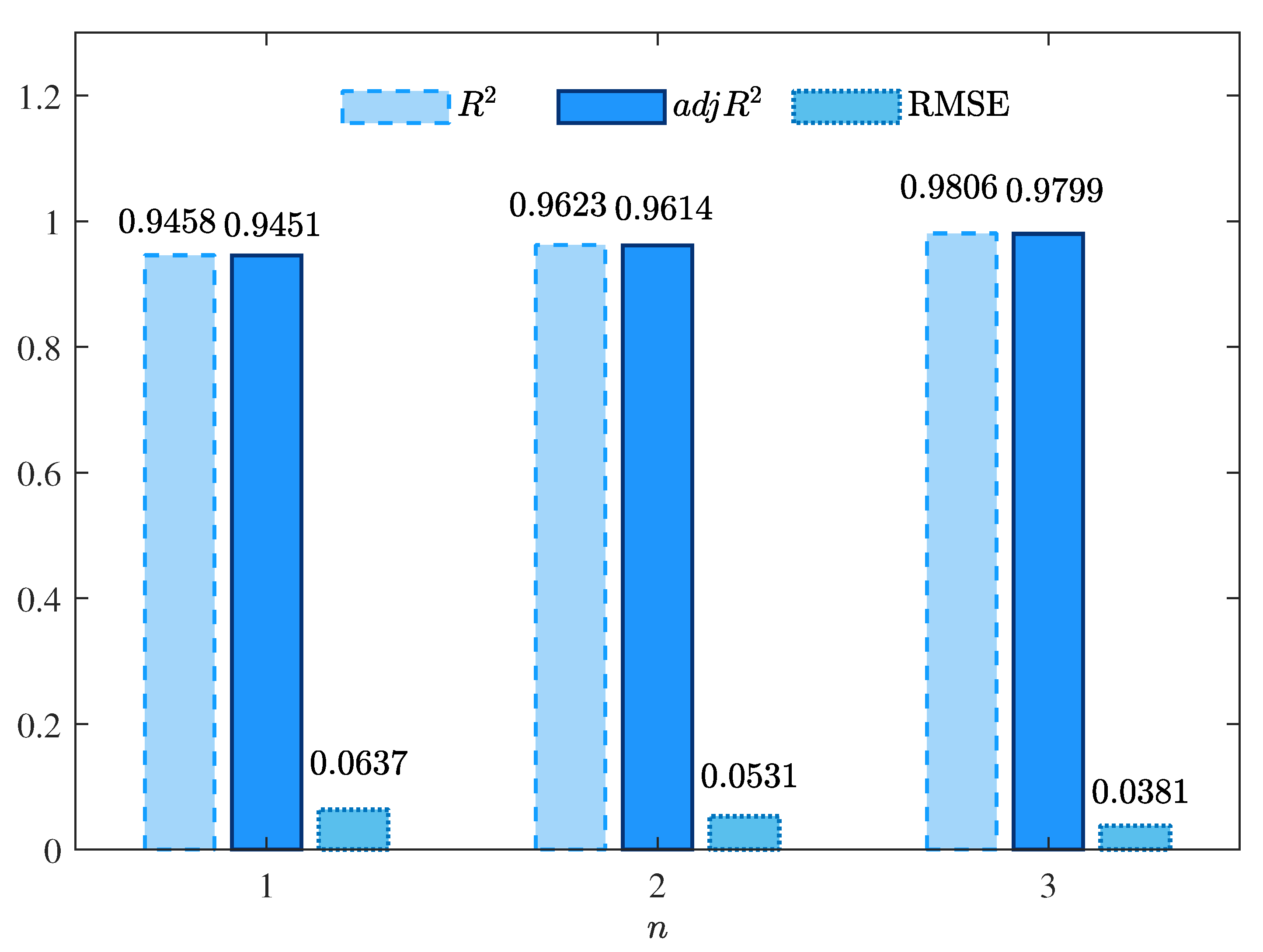
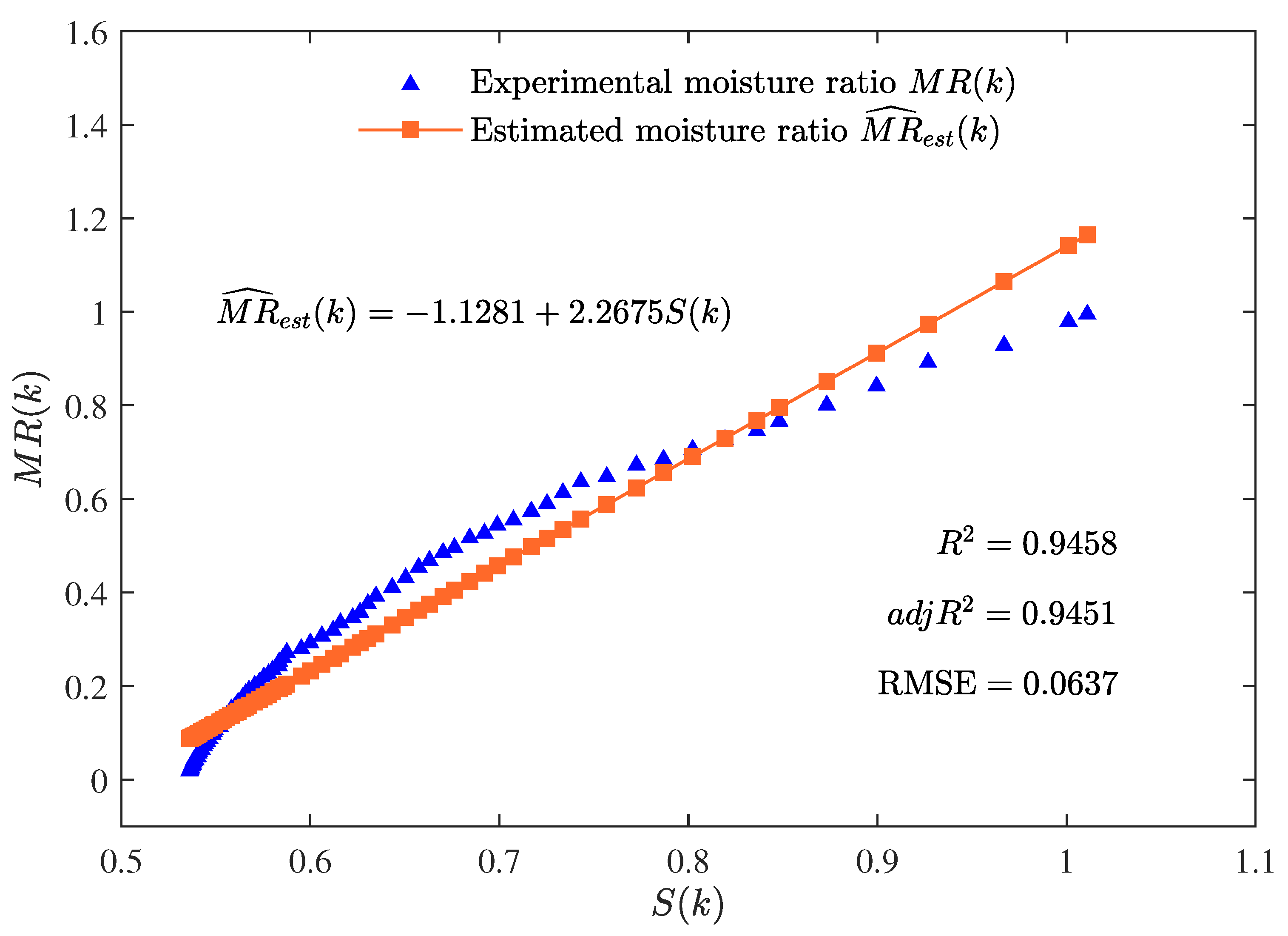
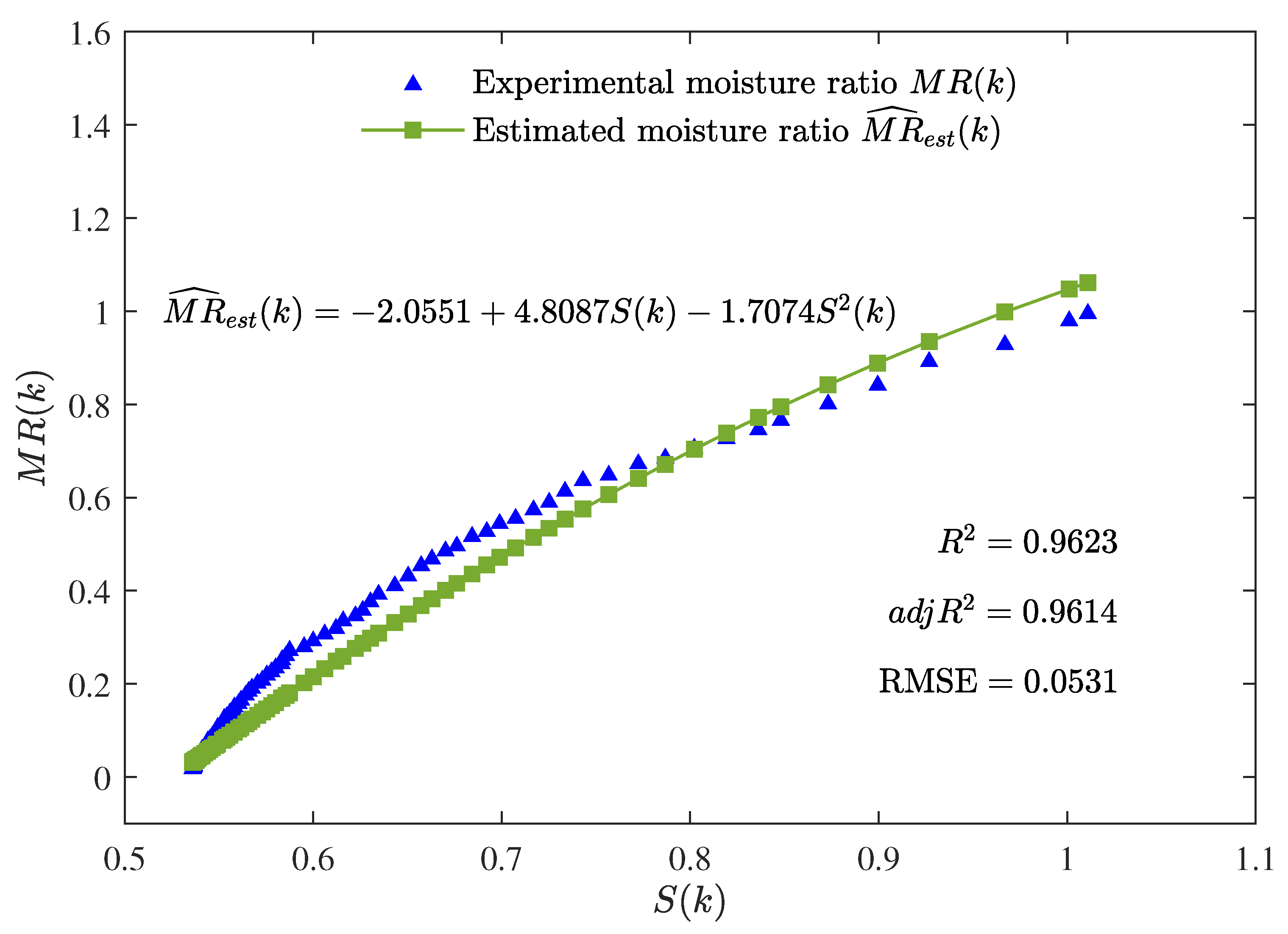
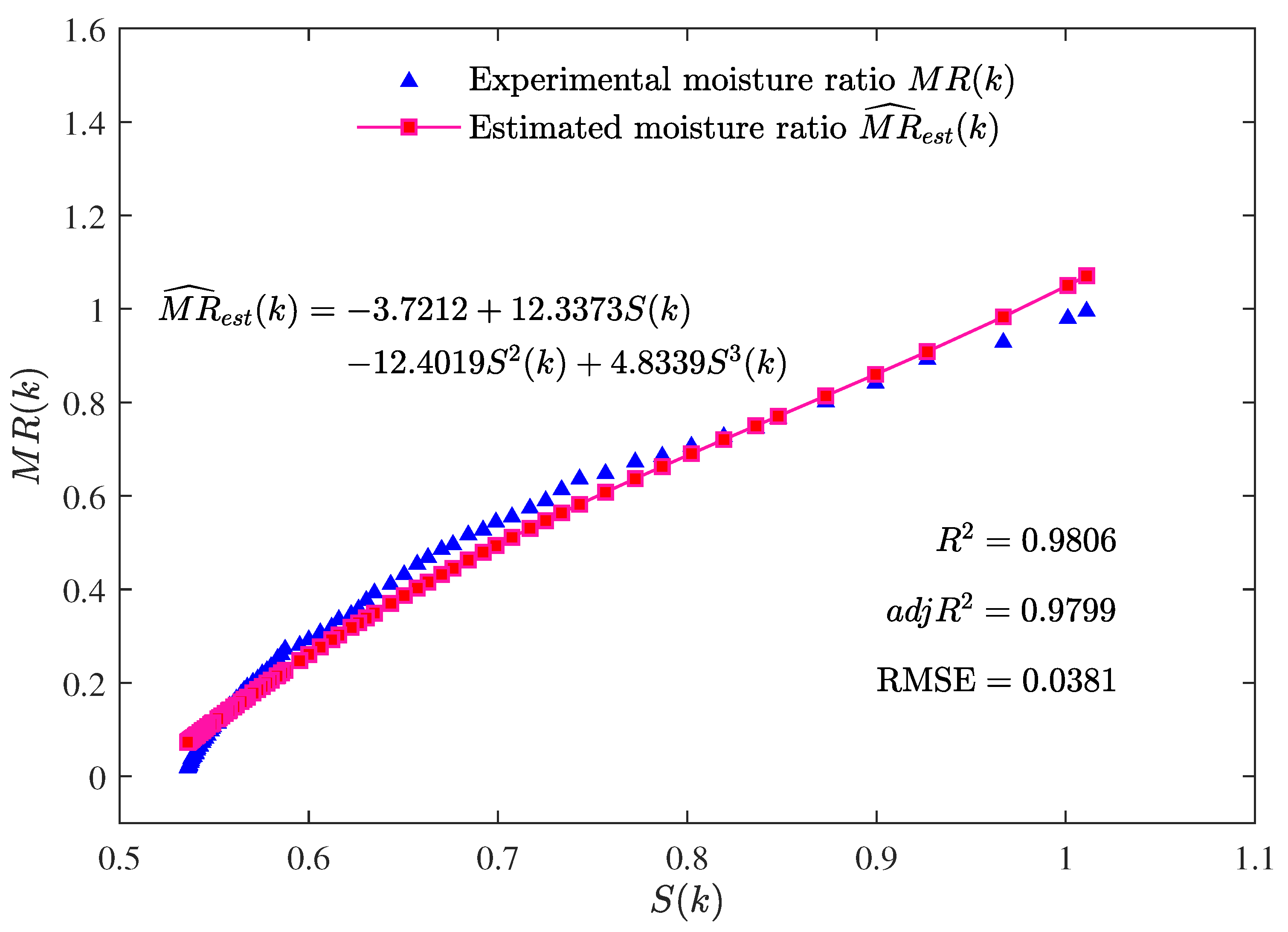
5.1. Model Fitting
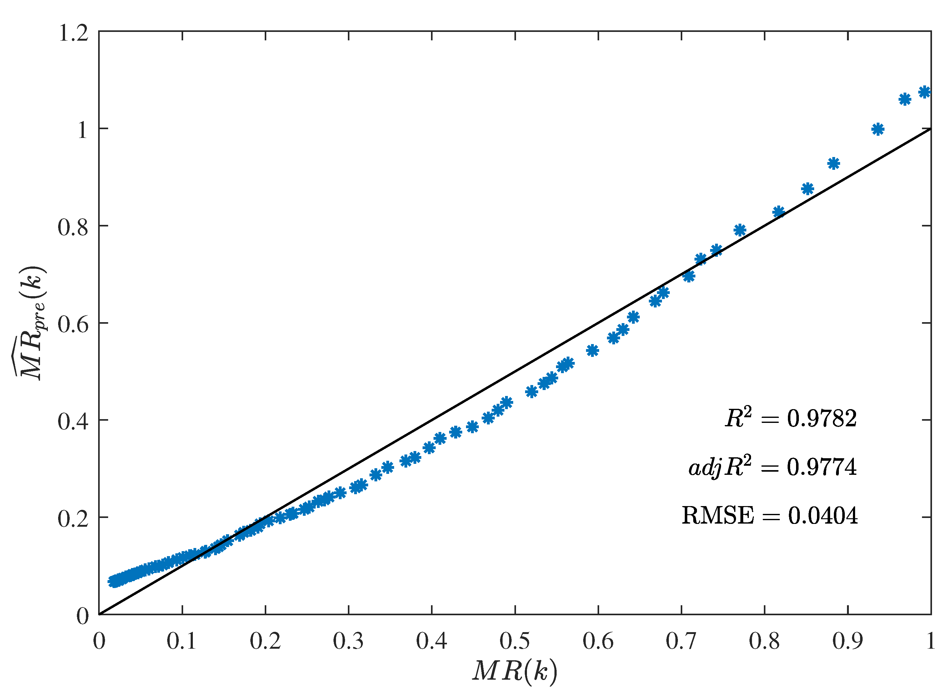
5.2. Prediction
5.3. Results and Discussion
6. Conclusions
Author Contributions
Funding
Institutional Review Board Statement
Informed Consent Statement
Data Availability Statement
Conflicts of Interest
References
- Pinho, L.S.; de Lima, P.M.; de Sá, S.H.G.; Chen, D.; Campanella, O.H.; da Costa Rodrigues, C.E.; Favaro-Trindade, C.S. Encapsulation of Rich-Carotenoids Extract from Guaraná (Paullinia cupana) Byproduct by a Combination of Spray Drying and Spray Chilling. Foods 2022, 11, 2557. [Google Scholar] [CrossRef]
- Jiang, C.; Wan, F.; Zang, Z.; Zhang, Q.; Ma, G.; Huang, X. Effect of an Ultrasound Pre-Treatment on the Characteristics and Quality of Far-Infrared Vacuum Drying with Cistanche Slices. Foods 2022, 11, 866. [Google Scholar] [CrossRef]
- Li, D.; Chen, R.; Liu, J.; Liu, C.; Deng, L.; Chen, J. Characterizing and alleviating the browning of Choerospondias axillaris fruit cake during drying. Food Control 2022, 132, 108522. [Google Scholar] [CrossRef]
- Arefi, A.; Sturm, B.; von Gersdorff, G.; Nasirahmadi, A.; Hensel, O. Vis-NIR hyperspectral imaging along with Gaussian process regression to monitor quality attributes of apple slices during drying. LWT 2021, 152, 112297. [Google Scholar] [CrossRef]
- Macedo, L.L.; Corrêa, J.L.G.; da Silva Araújo, C.; Vimercati, W.C.; Júnior, I.P. Convective drying with ethanol pre-treatment of strawberry enriched with isomaltulose. Food Bioprocess Technol. 2021, 14, 2046–2061. [Google Scholar] [CrossRef]
- César, L.V.E.; Lilia, C.M.A.; Octavio, G.V.; Isaac, P.F.; Rogelio, B.O. Thermal performance of a passive, mixed-type solar dryer for tomato slices (Solanum lycopersicum). Renew. Energy 2020, 147, 845–855. [Google Scholar] [CrossRef]
- Rashidi, M.; Chayjan, R.A.; Ghasemi, A.; Ershadi, A. Tomato tablet drying enhancement by intervention of infrared-A response surface strategy for experimental design and optimization. Biosyst. Eng. 2021, 208, 199–212. [Google Scholar] [CrossRef]
- Michalska-Ciechanowska, A.; Hendrysiak, A.; Brzezowska, J.; Wojdyło, A.; Gajewicz-Skretna, A. How Do the Different Types of Carrier and Drying Techniques Affect the Changes in Physico-Chemical Properties of Powders from Chokeberry Pomace Extracts? Foods 2021, 10, 1864. [Google Scholar] [CrossRef]
- Raghavan, G.; Silveira, A. Shrinkage characteristics of strawberries osmotically dehydrated in combination with microwave drying. Dry. Technol. 2001, 19, 405–414. [Google Scholar] [CrossRef]
- Chen, X.; Liu, Y.; Zhang, R.; Zhu, H.; Li, F.; Yang, D.; Jiao, Y. Radio Frequency Drying Behavior in Porous Media: A Case Study of Potato Cube with Computer Modeling. Foods 2022, 11, 3279. [Google Scholar] [CrossRef]
- Paul, A.; Martynenko, A. The Effect of Material Thickness, Load Density, External Airflow, and Relative Humidity on the Drying Efficiency and Quality of EHD-Dried Apples. Foods 2022, 11, 2765. [Google Scholar] [CrossRef] [PubMed]
- Lazzarini, C.; Casadei, E.; Valli, E.; Tura, M.; Ragni, L.; Bendini, A.; Gallina Toschi, T. Sustainable Drying and Green Deep Eutectic Extraction of Carotenoids from Tomato Pomace. Foods 2022, 11, 405. [Google Scholar] [CrossRef]
- Geng, Z.; Huang, X.; Wang, J.; Xiao, H.; Yang, X.; Zhu, L.; Qi, X.; Zhang, Q.; Hu, B. Pulsed vacuum drying of pepper (Capsicum annuum L.): Effect of high-humidity hot air impingement blanching pretreatment on drying kinetics and quality attributes. Foods 2022, 11, 318. [Google Scholar] [CrossRef]
- Giri, S.; Prasad, S. Modeling shrinkage and density changes during microwave-vacuum drying of button mushroom. Int. J. Food Prop. 2006, 9, 409–419. [Google Scholar] [CrossRef]
- Hernandez, J.; Pavon, G.; Garcıa, M. Analytical solution of mass transfer equation considering shrinkage for modeling food-drying kinetics. J. Food Eng. 2000, 45, 1–10. [Google Scholar] [CrossRef]
- Frias, A.; Clemente, G.; Mulet, A. Potato shrinkage during hot air drying. Food Sci. Technol. Int. 2010, 16, 337–341. [Google Scholar] [CrossRef] [PubMed]
- Yadollahinia, A.; Latifi, A.; Mahdavi, R. New method for determination of potato slice shrinkage during drying. Comput. Electron. Agric. 2009, 65, 268–274. [Google Scholar] [CrossRef]
- Afonso, P.; Correa, P.; Pinto, F.; Sampaio, C. Shrinkage evaluation of five different varieties of coffee berries during the drying process. Biosyst. Eng. 2003, 86, 481–485. [Google Scholar] [CrossRef]
- Ramallo, L.A.; Mascheroni, R.H. Effect of shrinkage on prediction accuracy of the water diffusion model for pineapple drying. J. Food Process Eng. 2013, 36, 66–76. [Google Scholar] [CrossRef]
- Raponi, F.; Moscetti, R.; Chakravartula, S.S.N.; Fidaleo, M.; Massantini, R. Monitoring the hot-air drying process of organically grown apples (cv. Gala) using computer vision. Biosyst. Eng. 2022, 223, 1–13. [Google Scholar] [CrossRef]
- Lin, X.; Sun, D.W. Development of a general model for monitoring moisture distribution of four vegetables undergoing microwave-vacuum drying by hyperspectral imaging. Dry. Technol. 2021, 40, 1478–1492. [Google Scholar] [CrossRef]
- Jiménez-Carvelo, A.M.; Cruz, C.M.; Cuadros-Rodríguez, L.; Koidis, A. Machine learning techniques in food processing. In Current Developments in Biotechnology and Bioengineering; Elsevier: Amsterdam, The Netherlands, 2022; pp. 333–351. [Google Scholar]
- Salehi, F. Recent advances in the modeling and predicting quality parameters of fruits and vegetables during postharvest storage: A review. Int. J. Fruit Sci. 2020, 20, 506–520. [Google Scholar] [CrossRef]
- Kucheryavski, S.; Esbensen, K.H.; Bogomolov, A. Monitoring of pellet coating process with image analysis—a feasibility study. J. Chemom. 2010, 24, 472–480. [Google Scholar] [CrossRef]
- Madiouli, J.; Sghaier, J.; Orteu, J.J.; Robert, L.; Lecomte, D.; Sammouda, H. Non-contact measurement of the shrinkage and calculation of porosity during the drying of banana. Dry. Technol. 2011, 29, 1358–1364. [Google Scholar] [CrossRef]
- Huang, M.; Wang, Q.; Zhang, M.; Zhu, Q. Prediction of color and moisture content for vegetable soybean during drying using hyperspectral imaging technology. J. Food Eng. 2014, 128, 24–30. [Google Scholar] [CrossRef]
- Nahimana, H.; Zhang, M. Shrinkage and color change during microwave vacuum drying of carrot. Dry. Technol. 2011, 29, 836–847. [Google Scholar] [CrossRef]
- Bonnet, A.; Herrera, M.M.; Sangnier, M. Maximum Likelihood Estimation for Hawkes Processes with self-excitation or inhibition. Stat. Probab. Lett. 2021, 179, 109214. [Google Scholar] [CrossRef]
- Yang, F.; Ren, H.; Hu, Z. Maximum likelihood estimation for three-parameter Weibull distribution using evolutionary strategy. Math. Probl. Eng. 2019, 2019, 6281781. [Google Scholar] [CrossRef]
- Orellana, R.; Bittner, G.; Carvajal, R.; Agüero, J.C. Maximum Likelihood estimation for non-minimum-phase noise transfer function with Gaussian mixture noise distribution. Automatica 2022, 135, 109937. [Google Scholar] [CrossRef]
- Ramadan, M.S.; Bitmead, R.R. Maximum Likelihood recursive state estimation using the Expectation Maximization algorithm. Automatica 2022, 144, 110482. [Google Scholar] [CrossRef]
- Tong, X.; Gao, F.; Chen, K.; Cai, D.; Sun, J. Maximum likelihood estimation in transformed linear regression with nonnormal errors. Ann. Stat. 2019, 47, 1864–1892. [Google Scholar] [CrossRef]
- McGoff, K.; Mukherjee, S.; Nobel, A.; Pillai, N. Consistency of maximum likelihood estimation for some dynamical systems. Ann. Stat. 2015, 43, 1–29. [Google Scholar] [CrossRef]
- Xie, X.; Katselis, D.; Beck, C.L.; Srikant, R. On the Consistency of Maximum Likelihood Estimators for Causal Network Identification. In Proceedings of the 2020 59th IEEE Conference on Decision and Control (CDC), Jeju, Korea, 14–18 December 2020; pp. 990–995. [Google Scholar]
- Wu, M.W.; Jin, Y.; Li, Y.; Song, T.; Kam, P.Y. Maximum-likelihood, magnitude-based, amplitude and noise variance estimation. IEEE Signal Process. Lett. 2021, 28, 414–418. [Google Scholar] [CrossRef]
- Çayır, Ö.; Candan, Ç. Maximum likelihood autoregressive model parameter estimation with noise corrupted independent snapshots. Signal Process. 2021, 186, 108118. [Google Scholar] [CrossRef]
- Xu, W.; Islam, M.N.; Cao, X.; Tian, J.; Zhu, G. Effect of relative humidity on drying characteristics of microwave assisted hot air drying and qualities of dried finger citron slices. Lwt 2021, 137, 110413. [Google Scholar] [CrossRef]
- Luo, G.; Song, C.; Hongjie, P.; Li, Z.; Xu, W.; Raghavan, G.; Chen, H.; Jin, G. Optimization of the microwave drying process for potato chips based on the measurement of dielectric properties. Dry. Technol. 2019, 37, 1329–1339. [Google Scholar] [CrossRef]
- Rezaei, S.; Behroozi-Khazaei, N.; Darvishi, H. Microwave power adjusting during potato slice drying process using machine vision. Comput. Electron. Agric. 2019, 160, 40–50. [Google Scholar] [CrossRef]


| n | RMSE | ||||||
|---|---|---|---|---|---|---|---|
| 1 | −1.1281 | 2.2675 | – | – | 0.9458 | 0.9451 | 0.0637 |
| 2 | −2.0551 | 4.8087 | −1.7074 | – | 0.9623 | 0.9614 | 0.0531 |
| 3 | −3.7212 | 12.3373 | −12.4019 | 4.8339 | 0.9806 | 0.9799 | 0.0381 |
Disclaimer/Publisher’s Note: The statements, opinions and data contained in all publications are solely those of the individual author(s) and contributor(s) and not of MDPI and/or the editor(s). MDPI and/or the editor(s) disclaim responsibility for any injury to people or property resulting from any ideas, methods, instructions or products referred to in the content. |
© 2023 by the authors. Licensee MDPI, Basel, Switzerland. This article is an open access article distributed under the terms and conditions of the Creative Commons Attribution (CC BY) license (https://creativecommons.org/licenses/by/4.0/).
Share and Cite
Zhu, G.; Raghavan, G.S.V.; Li, Z. Predicting the Moisture Ratio of a Hami Melon Drying Process Using Image Processing Technology. Foods 2023, 12, 672. https://doi.org/10.3390/foods12030672
Zhu G, Raghavan GSV, Li Z. Predicting the Moisture Ratio of a Hami Melon Drying Process Using Image Processing Technology. Foods. 2023; 12(3):672. https://doi.org/10.3390/foods12030672
Chicago/Turabian StyleZhu, Guanyu, G.S.V. Raghavan, and Zhenfeng Li. 2023. "Predicting the Moisture Ratio of a Hami Melon Drying Process Using Image Processing Technology" Foods 12, no. 3: 672. https://doi.org/10.3390/foods12030672
APA StyleZhu, G., Raghavan, G. S. V., & Li, Z. (2023). Predicting the Moisture Ratio of a Hami Melon Drying Process Using Image Processing Technology. Foods, 12(3), 672. https://doi.org/10.3390/foods12030672