
Line Laser Scanning Combined with Machine Learning for Fish Head Cutting Position Identification

Abstract
:1. Introduction
2. Materials and Methods
2.1. Materials
2.2. Data Acquisition and Pre-Processing
2.2.1. Data Acquisition System
2.2.2. Data Acquisition Process
2.2.3. Data Validity Discernment
2.2.4. Data Filtering
2.3. Fish Head Cut Position Identification
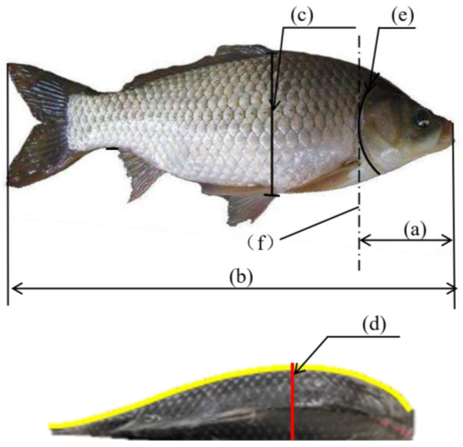
2.3.1. Feature Extraction
2.3.2. Establishment of Fish Head Cut Position Identification Models
LS-SVM Model
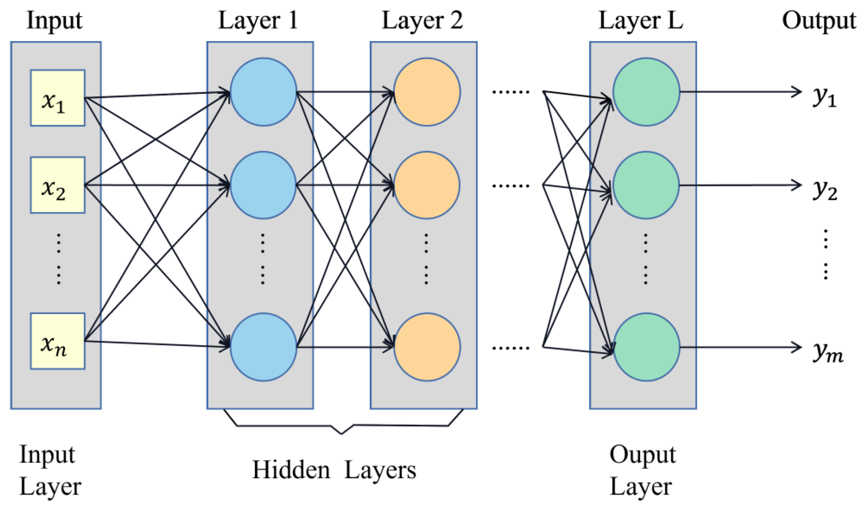
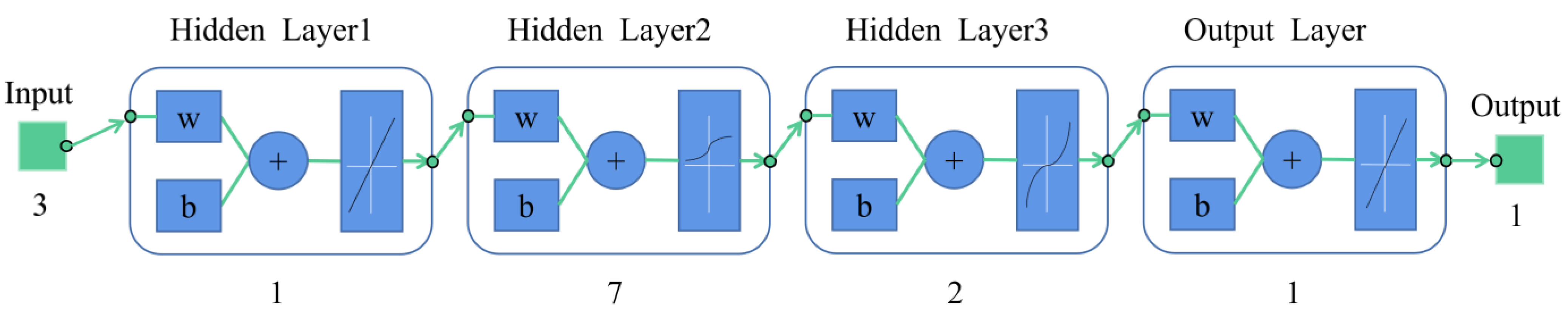
PSO-BP Model
LSTM Model
2.4. Model Evaluation Metrics
3. Results
3.1. Data Pre-Processing
3.1.1. Data Segmentation
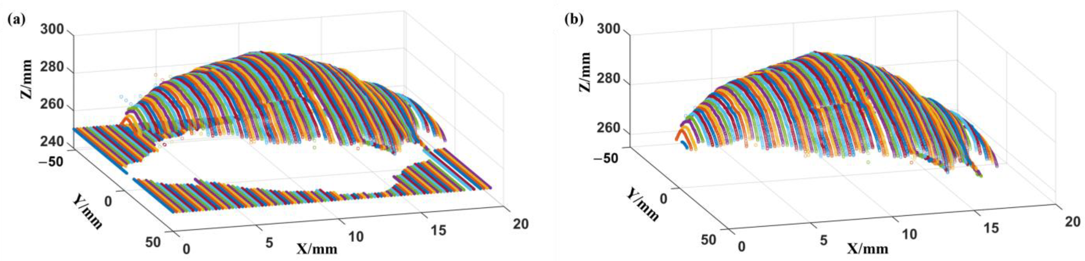
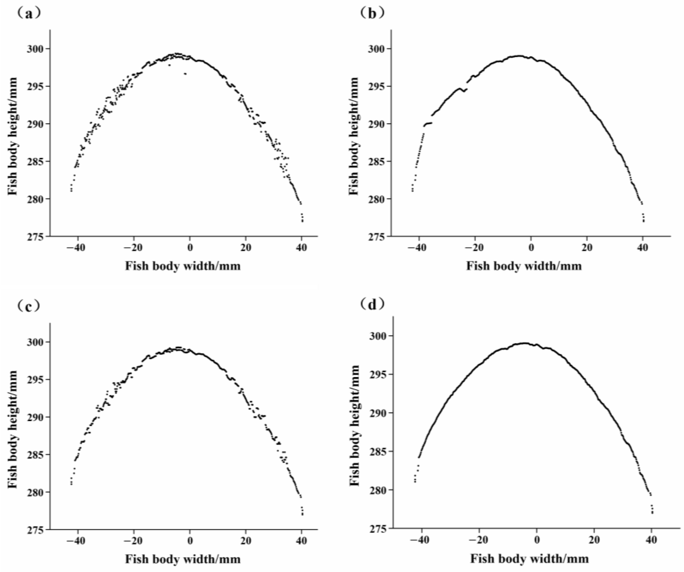
3.1.2. Data Filtering
3.2. Fish Head Cut Position Identification
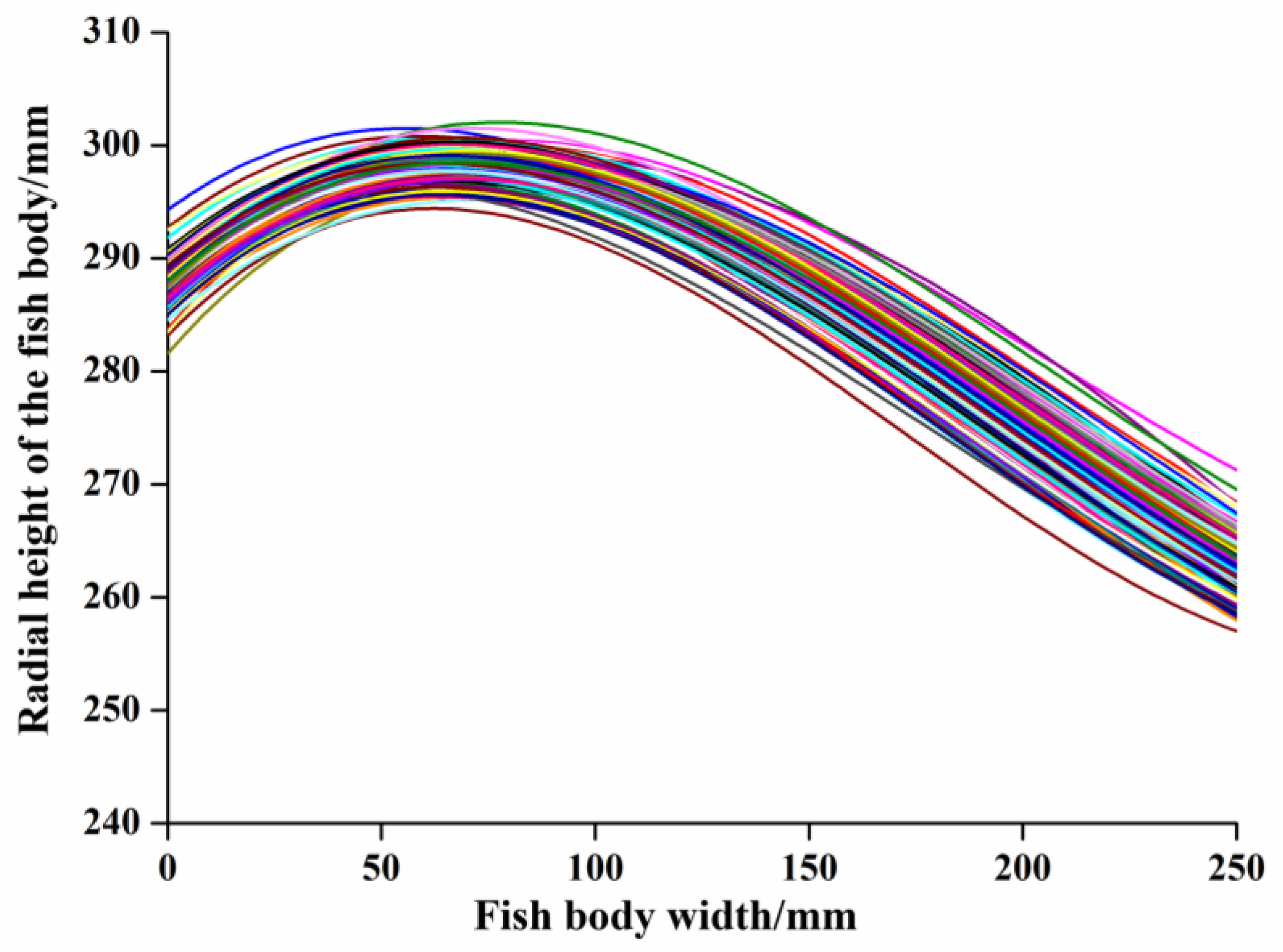
3.2.1. Extraction of Ventral–Dorsal Demarcation Line
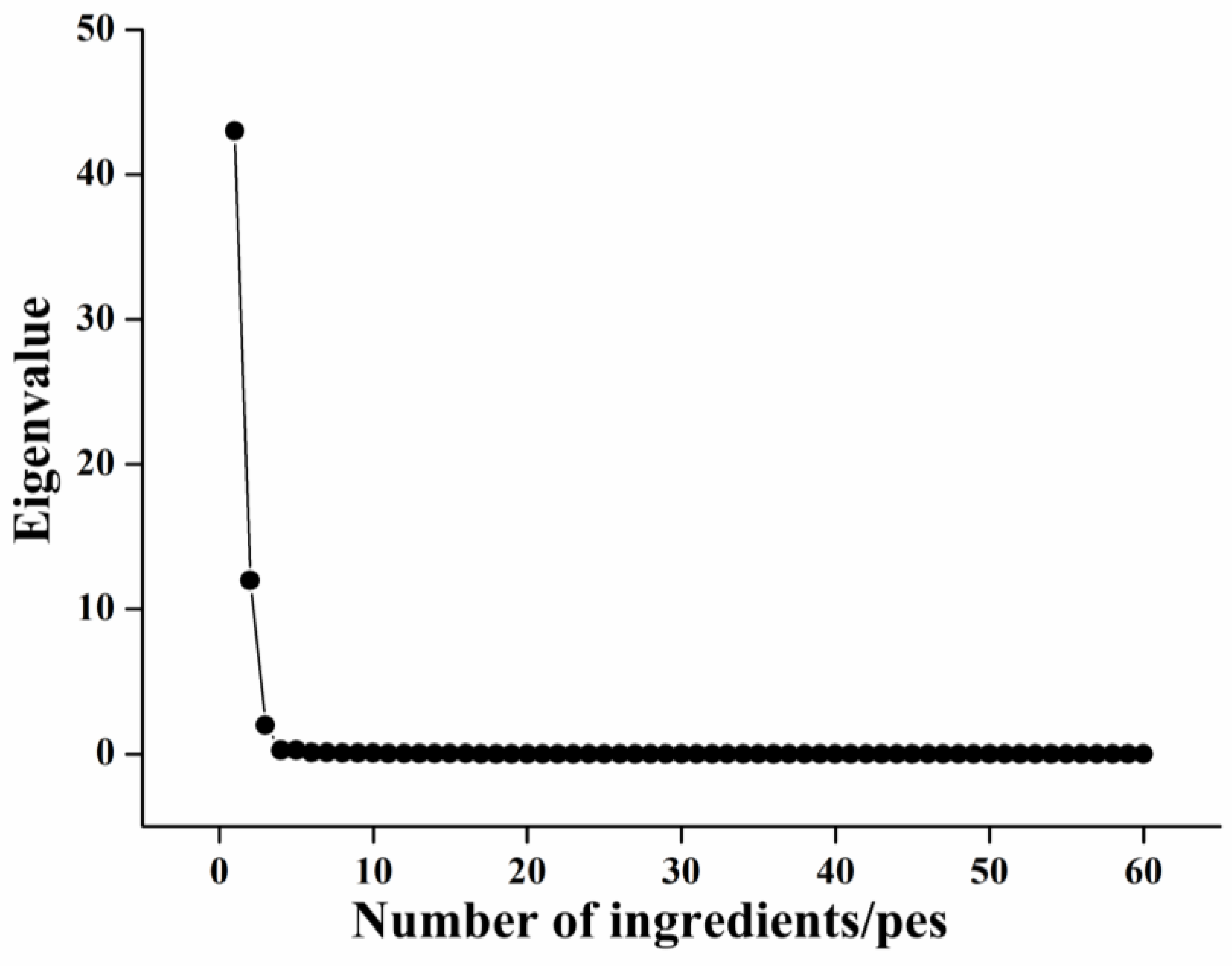
3.2.2. Data Dimensionality Reduction of Abdominal and Dorsal Dividing Lines
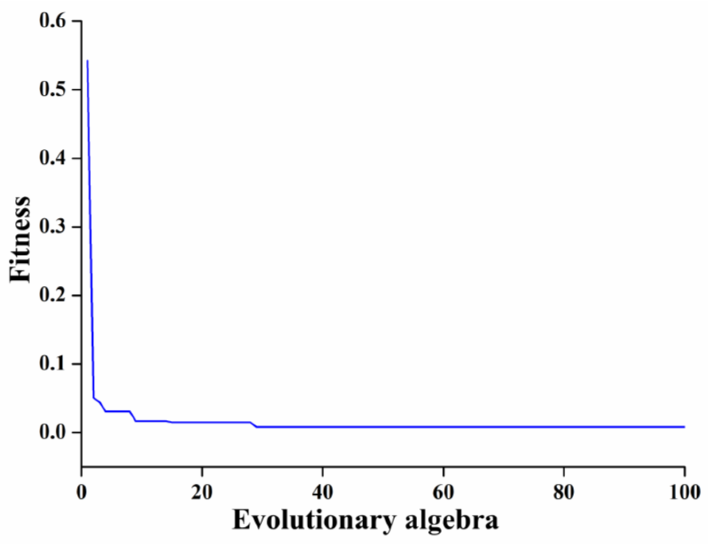
3.2.3. Fish Head Cutting Position Identification Model
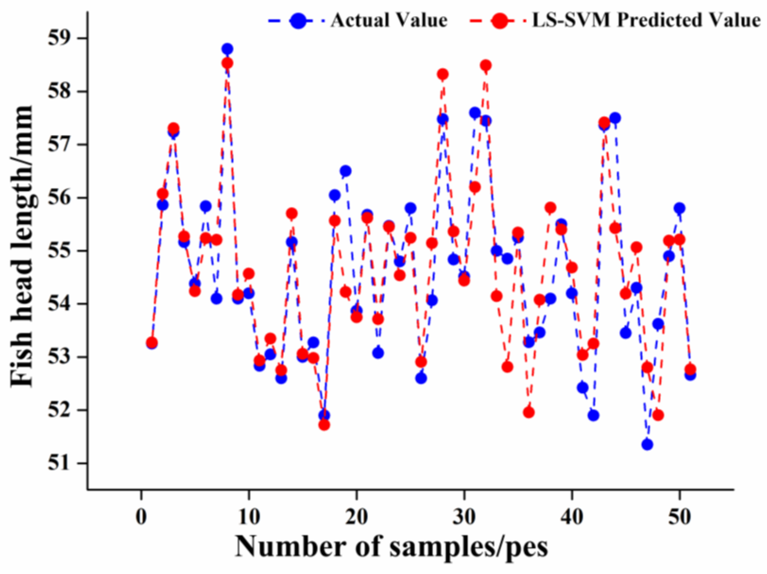
LS-SVM Model
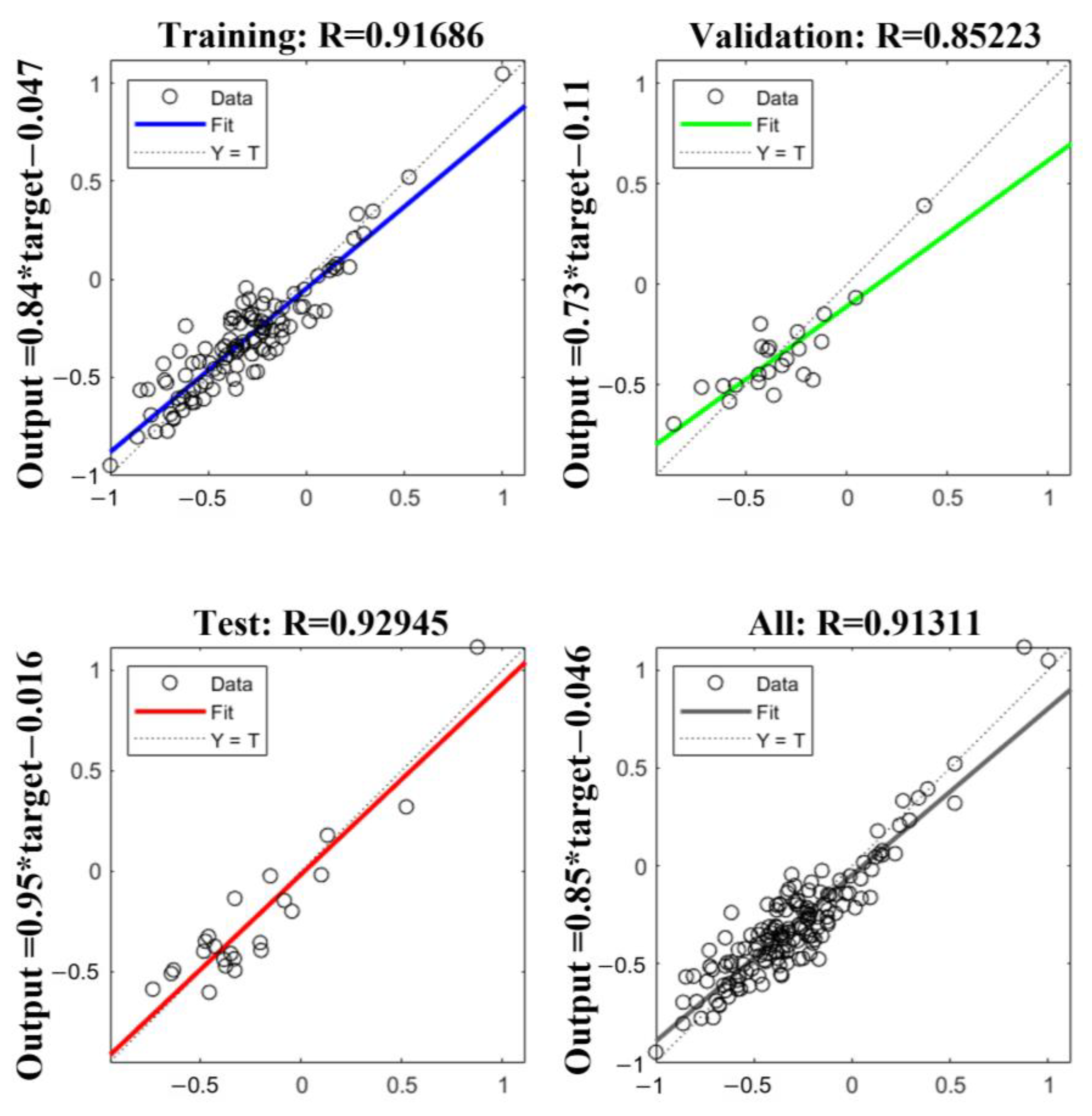
PSO-BP Model
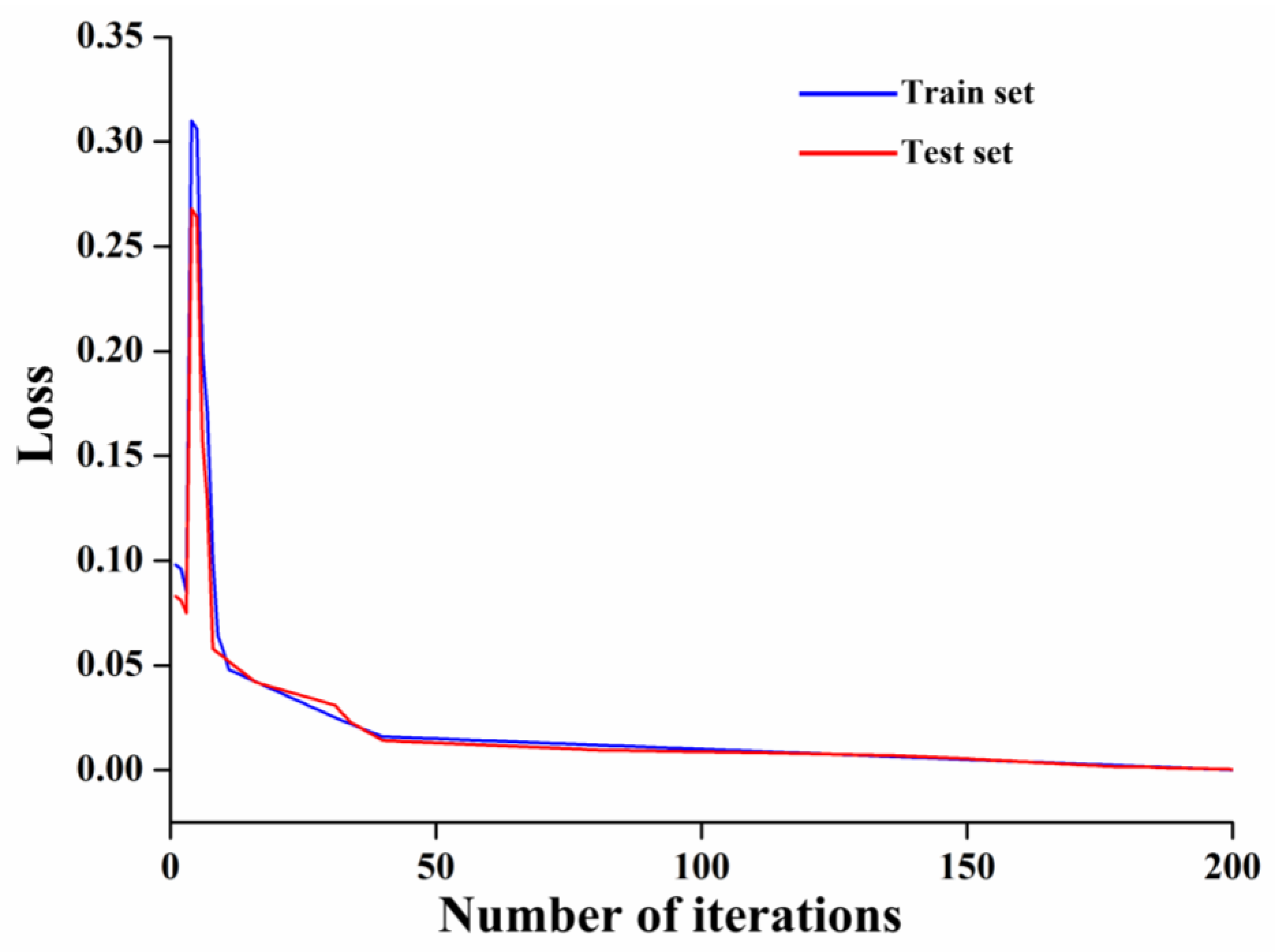
LSTM Model
4. Conclusions
Author Contributions
Funding
Data Availability Statement
Conflicts of Interest
References
- Azarmdel, H.; Mohtasebi, S.S.; Jafari, A.; Muñoz, A.R. Developing an orientation and cutting point determination algorithm for a trout fish processing system using machine vision. Comput. Electron. Agric. 2019, 162, 613–629. [Google Scholar] [CrossRef]
- Qing, C.; Branch, D. Method study on mechanized head cutting for marine small fish. Fish. Mod. 2012, 39, 38–42. [Google Scholar]
- Wang, H.H.; Zhang, X.Y.; Li, P.P.; Sun, J.L.; Yan, P.T.; Zhang, X.; Liu, Y.Q. A New Approach for Unqualified Salted Sea Cucumber Identification: Integration of Image Texture and Machine Learning under the Pressure Contact. J. Sens. 2020, 2020, 8834614. [Google Scholar] [CrossRef]
- Mustafa, A.; Volino, M.; Kim, H.; Guillemaut, J.-Y.; Hilton, A. Temporally Coherent General Dynamic Scene Reconstruction. Int. J. Comput. Vis. 2021, 129, 123–141. [Google Scholar] [CrossRef]
- Wang, J.H.; Yang, Y.X.; Zhou, Y.G. Dynamic Three-Dimensional Surface Reconstruction Approach for Continuously Deformed Objects. IEEE Photonics J. 2021, 13, 1–15. [Google Scholar] [CrossRef]
- Liu, Z.; Xiang, C.Q.; Chen, T. Automated Binocular Vision Measurement of Food Dimensions and Volume for Dietary Evaluation. Comput. Sci. Eng. 2018. Available online: https://ieeexplore.ieee.org/abstract/document/8365083 (accessed on 13 December 2023).
- Tsoulias, N.; Xanthopoulos, G.; Fountas, S.; Zude, M. In-situ detection of apple fruit using a 2D LiDAR laser scanner. In Proceedings of the IEEE International Workshop on Metrology for Agriculture and Forestry, Trento, Italy, 4–6 November 2020. [Google Scholar]
- Antequera, T.; Caballero, D.; Grassi, S.; Uttaro, B.; Perez-Palacios, T. Evaluation of fresh meat quality by Hyperspectral Imaging (HSI), Nuclear Magnetic Resonance (NMR) and Magnetic Resonance Imaging (MRI): A review. Meat Sci. 2020, 172, 108340. [Google Scholar] [CrossRef] [PubMed]
- Ando, M.; Sugiyama, H.; Maksimenko, A.; Rubenstein, E.; Roberson, J.; Shimao, D.; Hashimoto, E.; Mori, K. X-ray dark-field imaging and its application to medicine. Radiat. Phys. Chem. 2004, 71, 899–904. [Google Scholar] [CrossRef]
- Weisgerber, J.N.; Medill, S.A.; McLoughlin, P.D. Parallel-Laser Photogrammetry to Estimate Body Size in Free-Ranging Mammals. Wildl. Soc. Bull. 2015, 39, 422–428. [Google Scholar] [CrossRef]
- Chen, H.; Liu, Z.; Gu, J.; Ai, W.; Wen, J.; Cai, K. Quantitative analysis of soil nutrition based on FT-NIR spectroscopy integrated with BP neural deep learning. Anal. Methods 2018, 10, 5004–5013. [Google Scholar] [CrossRef]
- Cobourn, W.G.; Dolcine, L.; French, M.; Hubbard, M.C. A comparison of nonlinear regression and neural network models for ground-level ozone forecasting. Air Repair 2000, 50, 1999–2009. [Google Scholar] [CrossRef] [PubMed]
- Lin, W.M.; Tu, C.S.; Yang, R.F.; Tsai, M.T. Particle swarm optimisation aided least-square support vector machine for load forecast with spikes. Iet Gener. Transm. Distrib. 2016, 10, 1145–1153. [Google Scholar] [CrossRef]
- Zhu, F.L.; He, Y.; Shao, Y.N. Application of Near-Infrared Hyperspectral Imaging to Predicting Water Content in Salmon Flesh. Spectrosc. Spectr. Anal. 2015, 35, 113–117. [Google Scholar]
- Zhang, Y.; Jia, S.; Zhang, W. Predicting acetic acid content in the final beer using neural networks and support vector machine. J. Inst. Brew. 2012, 118, 361–367. [Google Scholar] [CrossRef]
- Khoshnoudi-Nia, S.; Moosavi-Nasab, M. Nondestructive Determination of Microbial, Biochemical, and Chemical Changes in Rainbow Trout (Oncorhynchus mykiss) During Refrigerated Storage Using Hyperspectral Imaging Technique. Food Anal. Methods 2019, 12, 1635–1647. [Google Scholar] [CrossRef]
- Wang, F.R.; Xie, B.M.; Lue, E.L.; Zeng, Z.X.; Mei, S.; Ma, C.Y.; Guo, J.M. Design of a Moisture Content Detection System for Yinghong No. 9 Tea Leaves Based on Machine Vision. Appl. Sci. 2023, 13, 1806. [Google Scholar] [CrossRef]
- Deng, Y.; Xiao, H.J.; Xu, J.X.; Wang, H. Prediction model of PSO-BP neural network on coliform amount in special food. Saudi J. Biol. Sci. 2019, 26, 1154–1160. [Google Scholar] [CrossRef] [PubMed]
- Zhang, L.; Liu, J.; Zhi, L. Research on Grain Yield Prediction Method Based on Improved PSO-BP. J. Appl. Sci. 2014, 14, 1990–1995. [Google Scholar] [CrossRef]
- Örnek, M.N.; Örnek, H.K. Developing a deep neural network model for predicting carrots volume. J. Food Meas. Charact. 2021, 15, 3471–3479. [Google Scholar] [CrossRef]
- Zhong, N.; Li, Y.P.; Li, X.Z.; Guo, C.X.; Wu, T. Accurate prediction of salmon storage time using improved Raman spectroscopy. J. Food Eng. 2021, 293, 110378. [Google Scholar] [CrossRef]
- Gao, C.; Bao, S.; Zhou, C.; He, X.; Shiju, E.; Sun, J.; Gong, J. Research on the line point cloud processing method for railway wheel profile with a laser profile sensor. Measurement 2023, 211, 112640. [Google Scholar] [CrossRef]
- Zabalza, J.; Ren, J.; Ren, J.; Liu, Z.; Marshall, S. Structured covariance principal component analysis for real-time onsite feature extraction and dimensionality reduction in hyperspectral imaging. Appl. Opt. 2014, 53, 4440–4449. [Google Scholar] [CrossRef] [PubMed]
- Zhang, X.L.; Liu, F.; He, Y.; Li, X.L. Application of Hyperspectral Imaging and Chemometric Calibrations for Variety Discrimination of Maize Seeds. Sensors 2012, 12, 17234–17246. [Google Scholar] [CrossRef] [PubMed]
- Tarhouni, M.; Laabidi, K.; Lahmari-Ksouri, M.; Zidi, S. System Identification based on Multi-kernel Least Squares Support Vector Machines (Multi-kernel LS-SVM). In Proceedings of the International Joint Conference on Computational Intelligence, Dhaka, Bangladesh, 14–15 December 2018. [Google Scholar]
- Zhang, X.; Sun, J.L.; Li, P.P.; Zeng, F.Y.; Wang, H.H. Hyperspectral detection of salted sea cucumber adulteration using different spectral preprocessing techniques and SVM method. Lwt-Food Sci. Technol. 2021, 152, 112295. [Google Scholar] [CrossRef]
- Wang, J.; Si, H.P.; Gao, Z.; Shi, L. Winter Wheat Yield Prediction Using an LSTM Model from MODIS LAI Products. Agriculture 2022, 12, 1707. [Google Scholar] [CrossRef]
- Qi, J.; Du, J.; Siniscalchi, S.M.; Ma, X.L.; Lee, C.H. Analyzing Upper Bounds on Mean Absolute Errors for Deep Neural Network-Based Vector-to-Vector Regression. IEEE Trans. Signal Process. 2020, 68, 3411–3422. [Google Scholar] [CrossRef]
- Weijie, W.; Yanmin, L. Analysis of the Mean Absolute Error (MAE) and the Root Mean Square Error (RMSE) in Assessing Rounding Model. In OP Conference Series: Materials Science and Engineering; IOP Publishing: Bristol, UK, 2018; p. 012049. [Google Scholar]
- Cheng, J.H.; Sun, D.W.; Pu, H.B.; Zhu, Z.W. Development of hyperspectral imaging coupled with chemometric analysis to monitor K value for evaluation of chemical spoilage in fish fillets. Food Chem. 2015, 185, 245–253. [Google Scholar] [CrossRef]
- Khoshnoudi-Nia, S.; Moosavi-Nasab, M. Prediction of various freshness indicators in fish fillets by one multispectral imaging system. Sci. Rep. 2019, 9, 14704. [Google Scholar] [CrossRef]


| Sample Size | Statistical Indicator | a/mm | b/mm | c/mm | d/mm | Weight/g |
|---|---|---|---|---|---|---|
| 204 | Maximum value | 63.1 | 239.4 | 103.7 | 51.54 | 569 |
| Minimum value | 50.1 | 200.8 | 94.6 | 45.3 | 473 | |
| Mean | 223.6 | 54.6 | 100.9 | 47.49 | 532.1 | |
| Standard deviation | 2.5 | 8.9 | 2.2 | 1.85 | 21.6 |
| Component | Initial Eigenvalue | Extraction of Squares and Loading | Rotate the Square and Load | ||||||
|---|---|---|---|---|---|---|---|---|---|
| Total | Variance of % | Cumulative % | Total | Variance of % | Cumulative % | Total | Variance of % | Cumulative % | |
| 1 | 43.031 | 71.718 | 71.718 | 43.031 | 71.718 | 71.718 | 34.740 | 57.901 | 57.901 |
| 2 | 11.990 | 19.983 | 91.702 | 11.990 | 19.983 | 91.702 | 16.894 | 28.157 | 86.058 |
| 3 | 1.999 | 3.3319 | 95.033 | 1.999 | 3.331 | 95.033 | 5.385 | 8.974 | 95.033 |
| 4 | 0.842 | 1.403 | 96.436 | ||||||
| 5 | 0.386 | 0.643 | 97.079 | ||||||
| 6 | 0.340 | 0.567 | 97.646 | ||||||
| 7 | 0.261 | 0.434 | 98.080 | ||||||
| 8 | 0.139 | 0.232 | 98.312 | ||||||
| 9 | 0.112 | 0.187 | 98.496 | ||||||
| 10 | 0.097 | 0.161 | 98.661 | ||||||
| ...... | |||||||||
| 204 | −1.04 × 10⁻¹⁵ | −1.74 × 10⁻¹⁵ | 100.00 | ||||||
Disclaimer/Publisher’s Note: The statements, opinions and data contained in all publications are solely those of the individual author(s) and contributor(s) and not of MDPI and/or the editor(s). MDPI and/or the editor(s) disclaim responsibility for any injury to people or property resulting from any ideas, methods, instructions or products referred to in the content. |
© 2023 by the authors. Licensee MDPI, Basel, Switzerland. This article is an open access article distributed under the terms and conditions of the Creative Commons Attribution (CC BY) license (https://creativecommons.org/licenses/by/4.0/).
Share and Cite
Zhang, X.; Gong, Z.; Liang, X.; Sun, W.; Ma, J.; Wang, H. Line Laser Scanning Combined with Machine Learning for Fish Head Cutting Position Identification. Foods 2023, 12, 4518. https://doi.org/10.3390/foods12244518
Zhang X, Gong Z, Liang X, Sun W, Ma J, Wang H. Line Laser Scanning Combined with Machine Learning for Fish Head Cutting Position Identification. Foods. 2023; 12(24):4518. https://doi.org/10.3390/foods12244518
Chicago/Turabian StyleZhang, Xu, Ze Gong, Xinyu Liang, Weichen Sun, Junxiao Ma, and Huihui Wang. 2023. "Line Laser Scanning Combined with Machine Learning for Fish Head Cutting Position Identification" Foods 12, no. 24: 4518. https://doi.org/10.3390/foods12244518
APA StyleZhang, X., Gong, Z., Liang, X., Sun, W., Ma, J., & Wang, H. (2023). Line Laser Scanning Combined with Machine Learning for Fish Head Cutting Position Identification. Foods, 12(24), 4518. https://doi.org/10.3390/foods12244518