
Meta-Learning for Few-Shot Plant Disease Detection


Abstract
:1. Introduction
2. Materials and Methods
2.1. Datasets
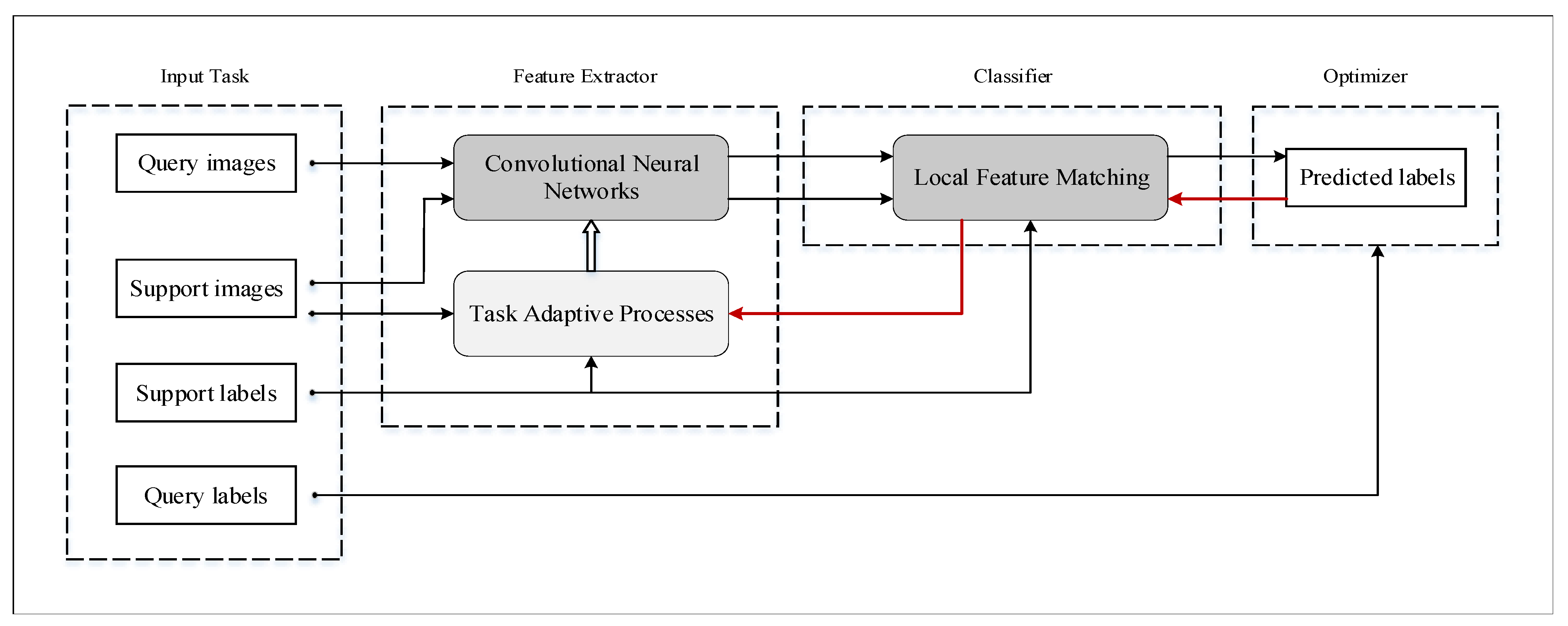
2.2. LFM-CNAPS
2.2.1. Task
2.2.2. Conditional Adaptive Feature Extractor
2.2.3. Local Feature Matching Classifier
2.2.4. Parameters Optimizer
2.3. Task Activation Mapping
3. Results
3.1. Performance of Plant Disease Detection
3.2. Visual Explanations
4. Discussion
5. Conclusions
Author Contributions
Funding
Institutional Review Board Statement
Informed Consent Statement
Data Availability Statement
Conflicts of Interest
References
- Muimba-Kankolongo, A. Food Crop Production by Smallholder Farmers in Southern Africa || Climates and Agroecologies; Academic Press: Cambridge, MA, USA, 2018; pp. 5–13. [Google Scholar]
- Ferentinos, K.P. Deep learning models for plant disease detection and diagnosis. Comput. Electron. Agric. 2018, 145, 311–318. [Google Scholar] [CrossRef]
- Mohameth, F.; Bingcai, C.; Sada, K.A. Plant disease detection with deep learning and feature extraction using plant village. J. Comput. Commun. 2020, 8, 10–22. [Google Scholar] [CrossRef]
- Klauser, D. Challenges in monitoring and managing plant diseases in developing countries. J. Plant Dis. Prot. 2018, 125, 235–237. [Google Scholar] [CrossRef]
- Kader, A.A.; Kasmire, R.F.; Reid, M.S.; Sommer, N.F.; Thompson, J.F. Postharvest Technology of Horticultural Crops; University of California Agriculture and Natural Resources: Davis, CA, USA, 2002. [Google Scholar]
- Teng, P.S.; James, W.C. Disease and yield loss assessment. In Plant Pathologists Pocketbook; CABI: Wallingford, UK, 2002. [Google Scholar]
- Maxwell, S. Food security: A post-modern perspective. Food Policy 1996, 21, 155–170. [Google Scholar] [CrossRef] [Green Version]
- Hunter, M.C.; Smith, R.G.; Schipanski, M.E.; Atwood, L.W.; Mortensen, D.A. Agriculture in 2050: Recalibrating targets for sustainable intensification. Bioscience 2017, 67, 386–391. [Google Scholar] [CrossRef] [Green Version]
- Fang, Y.; Ramasamy, R.P. Current and prospective methods for plant disease detection. Biosensors 2015, 5, 537–561. [Google Scholar] [CrossRef] [PubMed] [Green Version]
- Sharma, P.; Berwal, Y.P.S.; Ghai, W. Performance analysis of deep learning CNN models for disease detection in plants using image segmentation. Inf. Process. Agric. 2020, 7, 566–574. [Google Scholar] [CrossRef]
- Taheri-Garavand, A.; Nejad, A.R.; Fanourakis, D.; Fatahi, S.; Majd, M.A. Employment of artificial neural networks for non-invasive estimation of leaf water status using color features: A case study in Spathiphyllum wallisii. Acta Physiol. Plant. 2021, 43, 1–11. [Google Scholar] [CrossRef]
- LeCun, Y.; Bengio, Y. Convolutional networks for images, speech, and time series. Handb. Brain Theory Neural Netw. 1995, 3361, 1995. [Google Scholar]
- LeCun, Y.; Bengio, Y.; Hinton, G. Deep learning. Nature 2015, 521, 436–444. [Google Scholar] [CrossRef]
- Li, W.; Xu, L.; Liang, Z.; Wang, S.; Cao, J.; Lam, T.C.; Cui, X. JDGAN: Enhancing generator on extremely limited data via joint distribution. Neurocomputing 2021, 431, 148–162. [Google Scholar] [CrossRef]
- Li, W.; Fan, L.; Wang, Z.; Ma, C.; Cui, X. Tackling mode collapse in multi-generator GANs with orthogonal vectors. Pattern Recognit. 2021, 110, 107646. [Google Scholar] [CrossRef]
- Taheri-Garavand, A.; Nasiri, A.; Fanourakis, D.; Fatahi, S.; Omid, M.; Nikoloudakis, N. Automated In Situ Seed Variety Identification via Deep Learning: A Case Study in Chickpea. Plants 2021, 10, 1406. [Google Scholar] [CrossRef]
- Nasiri, A.; Taheri-Garavand, A.; Fanourakis, D.; Zhang, Y.D.; Nikoloudakis, N. Automated Grapevine Cultivar Identification via Leaf Imaging and Deep Convolutional Neural Networks: A Proof-of-Concept Study Employing Primary Iranian Varieties. Plants 2021, 10, 1628. [Google Scholar] [CrossRef] [PubMed]
- Hughes, D.; Salathé, M. An open access repository of images on plant health to enable the development of mobile disease diagnostics. arXiv 2015, arXiv:1511.08060. [Google Scholar]
- Strange, R.N.; Scott, P.R. Plant disease: A threat to global food security. Annu. Rev. Phytopathol. 2005, 43, 83–116. [Google Scholar] [CrossRef] [PubMed]
- Vilalta, R.; Drissi, Y. A perspective view and survey of meta-learning. Artif. Intell. Rev. 2002, 18, 77–95. [Google Scholar] [CrossRef]
- Vanschoren, J. Meta-learning: A survey. arXiv 2018, arXiv:1810.03548. [Google Scholar]
- Pan, S.J.; Qiang, Y. A Survey on Transfer Learning. IEEE Trans. Knowl. Data Eng. 2010, 22, 1345–1359. [Google Scholar] [CrossRef]
- Snell, J.; Swersky, K.; Zemel, R.S. Prototypical networks for few-shot learning. arXiv 2017, arXiv:1703.05175. [Google Scholar]
- Requeima, J.; Gordon, J.; Bronskill, J.; Nowozin, S.; Turner, R.E. Fast and flexible multi-task classification using conditional neural adaptive processes. Adv. Neural Inf. Process. Syst. 2019, 32, 7959–7970. [Google Scholar]
- Bateni, P.; Goyal, R.; Masrani, V.; Wood, F.; Sigal, L. Improved few-shot visual classification. In Proceedings of the IEEE/CVF Conference on Computer Vision and Pattern Recognition, Seattle, WA, USA, 13–19 June 2020; pp. 14493–14502. [Google Scholar]
- Lin, X.; Ye, M.; Gong, Y.; Buracas, G.; Basiou, N.; Divakaran, A.; Yao, Y. Modular Adaptation for Cross-Domain Few-Shot Learning. arXiv 2021, arXiv:2104.00619. [Google Scholar]
- Cai, J.; Shen, S.M. Cross-domain few-shot learning with meta fine-tuning. arXiv 2020, arXiv:2005.10544. [Google Scholar]
- Davis, J.V.; Kulis, B.; Jain, P.; Sra, S.; Dhillon, I.S. Information-theoretic metric learning. In Proceedings of the 24th International Conference on Machine Learning, Corvallis, OR, USA, 20–24 June 2007; pp. 209–216. [Google Scholar]
- Vinyals, O.; Blundell, C.; Lillicrap, T.; Wierstra, D. Matching networks for one shot learning. Adv. Neural Inf. Process. Syst. 2016, 29, 3630–3638. [Google Scholar]
- Triantafillou, E.; Zhu, T.; Dumoulin, V.; Lamblin, P.; Evci, U.; Xu, K.; Goroshin, R.; Gelada, C.; Swersky, K.; Manzagol, P.A.; et al. Meta-dataset: A dataset of datasets for learning to learn from few examples. arXiv 2019, arXiv:1903.03096. [Google Scholar]
- Russakovsky, O.; Deng, J.; Su, H.; Krause, J.; Satheesh, S.; Ma, S.; Huang, Z.; Karpathy, A.; Khosla, A.; Bernstein, M.; et al. Imagenet large scale visual recognition challenge. Int. J. Comput. Vis. 2015, 115, 211–252. [Google Scholar] [CrossRef] [Green Version]
- Lake, B.M.; Salakhutdinov, R.; Tenenbaum, J.B. Human-level concept learning through probabilistic program induction. Science 2015, 350, 1332–1338. [Google Scholar] [CrossRef] [Green Version]
- Maji, S.; Rahtu, E.; Kannala, J.; Blaschko, M.; Vedaldi, A. Fine-grained visual classification of aircraft. arXiv 2013, arXiv:1306.5151. [Google Scholar]
- Wah, C.; Branson, S.; Welinder, P.; Perona, P.; Belongie, S. The Caltech-Ucsd Birds-200-2011 Dataset; California Institute of Technology: Pasadena, CA, USA, 2011. [Google Scholar]
- Cimpoi, M.; Maji, S.; Kokkinos, I.; Mohamed, S.; Vedaldi, A. Describing textures in the wild. In Proceedings of the IEEE Conference on Computer Vision and Pattern Recognition, Columbus, OH, USA, 23–28 June 2014; pp. 3606–3613. [Google Scholar]
- Wheatley, G. Quick Draw; Mathematics Learning: Bethany Beach, DE, USA, 2007. [Google Scholar]
- Schroeder, B.; Cui, Y. Fgvcx Fungi Classification Challenge 2018. Available online: github.com/visipedia/fgvcx_fungi_comp (accessed on 14 July 2021).
- Nilsback, M.E.; Zisserman, A. Automated flower classification over a large number of classes. In Proceedings of the 2008 Sixth Indian Conference on Computer Vision, Graphics & Image Processing, Bhubaneswar, India, 16–19 December 2008; pp. 722–729. [Google Scholar]
- Houben, S.; Stallkamp, J.; Salmen, J.; Schlipsing, M.; Igel, C. Detection of traffic signs in real-world images: The German Traffic Sign Detection Benchmark. In Proceedings of the 2013 International Joint Conference on Neural Networks (IJCNN), Dallas, TX, USA, 4–9 August 2013; pp. 1–8. [Google Scholar]
- Lin, T.Y.; Maire, M.; Belongie, S.; Hays, J.; Perona, P.; Ramanan, D.; Dollár, P.; Zitnick, C.L. Microsoft coco: Common objects in context. In Proceedings of the European Conference on Computer Visio, Zurich, Switzerland, 6–12 September 2014; pp. 740–755. [Google Scholar]
- Thapa, R.; Zhang, K.; Snavely, N.; Belongie, S.; Khan, A. The Plant Pathology Challenge 2020 data set to classify foliar disease of apples. Appl. Plant Sci. 2020, 8, e11390. [Google Scholar] [CrossRef]
- He, K.; Zhang, X.; Ren, S.; Sun, J. Deep residual learning for image recognition. In Proceedings of the IEEE Conference on Computer Vision and Pattern Recognition, Las Vegas, NV, USA, 27–30 June 2016; pp. 770–778. [Google Scholar]
- Finn, C.; Abbeel, P.; Levine, S. Model-agnostic meta-learning for fast adaptation of deep networks. In Proceedings of the International Conference on Machine Learning, PMLR, Sydney, Australia, 6–11 August 2017; pp. 1126–1135. [Google Scholar]
- Perez, E.; Strub, F.; De Vries, H.; Dumoulin, V.; Courville, A. Film: Visual reasoning with a general conditioning layer. In Proceedings of the AAAI Conference on Artificial Intelligence, New Orleans, LA, USA, 2–7 February 2018; Volume 32. [Google Scholar]
- Li, W.; Liu, X.; Liu, J.; Chen, P.; Wan, S.; Cui, X. On improving the accuracy with auto-encoder on conjunctivitis. Appl. Soft Comput. 2019, 81, 105489. [Google Scholar] [CrossRef]
- Joachims, T. Making Large-Scale SVM Learning Practical. Technical Report. 1998. Available online: https://www.econstor.eu/handle/10419/77178 (accessed on 9 March 2021).
- Li, W.; Wang, L.; Xu, J.; Huo, J.; Gao, Y.; Luo, J. Revisiting local descriptor based image-to-class measure for few-shot learning. In Proceedings of the IEEE/CVF Conference on Computer Vision and Pattern Recognition, Long Beach, CA, USA, 15–20 June 2019; pp. 7260–7268. [Google Scholar]
- Zhang, Z.; Sabuncu, M.R. Generalized cross entropy loss for training deep neural networks with noisy labels. In Proceedings of the 32nd Conference on Neural Information Processing Systems (NeurIPS), Montreal, QC, Canada, 3–8 December 2018. [Google Scholar]
- Kingma, D.P.; Ba, J. Adam: A method for stochastic optimization. arXiv 2014, arXiv:1412.6980. [Google Scholar]
- Selvaraju, R.R.; Cogswell, M.; Das, A.; Vedantam, R.; Parikh, D.; Batra, D. Grad-cam: Visual explanations from deep networks via gradient-based localization. In Proceedings of the IEEE International Conference on Computer Vision, Venice, Italy, 22–29 October 2017; pp. 618–626. [Google Scholar]
- Chatzistathis, T.; Fanourakis, D.; Aliniaeifard, S.; Kotsiras, A.; Delis, C.; Tsaniklidis, G. Leaf Age-Dependent Effects of Boron Toxicity in Two Cucumis melo Varieties. Agronomy 2021, 11, 759. [Google Scholar] [CrossRef]
- Taheri-Garavand, A.; Mumivand, H.; Fanourakis, D.; Fatahi, S.; Taghipour, S. An artificial neural network approach for non-invasive estimation of essential oil content and composition through considering drying processing factors: A case study in Mentha aquatica. Ind. Crop. Prod. 2021, 171, 113985. [Google Scholar] [CrossRef]


| Name | Value |
|---|---|
| Video Memory | 11G |
| Graphics | NVIDIA GeForce GTX 1080 Ti |
| Processor | Intel(R) Xeon(R) CPU E5-2640 |
| Operating system | Windows 10 Home 64 |
| Training time | 17,548.73 s |
| Test time | 57.36 s |
| Dataset Name | Accuracy (%) |
|---|---|
| ilsvrc 2012 | 55.0+/−1.0 |
| omniglot | 92.0+/−0.6 |
| aircraft | 82.4+/−0.6 |
| cu birds | 74.3+/−0.8 |
| dtd | 65.3+/−0.7 |
| quickdraw | 75.5+/−0.8 |
| fungi | 48.0+/−1.1 |
| Vgg flower | 89.4+/−0.5 |
| Traffic sign | 68.2+/−0.7 |
| mscoco | 51.1+/−1.0 |
| mnist | 93.3+/−0.4 |
| cifar10 | 71.1+/−0.7 |
| cifar100 | 57.3+/−1.0 |
| Species | Number of Plant Diseases | Number of Samples |
|---|---|---|
| Apple foliar disease | ||
| Alstonia Scholaris | 2 | 433 |
| Arjun | 2 | 452 |
| Bael | 2 | 266 |
| Chinar | 2 | 223 |
| Gauva | 2 | 419 |
| Jamun | 2 | 624 |
| Jatropha | 2 | 257 |
| Lemon | 2 | 236 |
| PlantVillage | ||
| Apple | 4 | 7169 |
| Blueberry | 1 | 1816 |
| Cherry | 2 | 3509 |
| Corn | 4 | 7316 |
| Grape | 4 | 7222 |
| Orange | 1 | 2010 |
| Peach | 2 | 3566 |
| Pepper | 2 | 3901 |
| Potato | 2 | 3763 |
| Tomato | 10 | 18,345 |
| Number of training steps | Training accuracy (%) | |
| 10,000 | 97.0 | |
| 20,000 | 97.5 | |
| Plant State | Number of Samples |
| Mango diseased | 265 |
| Mango healthy | 170 |
| Pomegranate diseased | 272 |
| Pomegranate healthy | 287 |
| Pongamia Pinnata diseased | 276 |
| Pongamia Pinnata healthy | 322 |
| Potato Late blight | 1939 |
| Raspberry healthy | 1781 |
| Soybean healthy | 2022 |
| Squash Powdery mildew | 1736 |
| Strawberry healthy | 1824 |
| Strawberry Leaf scorch | 1774 |
| Method | Accuracy (%) |
| RESNET18 + FC | 20.0+/−0.5 |
| MatchingNet | 19.5+/−0.5 |
| ProtoNet | 20.5+/−0.6 |
| RESNET18 + LFM | 85.2+/−0.7 |
| Simple-CNAPS | 92.5+/−0.4 |
| Meta Fine-Tuning | 91.14+/−0.5 |
| LFM-CNAPS | 93.9+/−0.4 |
| Feature Extractor | Classifier | Accuracy (%) |
|---|---|---|
| 20.0+/−0.5 | ||
| ✓ | 86.1+/−0.6 | |
| ✓ | 85.2+/−0.7 | |
| ✓ | ✓ | 93.9+/−0.4 |
| Plant Category | Number of Plant Diseases | Number of Samples |
| Apple | 4 | 1943 |
| Blueberry | 1 | 454 |
| Cherry | 2 | 877 |
| Corn | 4 | 1829 |
| Grape | 4 | 1805 |
| Orange | 1 | 503 |
| Peach | 2 | 891 |
| Pepper | 2 | 975 |
| Potato | 3 | 1426 |
| Raspberry | 1 | 445 |
| Soybean | 1 | 505 |
| Squash | 1 | 434 |
| Strawberry | 2 | 900 |
| Tomato | 10 | 4585 |
| Method | Test accuracy (%) | |
| RESNET18 + FC | 19.8+/−0.5 | |
| RESNET18 + LFM | 81.7+/−0.7 | |
| LFM-CNAPS | 89.0+/−0.5 | |
Publisher’s Note: MDPI stays neutral with regard to jurisdictional claims in published maps and institutional affiliations. |
© 2021 by the authors. Licensee MDPI, Basel, Switzerland. This article is an open access article distributed under the terms and conditions of the Creative Commons Attribution (CC BY) license (https://creativecommons.org/licenses/by/4.0/).
Share and Cite
Chen, L.; Cui, X.; Li, W. Meta-Learning for Few-Shot Plant Disease Detection. Foods 2021, 10, 2441. https://doi.org/10.3390/foods10102441
Chen L, Cui X, Li W. Meta-Learning for Few-Shot Plant Disease Detection. Foods. 2021; 10(10):2441. https://doi.org/10.3390/foods10102441
Chicago/Turabian StyleChen, Liangzhe, Xiaohui Cui, and Wei Li. 2021. "Meta-Learning for Few-Shot Plant Disease Detection" Foods 10, no. 10: 2441. https://doi.org/10.3390/foods10102441
APA StyleChen, L., Cui, X., & Li, W. (2021). Meta-Learning for Few-Shot Plant Disease Detection. Foods, 10(10), 2441. https://doi.org/10.3390/foods10102441