Abstract
Background: We studied in silico models of both organic and inorganic substances. In most cases, these in silico models are used for organic substances only. The following endpoints were taken for the case studies: the octanol–water coefficient (three models), the enthalpies of formation of organometallic compounds, and rat acute toxicity. Methods: The correlation weights were optimized using the Monte Carlo method with two special training and validation sets. The training set was structured into three subsets of active and passive training, as well as a calibration set. The division into these four subsets was carried out using the Las Vegas algorithm. It is assumed that considering groups of different splits into these four subsets is more informative than considering only a single split. Results: Models were built for the octanol–water coefficient for a set containing organic and inorganic substances or for a subset of the original data; other models were developed for a set containing only specially defined inorganic substances for platinum complexes. In addition, models of the enthalpy of formation and for toxicity in rats were built using the same approach for two sets of inorganic substances. Conclusions: A comparison of different methods for the optimization of correlation weights using the Monte Carlo method showed that optimization can be improved using the coefficient of conformism of a correlative prediction (CCCP) or the index of the ideality of correlation (IIC). Optimization with CCCP was the best option for the models of the octanol–water partition coefficient for the set of organic compounds, the octanol–water partition coefficient of the inorganic set, and the enthalpy of formation of the inorganic compounds. However, optimization with IIC was the best option in terms of the toxicity of the inorganic compounds in rats.
1. Introduction
It is generally accepted that the main difference between organic and inorganic chemistry lies in the composition of chemical compounds: organic chemistry studies compounds containing carbon atoms, often with complex and long chains (skeletons), while inorganic chemistry studies compounds that do not contain carbon atoms linked to hydrogen, with small structures that instead contain oxygen, nitrogen, sulfur, phosphorus, and metals. To proceed with the improvement of our knowledge, in many countries—Italy in particular—there are scientific associations (e.g., https://www.soc.chim.it/en, accessed 27 June 2025) that search for new technologies for applying chemistry to everyday life. Research groups from Italy, both individually and in co-operation with colleagues from other countries, are currently developing approaches to apply inorganic compounds in ecology [1,2,3], in medicine [4], and in various hybrid studies on well-known organic and inorganic compounds [5,6,7,8,9,10].
One of the most important fields of modern natural sciences is the development of in silico methods for the simulation of physicochemical and biochemical behaviors of organic and inorganic substances [11]. In terms of constructing quantitative structure–property/activity relationships (QSPRs/QSARs), organic substances [12,13,14,15,16,17,18,19] are a more common object of study compared to inorganic compounds [20,21,22,23]. The greater diversity of molecular structures for organic compounds, due to the possibility of the emergence of a huge number of variations in molecular architectures, provides the possibility of constructing and subsequently using databases in the format of molecular structure vectors of physicochemical and biochemical properties. The databases mentioned are necessary and are often required for successful QSPR/QSAR analysis [24,25,26,27]. Databases related to inorganic compounds are considerably modest in both their general number and contents [28,29]. However, it is obvious that knowledge related to both organic and inorganic compounds will never be exhaustive. In the case of both organic and inorganic compounds, concepts and algorithms for creating models of physicochemical and biochemical behavior are needed. Thus, from the very beginning of the discussed issue, it is possible to identify a simple difference in research works devoted to the QSPR/QSAR of organic and inorganic chemistry: there are a larger number of databases for the former and a smaller number of databases for the latter. In addition, there is an issue in the field of in silico methods regarding inorganic substances: by far, most models are related to organic substances, only using organometallic compounds in very few cases. Indeed, many models only use atoms commonly present in organic substances. Salts are disregarded and transformed into their neutral form. Indeed, salts are usually represented as a disconnected structure, with two separate parts, and this represents a complication for modeling in most cases. As a matter of fact, the most common software used to predict the properties of substances deals with organic substances and cannot be used for salts. Thus, this study wants to address this issue and at the same time explore the issues with modeling inorganic substances. Indeed, there may be other significant differences between the QSPR/QSAR of organic and that of inorganic compounds, but for this purpose, we need a system capable of coping with both inorganic and organic substances. Establishing such differences, as well as similarities between the QSPR/QSAR for organics and the QSPR/QSAR for inorganics, may be useful at least from a heuristic point of view. The aim of this study is therefore to examine how QSPR/QSAR models of organic and inorganic compounds obtained using stochastic approaches in models constructed by CORAL software (http://www.insilico.eu/coral, accessed 27 June 2025) may differ.
2. Results
2.1. QSPR Models for the Octanol–Water Partition Coefficient Observed for Dataset 1
This dataset contains both organic and inorganic substances. Descriptors of correlation weights (DCWs) are used to build up the models. The correlation weights were optimized using the index of ideality of correlation (IIC) in the case of the first target function (TF1) or the coefficient of conformism of a correlative prediction (CCCP) with the second target function (TF2). Three random splits (obtained with the Las Vegas algorithm) into an active training set, a passive training set, a calibration set, and an external (invisible) validation set were studied.
Compounds of the active training set represented via a simplified molecular input line entry system (SMILES) were the basis for the optimization of correlation weights. The SMILES of the passive training set allows us to estimate how suitable the obtained correlation weights are for compounds not involved in the optimization process. The SMILES of the calibration set aims to catch the start of stagnation (situations when changes in correlation weights are no longer accompanied by changes in the statistical quality of the model on the calibration set). The validation set is used for the final evaluation of the model.
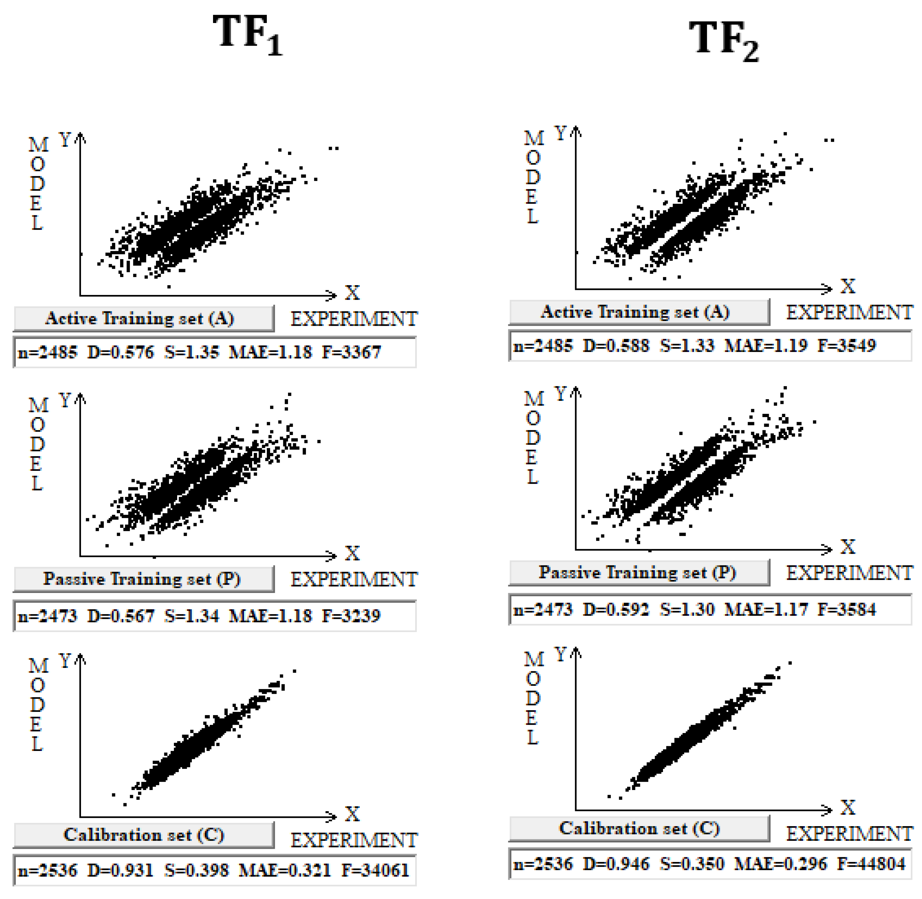
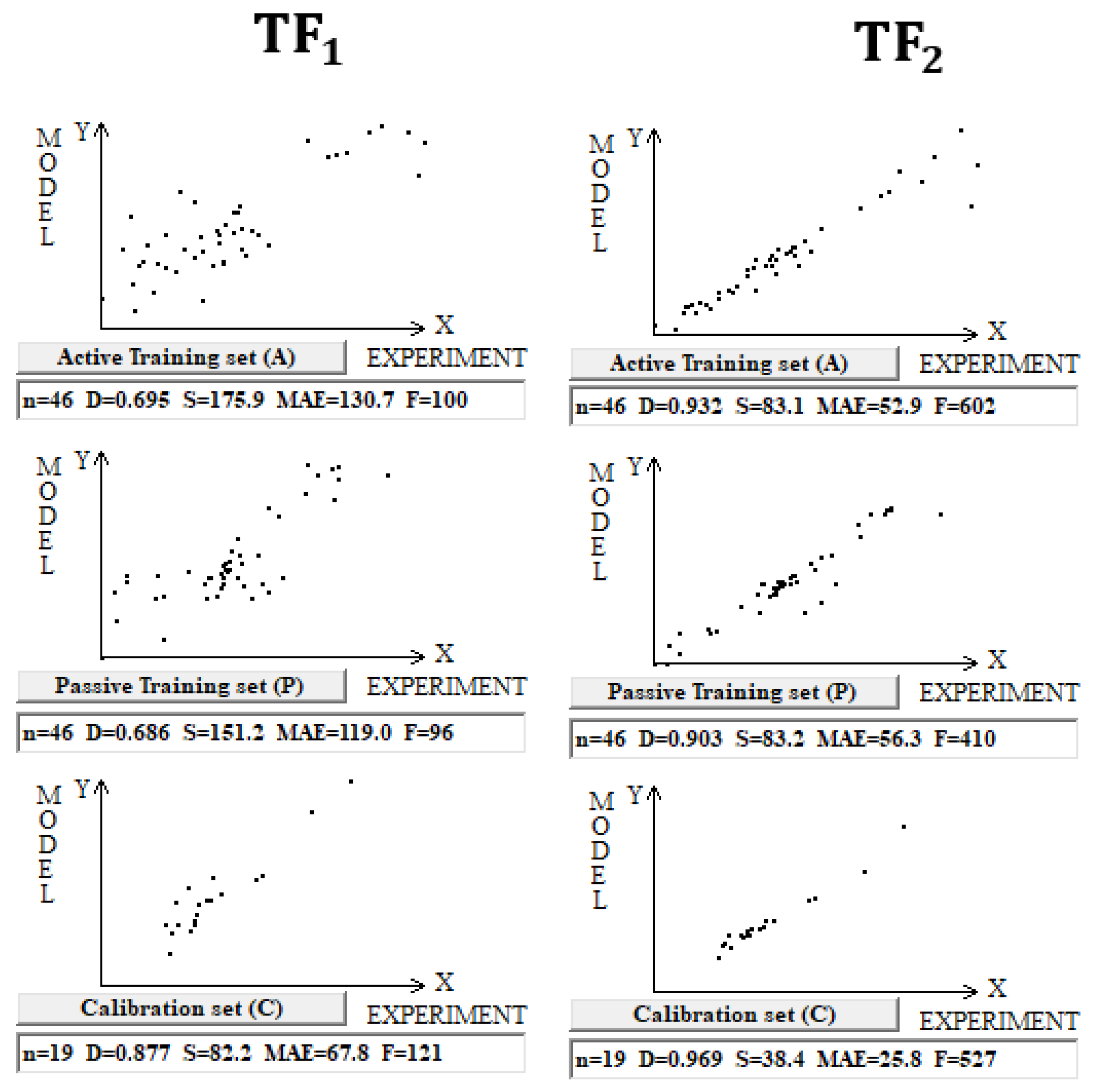
DCW (3,15) was used in this case with 10,005 compounds. Splits into the active training, passive training, calibration, and validation sets were carried out in equal parts. Computer experiments with a full dataset on n-octanol–water partition coefficient, including both organic and inorganic compounds, have shown that the preferred predictive potential is observed if the TF2 is used, i.e., the value of the CCCP is a better indicator of the predictive potential. Figure 1 contains a graphical comparison of these models for the case of models built up using split 1. The data presented in Table 1 for three random splits constructed using the Las Vegas algorithm confirm that TF2 optimization provides the best predictive potential of the models.
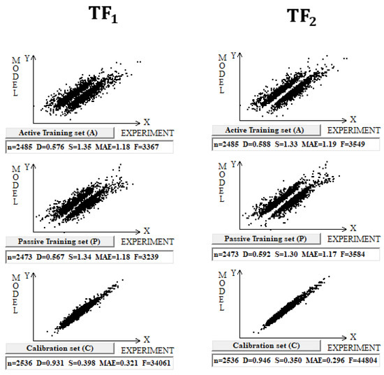
Figure 1.
Comparison of the models calculated with target functions TF1 and TF2 for the set of 10,005 organic and inorganic compounds. Results are shown for the active training set, passive training set, and calibration set for both target functions.

Table 1.
Statistical characteristics of models calculated with Monte Carlo optimization for 10,005 organic and inorganic compounds using target function TF2. The results are provided for three splits. The average determination coefficient on validation sets for TF1 and TF2 models is 0.92 ± 0.01 and 0.94 ± 0.01, respectively.
The division into two correlation clusters for the case of TF1 is due to the use of the IIC [19]. From Figure 1, it is clear that in the case of TF2, where CCCP is applied instead of the IIC, there is also a stratification into correlation clusters, such as that described in [19]. Using the IIC improves the statistical quality of the model for the calibration set, but to the detriment of the training sets [19]. Apparently, the impact of using CCCP in optimizing correlation weights has a similar effect. Poor determination coefficient values for training sets, in fact, are caused by the above clustering into two clusters, which individually have high enough correlation coefficients.
2.2. QSPR Models for Octanol–Water Partition Coefficient Observed for Dataset 2
DCW(3,15) was used in the case of building models for 461 inorganic compounds and small molecules. Splits into the active training, passive training, calibration, and validation sets were carried out in equal parts. Inorganic compounds contain gold, germanium, mercury, lead, selenium, silicon, and tin. In addition, substances with small molecules (in which the number of symbols in the SMILES line is less than 15) are used too. Computational experiments with these compounds have shown that TF2 optimization again gives better predictive potential (Figure 2).
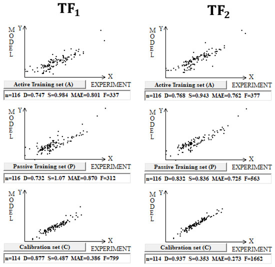
Figure 2.
Comparison of the models calculated with target functions TF1 and TF2 for compounds in dataset 2.
Table 2 contains the completed statistical characteristics of models on three different splits of inorganic compounds. The data presented in Table 2 for three random splits constructed using the Las Vegas algorithm confirm that TF2 optimization provides the best predictive potential of the models.
Table 2.
Statistical characteristics of models calculated with Monte Carlo optimization for 461 inorganic compounds using target function TF2. The average determination coefficient on validation sets for TF1 and TF2 models is 0.85 ± 0.03 and 0.90 ± 0.02, respectively.
2.3. QSPR Models for Octanol–Water Partition Coefficient Observed for Dataset 3 on Pt (IV) Complexes
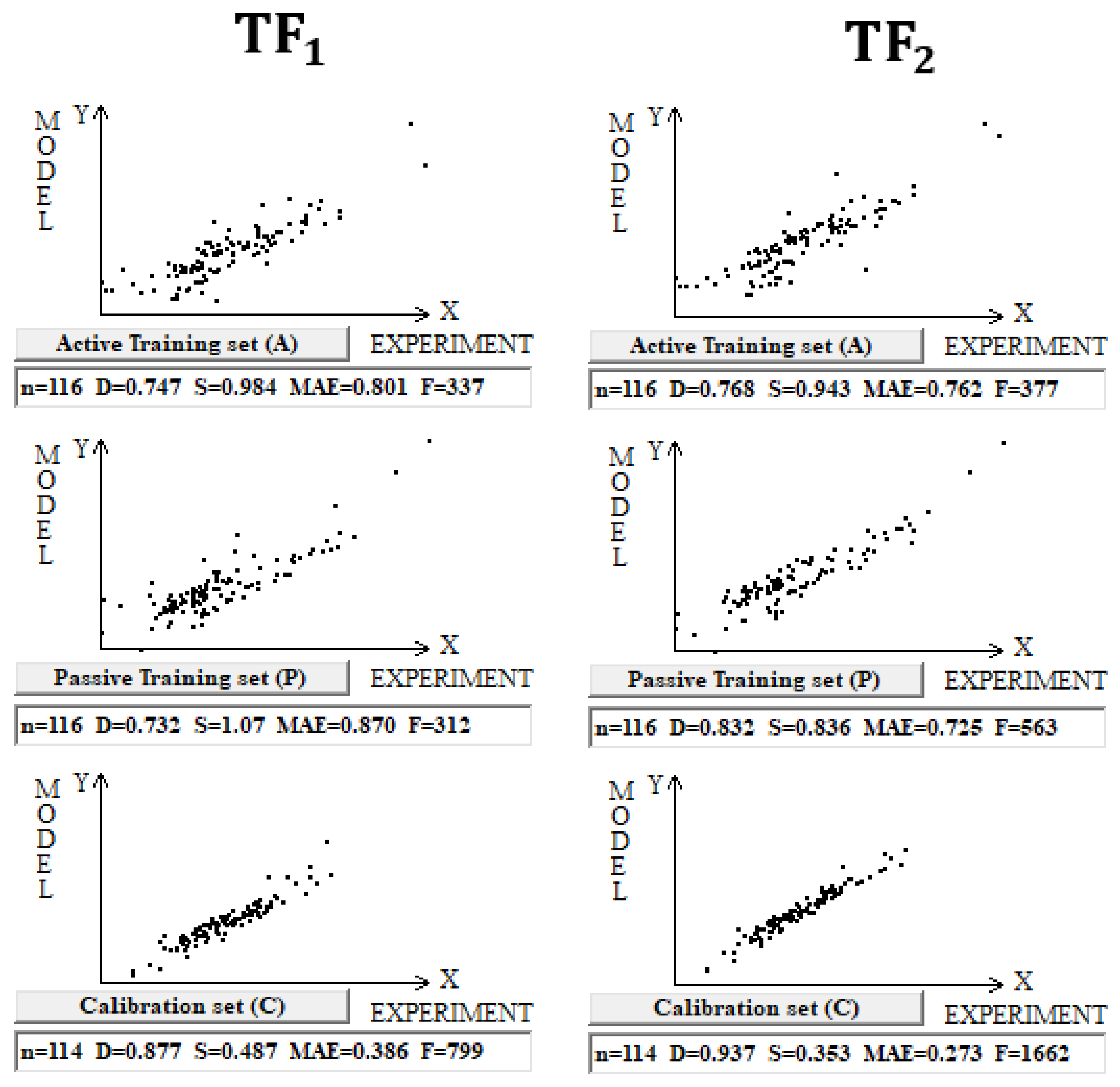
DCW(3,15) was used in the case of building models for 122 Pt (IV) complexes. Splits into the active training, passive training, calibration, and validation sets were carried out in equal parts (Figure 3 and Table 3).
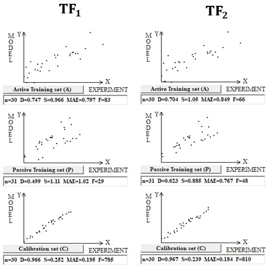
Figure 3.
Comparison of models of logP calculated using target functions TF1 and TF2 for Pt (IV) complexes in dataset 3.
Table 3.
Statistical characteristics of models calculated with Monte Carlo optimization for 122 Pt (IV) complexes using target function TF2. The average determination coefficient on validation sets for TF1 and TF2 models is 0.90 ± 0.03 and 0.94 ± 0.01, respectively.
2.4. QSPR Models for the Enthalpy of Formation for Organometallic Complexes for Dataset 4
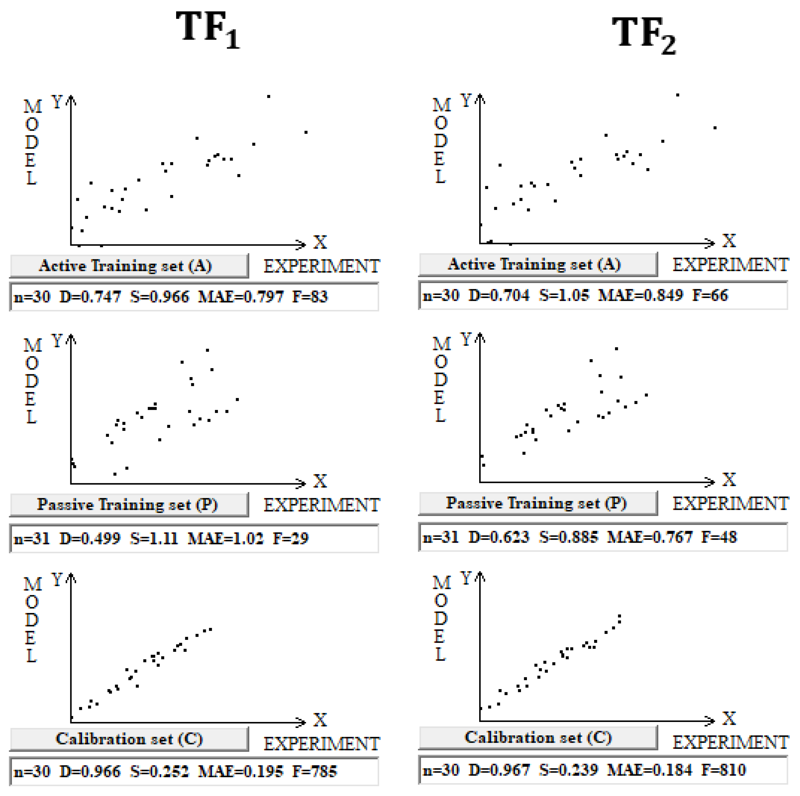
In the case of modeling the enthalpy of formation of organometallic complexes, the active and passive training sets as well as calibration and validation sets were split at 35%, 35%, 15%, and 15%, respectively.
Figure 4 shows again that the preferable predictive potential is observed in the case of TF2 optimization. Table 4 contains the data on the statistical quality of models for the three splits.
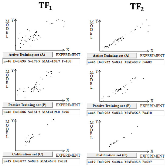
Figure 4.
Comparison of the models of enthalpy of formation for organometallic complexes calculated using target functions TF1 and TF2 (dataset 4).
Table 4.
Statistical characteristics of models for the enthalpy of formation on three splits for the training and validation sets. The average determination coefficient on validation sets for TF1 and TF2 models is 0.93 ± 0.05 and 0.97 ± 0.01, respectively.
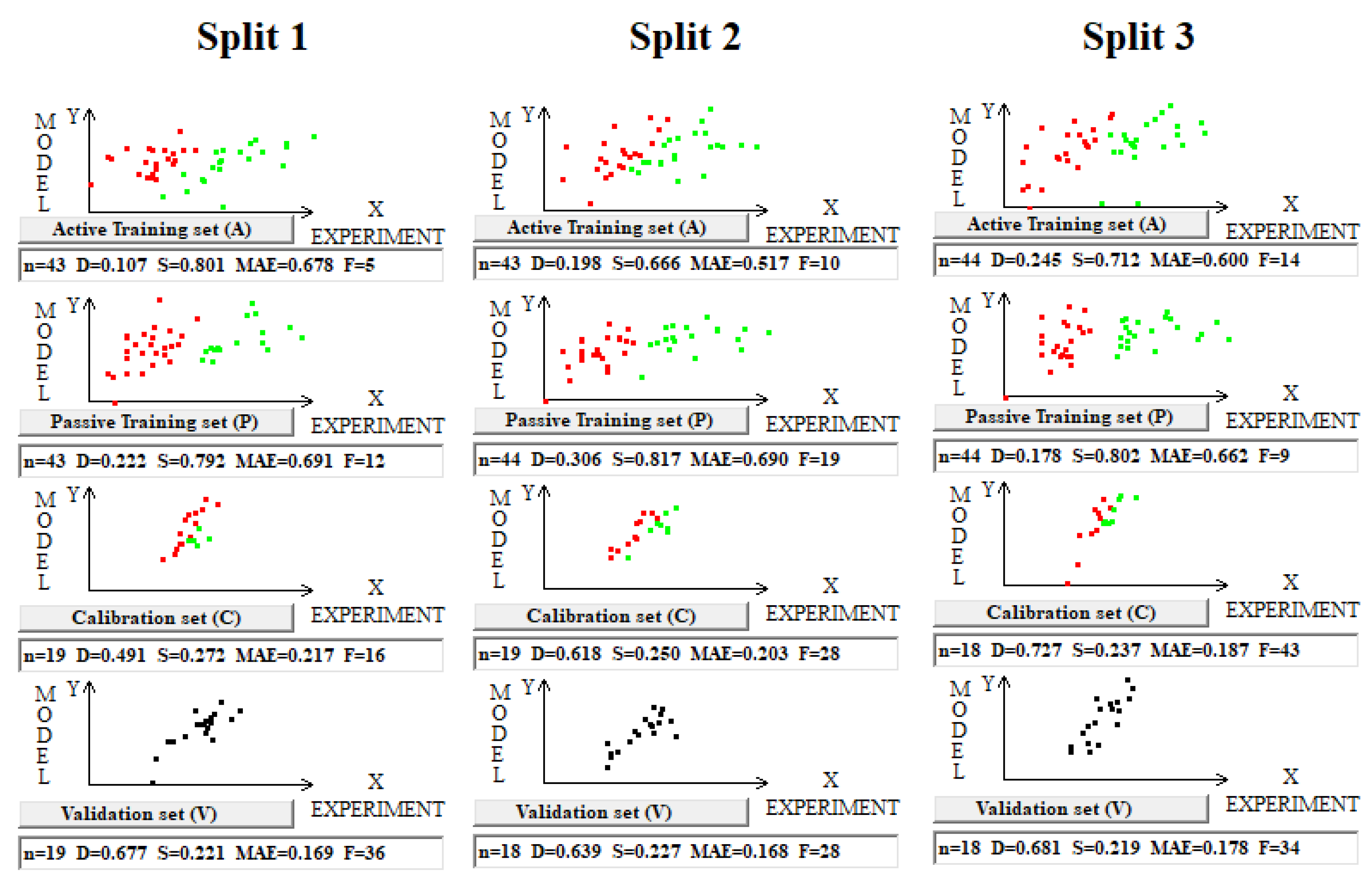
2.5. QSAR Models for Acute Toxicity (pLD50) Toward Rats for Dataset 5
In the case of modeling the toxicity (pLD50) of organometallic complexes, DCW (1,15) was used. The division into active and passive training sets and calibration and validation sets was carried out at 35%, 35%, 15%, and 15%, respectively. Note that the splits are different (Table 5).
Table 5.
Percentages of identity for three splits of dataset 5.
Toxicity modeling according to the scheme applied for the above four described datasets did not yield results (the observed values of the coefficients of determination for the validation sets were close to zero). However, the modeling based on TF1 optimization yielded results with modest statistical parameters (Table 6 and Figure 5).
Table 6.
Statistical characteristics of models for toxicity (pLD50) are evaluated on three splits into the training and validation sets. The average determination coefficient on validation sets for the TF1 models is 0.67 ± 0.02. Attempts to construct models for toxicity using TF2 optimization were unsuccessful.
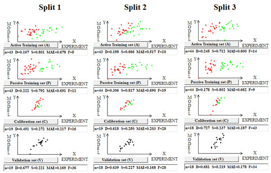
Figure 5.
Graphical representation of models’ toxicity for three splits into the training and validation sets obtained using the Las Vegas algorithm on dataset 5. Red dots indicate where the experimental value minus the calculated value is smaller than zero; otherwise, the dots are green. In the case of the validation set, the clustering is not discussed (all dots are black).
3. Discussion
3.1. IIC and CCCP: Principles and Differences
The IIC is a criterion of the predictive potential of models that combines observed conditions in two directions: (i) from the value of the coefficient of determination; and (ii) from the value of the dispersion of points in the coordinates of the experiment vs. model.
The CCCP criterion is a value developed based on the representation of points that are participants in correlations, similarly to social processes in terms of a “supporter” or “opponent” of the observed correlation. If removing a point results in an increase in the correlation coefficient for the remaining points, then that point is an “opponent” of the correlation. If removing a point results in a decrease in the correlation coefficient for the remaining points, then that point is a “supporter” of the correlation.
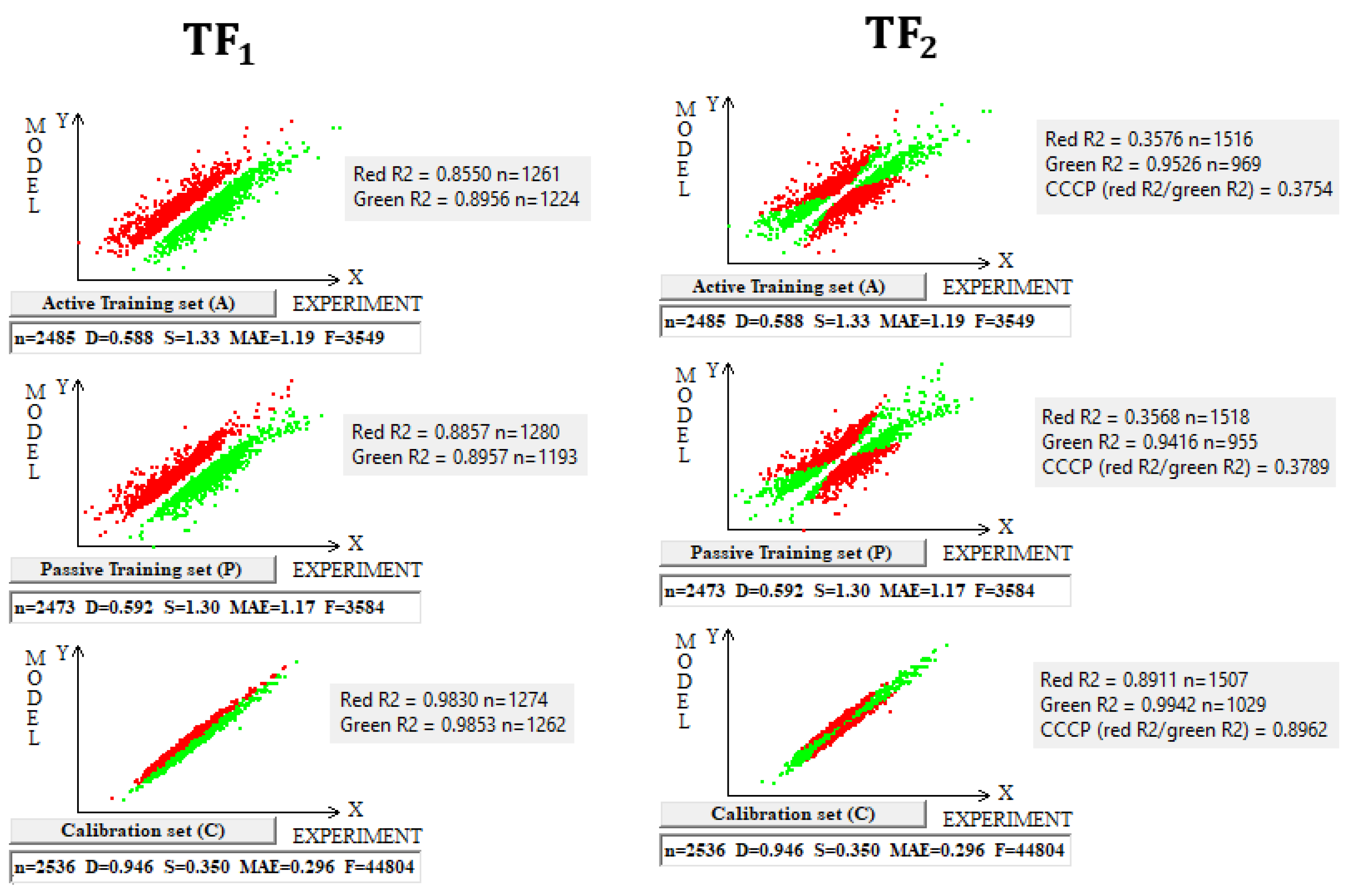
The use of the IIC leads to an improvement in the statistical quality of the model for the calibration set, but to the detriment of the statistical quality of the model for the active and passive training samples. Geometrically, this decrease in the statistical quality on the training samples looks like two parallel clusters (Figure 6). The coefficient of determination calculated for both clusters (red and green) has a value lower than that for each of the mentioned clusters separately. Remarkably, such clusters for the calibration set turn out to be closer to each other than those on the active and passive training sets. There is a probability that these clusters can be close for the validation set too. If so, the model is successful.
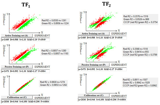
Figure 6.
The geometrical essence of TF1 and TF2 optimizations applied in the study. In the case of TF1, red dots indicate where the experimental value minus the calculated value is smaller than zero; otherwise, the dots are green. In the case of TF2, red dots indicate opponents of correlation, and green dots indicate supporters of correlation.
The use of CCCP aims to obtain completely different correlation clusters to those obtained using the IIC (Figure 6). CCCP aims to obtain close coefficients of determination for the clusters of “supporters” and “opponents” of the correlation. Again, the transformations have the maximum effect on the calibration set, giving the user of the method some hope that this useful effect will be observed in the external calibration set. The different datasets chosen in this study represent quite different properties, related to physicochemical and toxicological endpoints. The interactions of the molecules with the abiotic and biotic external situation are expected to play different roles. Thus, this study may help us explore the possible contributions of specific algorithms to the success of the models. The results of the computer experiments conducted indicate that the CCCP-based approach is effective for large datasets, i.e., for all considered models except for the toxicity of inorganic compounds to rats. Only for the last model was the application of the IIC better than that of CCCP. This may be due to the lower number of substances (a few hundred) in this case.
3.2. Genesis of Models for logP
Conducting a series of runs of the described optimization procedure allowed us to identify collections of molecular features extracted from the SMILES that influence the growth or, conversely, the decrease in the values of the octanol–water distribution coefficients on the datasets considered.
In dataset 1, involving organic and inorganic molecules, the number of promoters of the increase/decrease in logP (Figure 7) is larger than that of promoters of the increase/decrease in the logP of dataset 2 (Figure 8). This is expected; indeed, our models, like most in silico models, have a statistical basis. Thus, if the dataset at the basis of the model is larger, the number of features extracted by the model is very likely larger than the number of features extracted from a smaller dataset. This kind of consideration underlines the relevance of efforts to build up models merging organic and inorganic substances, as we present here. Unfortunately, most in silico models eliminate information on salts due to the technical difficulty of coping with disconnected structures. Furthermore, several models deal only with “classical” atoms present in the organic substances, disregarding organometallic compounds. This aspect is partially due to technical reasons (it is easier to develop certain kinds of models) and partially related to the availability of experimental data for certain compounds (data on certain organometallic substances are more limited than data on classical substances). Thus, even from a technological point of view, it may be feasible to develop models including, for instance, substances like germanium; if the number of substances with germanium is low, we cannot expect to obtain good models based on a large population of substances with very few substances with a specific atom. Nevertheless, it is necessary to address the modeling from a broader perspective, and, in particular, to be aware of the limitations of the current models when dealing with properties where the neutralization of the structure produces a substance with very different properties. This is the case for logP, as studied here.
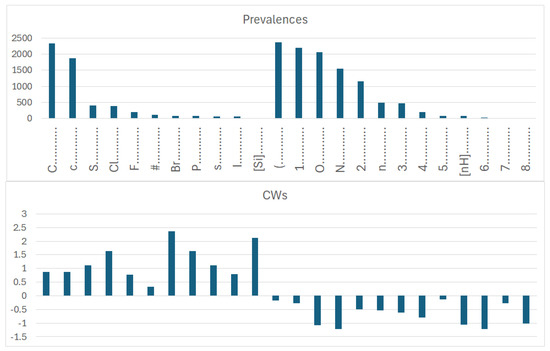
Figure 7.
Prevalence and correlation weights of molecular features extracted from the SMILES, which are promoters of an increase or decrease in logP in the case of dataset 1, which includes both organic and inorganic molecules.
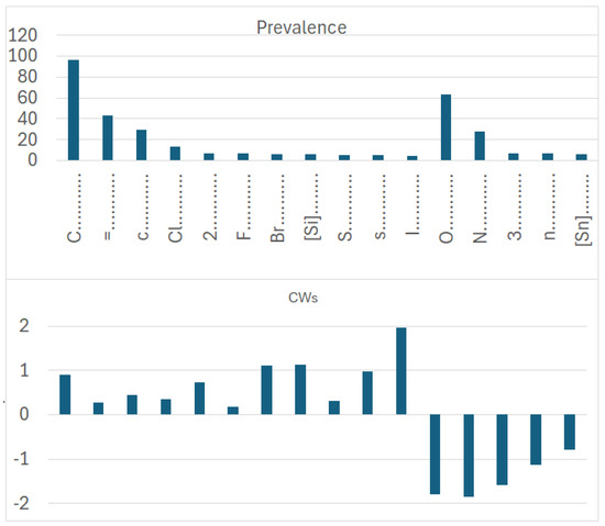
Figure 8.
Prevalence and correlation weights of molecular features extracted from the SMILES, which are promoters of an increase or decrease in logP in the case of dataset 2.
More specifically, for organic substances, the software correctly identifies the role of atoms, such as oxygen and nitrogen, which increase the polarity, and thus decrease logP; conversely, chlorine, bromine, fluorine, and carbon, for instance, increase logP. For inorganic compounds, the main features are present for the organic substances discussed above, but with very different relevance in some cases. In addition, some features are not present at all, such as in the cases with branching and a large number of rings. Obviously, these features are typical of organic substances.
The coefficient serves to clarify the role of SMILES components in increasing or decreasing logP. Figure 9 compares the influence of various correlation weights, indicating that there is some difference in the participation of different features in the organization of the models. Thus, for inorganic compounds, the same features present for organic compounds appear, but sometimes with a different relevance, as represented by the coefficients. This is the case with chlorine, for instance. It appears both in Figure 7 and Figure 8, indicating a role associated with organic and inorganic substances; however, in the case of organic substances, its coefficient is the third largest one, while in the case of inorganic compounds, its coefficient is quite small. This can be explained by the fact that many polychlorinated organic substances largely contribute to the model for logP in the case of organic substances. Bromine and fluorine have a similar behavior, as shown in Figure 9.
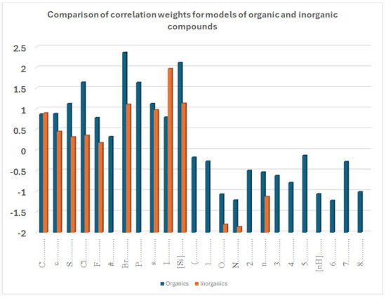
Figure 9.
Comparison of sets of promoters for the increase and decrease in the octanol–water partition coefficient of a model built for datasets 1 and 2.
The list of promoters for the increase and decrease in logP for dataset 3 (Table 7) shows that the property is sensitive to the complexes possessing 3D features, as well as to presence of double bonds. This kind of information is present in dataset 3, which is a quite focused population of substances enabling the investigation of sophisticated features. Thus, one can identify an essential difference between the considered model for organic and inorganic compounds and the model for Pt (IV) complexes. Certain features are common to all datasets. Indeed, oxygen and nitrogen are responsible for an increased polarity, and thus a reduced logP, while branching and chlorine increase logP, as discussed above, for the previous datasets as well.
Table 7.
List of promoters for increasing/decreasing logP for Pt(IV) complexes.
The features relevant for dataset 4 are shown in Table 8. In the case of the models of enthalpy formation, some features increase the enthalpy, with different levels of effect, considering the sign and value of the coefficient. As in the other cases, it is necessary to have consistency between the three runs. Thus, mercury, tin, organic carbon, and a relatively large number of rings (three) increase enthalpy. Conversely, chlorine, boron, branching, and aliphatic carbon decrease the enthalpy. Chlorine is by far the most relevant feature playing a role in enthalpy, followed by boron and mercury.
Table 8.
List of promoters for increasing/decreasing the enthalpy of formation of organometallic complexes.
Table 5 shows the promoters of an increase or decrease in the effect for dataset 5. This dataset concerns acute toxicity in rats. The endpoint is expressed as the negative decimal logarithm of the oral lethal dose. Thus, a higher value is associated with a higher toxicity. The SMILES for the toxicity case, studied with dataset 5, has a different configuration compared to the SMILESs used for the other models because, for these compounds, an important aspect of the structures is the charged particles, which are virtually absent for the other sets of molecules considered here. From Table 9, we can see that nickel has the highest effect. Other salts have a role too. Regarding the organic components of the molecules, aliphatic carbon, double bonds, and branching have a negative coefficient, while the presence of rings has a positive coefficient.
Table 9.
List of promoters for increasing/decreasing the toxicity (pLD50) of organometallic complexes.
Here, as in other datasets, it can be noted that the main differences between the models for organic and inorganic compounds are the sensitivity of organic compounds to branching and the presence of rings. This is quite obvious, since many organic substances are not linear and contain rings. The models correctly identified these peculiar features, and thus, this confirms the correctness of the modeling approach, from a practical point of view and based on the fact that the models are heuristic. The presence of metals, salts, etc., is another feature extracted by the models. This involves the fact that the modeling approach is versatile and can deal with organic and inorganic features simultaneously. Thus, the lack of models for inorganic compounds in the literature is explained only partially by the more limited number of inorganic compounds. A key point in covering the present gap of models on inorganic or combined substances is the use of adequate tools, as demonstrated here.
4. Materials and Methods
4.1. Data
Five datasets were considered in this study. (1) A collection of data on octanol–water partition coefficients was taken from [30]. The dataset contains 10,005 compounds, including organic and inorganic compounds. This is called dataset 1. As a separate exercise, inorganic compounds and substances of small sizes were studied (the number of symbols in the SMILES line was less than 15); this is called dataset 2. Thus, two models were developed for all substances or for only inorganic ones. (2) A collection of data (dataset 3) on octanol–water partition coefficients on platinum (IV) complexes was taken from [31]. (3) A dataset on the enthalpies of formation of organometallic compounds (dataset 4) was taken from [32]. (4) Data on the toxicity of inorganic compounds toward rats (dataset 5), expressed as the negative decimal logarithm of an oral lethal dose for 50% of the tested animals, was taken from [23]. Thus, five models for three endpoints were considered.
For each of the mentioned endpoints, the following actions were performed. First, the available data were divided into training and validation sets. The training set was structured into active and passive training subsets supplemented by a calibration subset. For three of the five models under consideration, the division into an active training set, a passive training set, a calibration set, and a validation set was carried out in equal proportions (i.e., 25% for each of the specified subsets). For datasets 4 and 5, 35% was reserved for the active and passive training sets each, and 15% for the calibration and validation sets each.
4.2. Models
The models for the endpoints under consideration were calculated as
The endpoint was the n-octanol–water partition coefficient or toxicity; DCW(T,N) is an optimal descriptor calculated with the correlation weights of the molecular features extracted from the SMILES [33]. Threshold T is used to define non-rare features, which are involved in the simulation process, and rare features, which are removed from consideration. A molecular feature present in the active training set at least T times is considered non-rare. N is the number of optimization epochs of the correlation weights for non-rare molecular systems calculated using the Monte Carlo method (CORAL software, http://www.insilico.eu/coral, accessed on 27 June 2025).
4.3. Optimimal SMILES Descriptor
The DCW is calculated as
Here, Sk is a SMILES atom, i.e., one symbol (e.g., ‘C’, ‘N’, ‘O’, etc.) or a group of symbols that cannot be considered separately (e.g., ‘Br’, ‘@@’, ‘%11’, etc.) [30]. CW(Sk) is the correlation weight for Sk. In other words, CW(X) is a certain coefficient added to the calculated optimal descriptor every time the SMILES atom is X.
4.4. Optimimization of Correlation Weights
The correlation weights were optimized using the Monte Carlo method. The following are considered target functions of the optimization process:
DA and DP are determination coefficient values for the active and passive training sets, respectively. IIC is the index of ideality of correlation [34], and CCCP is the coefficient of conformism of a correlative prediction [34].
4.5. Applicability Domain
The domain of applicability for the described model is defined via the so-called statistical defects of SMILES codes involved in the optimization process. These defects can be calculated as
where P(Sk), P′(Sk), and P″(Sk) are the probability of Sk in the active training set, passive training set, and calibration set, respectively; and N(Sk), N′(Sk), and N″(Sk) are the frequencies of Sk in the active training set, passive training set, and calibration set, respectively. The statistical defects of SMILES (Dj) are calculated as
where NA is the number of non-rare SMILES atoms.
A SMILES falls in the domain of applicability if
4.6. Mechanistic Interpretation
The correlation weights were optimized several times. In some cases, SMILES atoms exhibited only positive values. The role of these SMILES atoms can be assessed as influencing an increase in the studied endpoint. At the same time, for some SMILES atoms, only negative values of correlation weights were observed. The role of such SMILES atoms can be assessed as influencing a decrease in the studied endpoint. Finally, it is very likely that for some SMILES atoms, alternating sign values of correlation weights are observed. For such SMILES atoms, it is not possible to determine their role in constructing models.
5. Conclusions
In silico models are rapidly evolving and are more and more often applied to evaluate a range of properties for a broad range of substances. However, so far, poor attention has been paid to inorganic substances. A reason for this is the much higher number of organic substances compared to inorganic ones. However, there are also technical reasons, such as it being easier to disregard metal salts when building a model. This causes a bias because in common practice, the substance is neutralized and thus information about the salt is disregarded, while the property of the salt is different from the property of the neutral form. The solubility, logP, etc., of acetic acid or sodium acetate are very different, and these physicochemical properties have an impact on all other properties, such as on their toxicity or environmental behavior. The focus of the studies presented here is to show that it is possible to develop models of both organic and inorganic substances simultaneously and that the models can differentiate the behavior of the substances by extracting features specific to organic or inorganic substances. These models are practical and heuristic. In the computational experiments considered, models for organic compounds are sensitive to branching and the presence of cycles to a much greater extent than those for inorganic compounds. This is quite obvious, but it demonstrates the correctness of the modeling approach. Similarly, for inorganic substances, specific features were identified. The features are different for the different endpoints, but the models can still be used, thus providing good models for all endpoints tested, with the five datasets used. A model should be built for each endpoint several times, obtaining multiple splits into training and validation sets to provide the necessary statistical robustness. Moreover, CCCP is more effective than the IIC as an additional factor in optimizing correlation weights for SMILES-based optimal descriptors when large datasets (hundreds or thousands of data points) are considered. For small datasets (less than a couple of hundred), the IIC may be preferable.
Supplementary Materials
The following supporting information can be downloaded at: https://www.mdpi.com/article/10.3390/inorganics13070226/s1: Table S1. Organic and inorganic compounds, logP; Table S2. Inorganic compounds, logP; Table S3. Pt(IV) complexes, logP; Table S4. Entalpy of formation of organometallic complexes, kJ/mol; Table S5. Toxicity of organometallic and inorganic substances towards rats, pLD50.
Author Contributions
Conceptualization, A.P.T., A.A.T., A.R. and E.B.; methodology, A.P.T., A.A.T., A.R. and E.B.; software, A.A.T.; validation, A.P.T., A.A.T., A.R. and E.B.; formal analysis, A.P.T.; data curation, A.P.T. and A.A.T.; writing—original draft preparation, A.P.T., A.A.T., A.R. and E.B.; writing—review and editing, A.P.T., A.A.T., A.R. and E.B. All authors have read and agreed to the published version of the manuscript.
Funding
We acknowledge EFSA for the financial contribution within project sOFT-ERA, OC/EFSA/IDATA/2022/02.
Institutional Review Board Statement
Not applicable.
Informed Consent Statement
Not applicable.
Data Availability Statement
Data are available in the article and Supplementary Materials, as well on request from the corresponding author.
Conflicts of Interest
The authors declare no conflicts of interest.
References
- Aiello, I.; Aiello, D.; Ghedini, M. Aluminum(III), gallium(III), and indium(III) 4-hydroxyacridinato complexes. J. Coord. Chem. 2009, 62, 3351–3365. [Google Scholar] [CrossRef]
- Pettinari, C.; Tombesi, A. MOFs for electrochemical energy conversion and storage. Inorganics 2023, 11, 65. [Google Scholar] [CrossRef]
- Dai, S.; Yin, Y.; Wang, Y.; Cao, B.; Peruzzini, M.; Barzagli, F. Study on the thermal decomposition kinetics of ammonium carbamate for low-grade heat utilization. Thermochim. Acta 2024, 739, 179809. [Google Scholar] [CrossRef]
- Pettinari, C.; Pettinari, R.; Di Nicola, C.; Tombesi, A.; Scuri, S.; Marchetti, F. Antimicrobial MOFs. Coord. Chem. Rev. 2021, 446, 214121. [Google Scholar] [CrossRef]
- Tombesi, A.; Pettinari, C. Metal organic frameworks as heterogeneous catalysts in olefin epoxidation and carbon dioxide cycloaddition. Inorganics 2021, 9, 81. [Google Scholar] [CrossRef]
- Xhaferaj, N.; Tăbăcaru, A.; Moroni, M.; Senchyk, G.A.; Domasevitch, K.V.; Pettinari, C.; Galli, S. New coordination polymers of zinc(ii), copper(ii) and cadmium(II) with 1,3-Bis(1,2,4-triazol-4-yl)adamantane. Inorganics 2020, 8, 60. [Google Scholar] [CrossRef]
- Haupt, A. Organic and Inorganic Fluorine Chemistry: Methods and Applications; Walter de Gruyter GmbH & Co KG: Berlin, Germany, 2021; pp. 1–626. ISBN 3110659506/9783110659504. [Google Scholar]
- Calabrese, C.; Liotta, L.F.; Soumoy, L.; Aprile, C.; Giacalone, F.; Gruttadauria, M. New hybrid organic-inorganic multifunctional materials based on polydopamine-like chemistry. Asian J. Org. Chem. 2021, 10, 2932–2943. [Google Scholar] [CrossRef]
- Deburgomaster, P.; Zubieta, J. Organic-inorganic hybrid materials: Ligand influences on the structural chemistry of copper-vanadates. Inorg. Chim. Acta 2010, 363, 2912–2919. [Google Scholar] [CrossRef]
- Doctorovich, F.; Di Salvo, F. Performing organic chemistry with inorganic compounds: Electrophilic reactivity of selected nitrosyl complexes. Acc. Chem. Res. 2007, 40, 985–993. [Google Scholar] [CrossRef]
- Gramatica, P. Origin of the OECD Principles for QSAR validation and their role in changing the QSAR paradigm worldwide: An historical overview. J. Chemom. 2025, 39, e70014. [Google Scholar] [CrossRef]
- Natarajan, R.; Natarajan, G.S.; Basak, S.C. Quantitative Structure–Activity Relationship (QSAR) modeling of chiral ccr2 antagonists with a multidimensional space of novel chirality descriptors. Molecules 2025, 30, 307. [Google Scholar] [CrossRef]
- Banerjee, A.; Roy, K.; Gramatica, P. A bibliometric analysis of the Cheminformatics/QSAR literature (2000–2023) for predictive modeling in data science using the SCOPUS database. Mol. Divers. 2024, e3000918. [Google Scholar] [CrossRef]
- Bertato, L.; Chirico, N.; Papa, E. QSAR models for the prediction of dietary biomagnification factor in fish. Toxics 2023, 11, 209. [Google Scholar] [CrossRef] [PubMed]
- Wellnitz, J.; Jain, S.; Hochuli, J.E.; Maxfield, T.; Muratov, E.N.; Tropsha, A.; Zakharov, A.V. One size does not fit all: Revising traditional paradigms for assessing accuracy of QSAR models used for virtual screening. J. Chemom. 2025, 17, 7. [Google Scholar] [CrossRef]
- Halder, A.K.; Cordeiro, M.N.D.S. Applications of predictive QSPR modeling for deep eutectic solvents. In Materials Informatics III. Challenges and Advances in Computational Chemistry and Physics; Roy, K., Banerjee, A., Eds.; Springer: Cham, Switzerland, 2025; Volume 41, pp. 177–203. [Google Scholar] [CrossRef]
- Consonni, V.; Ballabio, D.; Todeschini, R. Chemical space and molecular descriptors for QSAR studies. In Cheminformatics, QSAR and Machine Learning Applications for Novel Drug Development; Roy, K., Ed.; Academic Press: New York, NY, USA, 2023; pp. 303–327. [Google Scholar] [CrossRef]
- Benigni, R.; Bossa, C. Data-based review of QSARs for predicting genotoxicity: The state of the art. Mutagenesis 2019, 34, 25–32. [Google Scholar] [CrossRef]
- Toropov, A.A.; Toropova, A.P.; Roncaglioni, A.; Benfenati, E. The system of self-consistent models for pesticide toxicity to Daphnia magna. Toxicol. Mech. Methods 2023, 33, 578–583. [Google Scholar] [CrossRef] [PubMed]
- Toropova, A.P.; Toropov, A.A.; Fjodorova, N. QSPR and Nano-QSPR: Which one is common? The case of fullerenes solubility. Inorganics 2023, 11, 344. [Google Scholar] [CrossRef]
- Moncho, S.; Serrano-Candelas, E.; de Julián-Ortiz, J.V.; Gozalbes, R. A review on the structural characterization of nanomaterials for nano-QSAR models. Beilstein J. Nanotechnol. 2024, 15, 854–866. [Google Scholar] [CrossRef]
- Trinh, T.X.; Seo, M.; Yoon, T.H.; Kim, J. Developing random forest based QSAR models for predicting the mixture toxicity of TiO2 based nano-mixtures to Daphnia magna. NanoImpact 2022, 25, 100383. [Google Scholar] [CrossRef]
- Toropova, A.P.; Toropov, A.A.; Benfenati, E.; Gini, G. Co-evolutions of correlations for QSAR of toxicity of organometallic and inorganic substances: An unexpected good prediction based on a model that seems untrustworthy. Chemometr. Intell. Lab. Syst. 2011, 105, 215–219. [Google Scholar] [CrossRef]
- Dong, F.; Guo, W.; Liu, J.; Xu, L.; Lee, M.; Song, M.; Li, Z.; Patterson, T.A.; Hong, H. EADB—A database providing curated data for developing QSAR models to facilitate the assessment of endocrine activity. In QSAR in Safety Evaluation and Risk Assessment; Hong, H., Ed.; Academic Press: New York, NY, USA, 2024; pp. 259–272. [Google Scholar] [CrossRef]
- Ferreira, L.T.; Borba, J.V.B.; Moreira-Filho, J.T.; Rimoldi, A.; Andrade, C.H.; Costa, F.T.M. QSAR-based virtual screening of natural products database for identification of potent antimalarial hits. Biomolecules 2021, 11, 459. [Google Scholar] [CrossRef] [PubMed]
- Ghosh, S.; Kar, S.; Leszczynski, J. Ecotoxicity Databases for QSAR Modeling. In Ecotoxicological QSARs. Methods in Pharmacology and Toxicology; Roy, K., Ed.; Humana: New York, NY, USA, 2020; pp. 709–758. [Google Scholar] [CrossRef]
- Burgoon, L.D.; Kluxen, F.M.; Hüser, A.; Frericks, M. The database makes the poison: How the selection of datasets in QSAR models impacts toxicant prediction of higher tier endpoints. Regul. Toxicol. Pharmacol. 2024, 151, 105663. [Google Scholar] [CrossRef] [PubMed]
- Zhu, R.; Tian, S.I.P.; Ren, Z.; Li, J.; Buonassisi, T.; Hippalgaonkar, K. Predicting synthesizability using machine learning on databases of existing inorganic materials. ACS Omega 2023, 8, 8210–8218. [Google Scholar] [CrossRef]
- Wang, X.; He, B.; Liu, B.; Avdeev, M.; Shi, S. A database of electrochemical stability windows containing over 1500 solid-state inorganic compounds. Adv. Funct. Mater. 2024, 34, 2406146. [Google Scholar] [CrossRef]
- Toropov, A.A.; Toropova, A.P.; Cappelli, C.I.; Benfenati, E. CORAL: Model for octanol/water partition coefficient. Fluid Ph. Equilibria 2015, 397, 44–49. [Google Scholar] [CrossRef]
- Toropov, A.A.; Toropova, A.P.; Achary, P.G.R. Prediction of n-octanol–water partition coefficient of platinum (IV) complexes using correlation weights of fragments of local symmetry. Struct. Chem. 2023, 34, 1517–1526. [Google Scholar] [CrossRef]
- Toropova, A.P.; Toropov, A.A.; Benfenati, E.; Gini, G.; Leszczynska, D.; Leszczynski, J. CORAL: QSPRs of enthalpies of formation of organometallic compounds. J. Math. Chem. 2013, 51, 1684–1693. [Google Scholar] [CrossRef]
- Weininger, D. SMILES, a chemical language and information system: 1: Introduction to methodology and encoding rules. J. Chem. Inf. Comput. Sci. 1988, 28, 31–36. [Google Scholar] [CrossRef]
- Toropova, A.P.; Toropov, A.A. The coefficient of conformism of a correlative prediction (CCCP): Building up reliable nano-QSPRs/QSARs for endpoints of nanoparticles in different experimental conditions encoded via quasi-SMILES. Sci. Total Environ. 2024, 927, 172119. [Google Scholar] [CrossRef]


Disclaimer/Publisher’s Note: The statements, opinions and data contained in all publications are solely those of the individual author(s) and contributor(s) and not of MDPI and/or the editor(s). MDPI and/or the editor(s) disclaim responsibility for any injury to people or property resulting from any ideas, methods, instructions or products referred to in the content. |
© 2025 by the authors. Licensee MDPI, Basel, Switzerland. This article is an open access article distributed under the terms and conditions of the Creative Commons Attribution (CC BY) license (https://creativecommons.org/licenses/by/4.0/).