Research of Phase Compensation Methods Based on the Median Reweighted Wirtinger Flow Algorithm

Abstract

An improved non-convex optimized phase recovery algorithm is used to compensate for wavefront aberrations caused by atmospheric turbulence and pointing errors in the vortex beam. The algorithm is divided into two parts: initialization and iteration. To reduce the effect of outliers, truncation rules are formulated in the initialization phase using the robustness of the sample median to obtain an initial value that is close to the global optimum. The relationship between the results of adjacent iterations is used in the iterations to calculate new weight coefficients, which are applied to the gradient descent to ensure the accuracy of the recovery results. Simulation experiments are carried out for different channel environments and different modes, and the results show that the improved phase recovery algorithm can accurately compensate for distorted wave fronts. The improved algorithm recovers the best results at different turbulence intensities and under the influence of different pointing errors. The recovered Strehl ratio can reach 0.9 and the mode purity can reach 0.92. Single-mode and multi-mode simulations were carried out, and the results show that the improved algorithm is effective and robust.

1. Introduction

The understanding of optical vortices has reached new heights due to the further expansion of the research areas involved in this field. Researchers have discovered the orbital angular momentum (OAM) [1] property of photons, which can be used to greatly increase the channel capacity and spectral efficiency of optical communications. Vortex beams also have important potential applications in areas such as radio frequency and quantum-secure communications due to their topological charge. As a result, the development of orbital angular momentum free space optical [2] communication (OAM-FSO) system performance can achieve a wireless communication method with high information capacity, high spectral efficiency and high transmission confidentiality. Orbital angular momentum free-space optical communication systems refer to communication systems that use a vortex beam as a transmission beam. OAM has a theoretically infinite number of mode combinations, allowing for further increases in channel capacity as well as spectral efficiency. When the vortex beam is transmitted in free space, it is inevitably affected by atmospheric turbulence and pointing errors (PE), which distort its spiral phase and lead to inter-mode crosstalk and degraded communication performance [3]. Therefore, eliminating the interference caused by atmospheric turbulence and pointing errors on the phase is one of the main objectives of FSO communication systems.

In recent years, adaptive optics (AO) techniques [4] have been introduced into OAM-FSO communication systems as a class of effective compensation methods for the suppression of turbulent interference, with good results. Depending on whether a wavefront sensor (WFS) is used or not, systems are classified as WFS-based AO systems or WFSless-AO systems [5]. The WFS-AO system has been widely used in the fields of astronomical observation, biomedicine and optical imaging, but its applications are limited by the complexity of the system structure [6]. The WFSless-AO system evaluates the quality of the detected light intensity information and finds the control signal that makes the evaluation result reach the extreme value by means of an optimization-seeking algorithm, which has the advantages of simple structure, small size and low cost [7]. One of the commonly used methods for WFSless-AO systems is the phase recovery algorithm, of which the Gerchberg–Saxton (GS) algorithm is an indirect measurement method for reconstructing the wavefront phase from the wavefront intensity. In the literature [8], Gaussian probe light and the GS algorithm are used to achieve turbulence compensation for carrying OAM beams, and experimental results show that the purity of the pre-compensated beams is improved. In order to reduce the burden on the system, the authors of [9] propose that the detection beam is not required and only the GS algorithm is used to compensate for wavefront aberrations, with good results. In [10], the communication uses a GS algorithm without a beacon beam to compensate for the distorted spiral phase, increasing the mode purity to 0.92. The authors of [11] propose an improved GS algorithm which can significantly compensate for beam aberrations in single-channel or OAM-multiplexed systems. The above study shows the effectiveness of the GS algorithm, but its real-time performance is poor. The study by the authors of [12] compares the correction performance of a GS-based algorithm and a hybrid input–output (HIO) algorithm under a marine turbulent channel, and the results show that the HIO-based compensation performance is better and converges faster. In [13], a GS-HIO-hybrid-algorithm-assisted AO system was proposed to mitigate turbulence effects in random amplitude mask-based underwater wireless optical communication systems, and high accuracy was achieved with only amplitude measurements obtained. A polarization-detection-beam-assisted AO system is proposed in [14] to overcome the effects of atmospheric turbulence through a single-intensity measurement phase retrieval algorithm, effectively improving the mode purity of the OAM beam in different states. Recently, the non-convex optimization algorithm Wirtinger Flow (WF) [15] was shown to converge stably to a globally optimal solution, and unlike the traditional GS HIO algorithm, The WF algorithm has the advantage of not requiring a priori information about the signal. The WF algorithm iterates in signal space, alleviating the need for computation and storage, and a number of variants of the algorithm have been developed. A truncated WF (Truncated Wirtinger Flow, TWF) algorithm was proposed in [16], which successfully eliminates the influence of gradients with low reliability on the recovery results and shortens the convergence times. The gradient components are weighted in [17] using reweighting to ensure that information at any scale can be recovered within a reasonable amount of computation. The authors of [18] propose the conjugate gradient WF algorithm, which significantly increases the convergence rate. The authors of [19] introduce the WF algorithm in wavefront distortion compensation, and experiments show that the WF algorithm is more efficient than the GS algorithm and effectively eliminates the effect of atmospheric turbulence. The authors of [20] combine the WF algorithm and deep learning to outperform the traditional WF algorithm in terms of reconstruction results at low sample complexity. The authors of [21] use the generalized WF algorithm for accurate imaging of the target and achieve accurate image recovery through super-resolution. The above research shows that different iterative algorithms achieve good results in phase recovery, but the WF and its variants have less computation time and higher accuracy. Since the WF algorithm requires an appropriate choice of initial estimates, its performance in complex environments is worth investigating.

To address this, this paper develops new initialization and gradient descent rules based on the original WF algorithm to reduce the computational complexity while ensuring the accuracy of the results, naming it the Median Reweighted WF (MRWF) algorithm. The MRWF algorithm obtains the global optimum in an iterative calculation, and in the same way as the initial WF algorithm this algorithm also runs in two stages. The first stage is the initialization stage, where truncation rules are set based on the sample median, and the stability of the sample median is used to eliminate the effects of outliers, so that the initial estimate is sufficiently close to the global optimum. The second stage is the gradient refinement stage, which uses a reweighting-based gradient descent algorithm to calculate the weights using the ratio of the results of adjacent iterations, ensuring that the direction of the iterations is always close to the true value. Experimental simulations for different channel conditions and different modes show that the MRWF algorithm recovers the best results and that multiple modes do not affect the recovery results of the algorithm.

2. OAM-FSO Model Based on Phase Recovery Algorithm

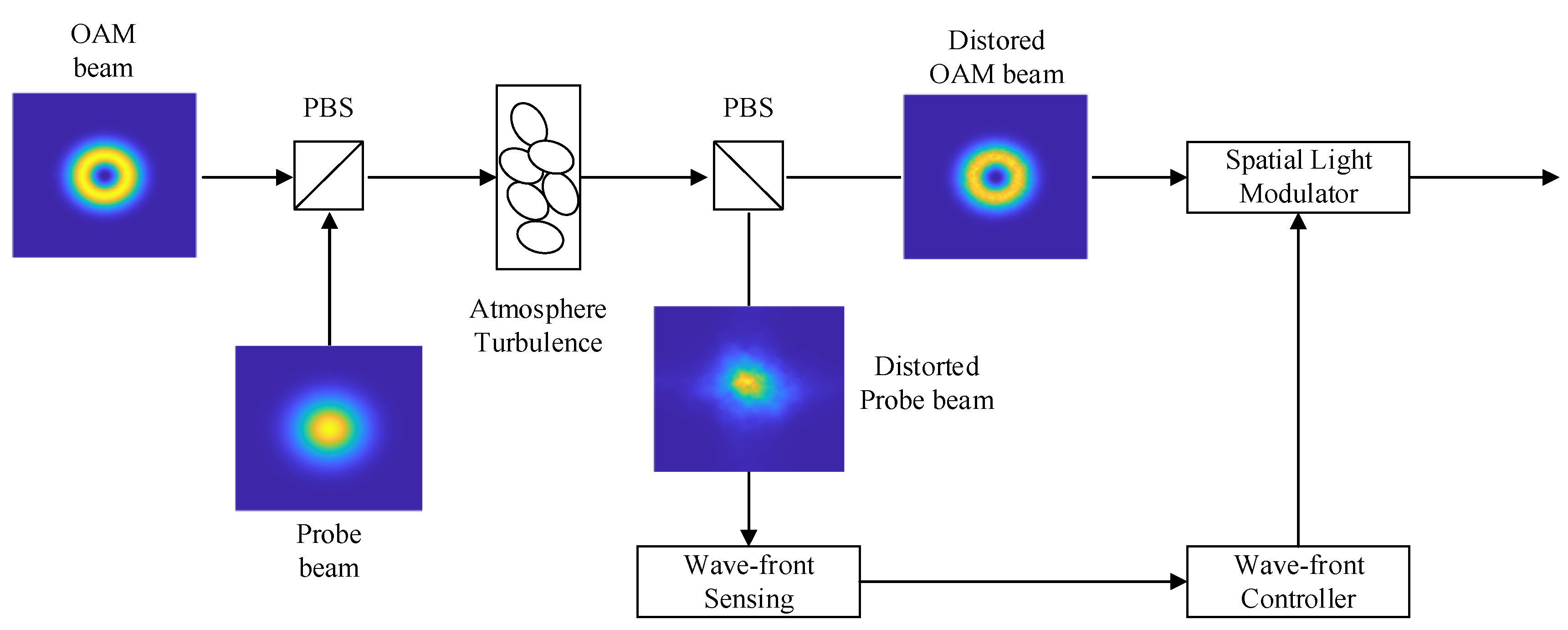
At the transmitting end, the OAM beam carrying the information and the probe beam are combined by a polarized beam splitter (PBS) and transmitted coaxially. The phase distortion caused by atmospheric turbulence is therefore similar throughout the transmission process. At the receiving end, the aberration multiplexed beam is separated by the PBS into an OAM beam as well as a probe beam. The probe beam is then fed into the AO system and the phase distortion caused by atmospheric turbulence during transmission is calculated. Since the phase of the probe light at the transmitter is zero, the phase calculated at the receiver is its distorted phase. Finally, a phase opposite to the aberration is superimposed on the OAM beam split by the spatial light modulator to eliminate the wavefront aberration of the OAM beam. The AO-based OAM-FSO system is shown in Figure 1.

In the OAM-FSO communication system, a Laguerre Gaussian (LG) beam is used as the transmission beam and the LG beam has an expression for its optical field [1] in free space as shown in the following equation.

$$\begin{array}{ll}{u}_p^l(r,\phi ,z)=& \sqrt{\frac{2p!}{\pi (p+\left|l\right|)!}}\frac{1}{w(z)}{\left[\frac{\sqrt{2}}{w(z)}\right]}^{\left|l\right|}\times \\ & L_p^{\left|l\right|}\left[\frac{2r^2}{w^2(z)}\right]\exp \left[\frac{-r^2}{w^2(z)}\right]\times \\ & \exp (-il\phi )\exp \left[\frac{ik{r}^{2}z}{2(z^2+z_0^2)}\right]\times \\ & \exp \left[-i(2p+\left|l\right|+1)\arctan \left(\frac{z}{z_0}\right)\right]\end{array}$$

(1)

where $p$ is the radial index of the LG beam; $l$ is the topological charge of the vortex beam, which can be taken as any integer; $L_p^{\left|l\right|}$ is the Laguerre polynomial; $r$ is the radial distance from the spatial point to the transmission axis; $\phi$ is the azimuth; $k=2\pi /\mathsf{\lambda }$ is the wave number; $\mathsf{\lambda }$ is the wavelength; $w(z)=w_0\sqrt{1+{(z/z_0)}^2}$, $w_0$ is the beam waist radius; $z_0=\pi w_0/\mathsf{\lambda }$ is the Rayleigh distance.

In the simulation of beam transmission, the distribution propagation method is used and the phase screens are arranged sequentially during transmission. When the transmission distance is $\Delta z$, the expression for the light field [6] is shown in the following equation.

$$u(r,\phi ,z_{i+1})={ℱ}^{-1}\left\{ℱ\left\{u(r,\phi ,z_i)\exp \left[i\varphi \left(r,z_i\right)\right]\right\}\exp \left[\frac{-i\left(k_x^2+k_y^2\right)\Delta z}{2k}\right]\right\}$$

(2)

where ${ℱ}^{-1}$ and $ℱ$ denote the Fourier inverse transform and Fourier transform, respectively; $\varphi (r,z_i)$ denotes the atmospheric turbulence phase screen function; $k_x$ and $k_y$ denote the number of spatial waves in the $x$ and $y$ directions, respectively; and $k=\sqrt{k_x^2+k_y^2+k_z^2}$. Next, the Zernike polynomial defined by Noll [7] is chosen to model the turbulence phase screen $\varphi (r)$, which can be expressed by the following equation.

$$\varphi (r)={\displaystyle \sum _i{a}_i{Z}_i}$$

(3)

$$\{\begin{array}{c}{Z}_{eveni}=\sqrt{n+1}{R}_n^m\left(r\right)\sqrt{2}\cos \left(m\theta \right),m\ne 0\\ Z_{oddi}=\sqrt{n+1}{R}_n^m\left(r\right)\sqrt{2}\sin \left(m\theta \right),m\ne 0\\ Z_i=\sqrt{n+1}{R}_n^0\left(r\right),m=0\end{array}$$

(4)

$$R_n^m\left(r\right)={\displaystyle \sum _{s=0}^{\left(n-m\right)/2}{\left(-1\right)}^s\frac{\left(n-s\right)!}{s!\left[\left(n+m\right)/2-s\right]!\left[\left(n-m\right)/2-s\right]!}{r}^{n-2s}}$$

(5)

where $r$ and $\theta$ are polar coordinates; $Z_i$ is an ith order zernike polynomial; $n$ and $m$ are radial and angular orders, respectively, always integer and satisfying the following condition: $m\le n,n-\left|m\right|=even$. The first term of the Zernike polynomial represents the translation and has no effect on the image quality, so the first term is ignored and a polynomial of order 66 is chosen to generate a realistic phase screen of atmospheric turbulence. For Kolmogorov turbulence theory, the covariance between polynomials should satisfy the following equation.

$$E\left(Z_i,Z_j\right)=\frac{K_{zz{}^{\prime }}{\delta }_{mm{}^{\prime }}\mathrm{\Gamma }\left[\left(n+n{}^{\prime }-5/3\right)/2\right]{\left(D/r_0\right)}^{5/3}}{\mathrm{\Gamma }\left[\left(n-n{}^{\prime }+17/3\right)/2\right]\mathrm{\Gamma }\left[\left(n{}^{\prime }-n+17/3\right)/2\right]\mathrm{\Gamma }\left[\left(n+n{}^{\prime }+23/3\right)/2\right]}$$

(6)

$$K_{zz{}^{\prime }}=2.2698{\left(-1\right)}^{\left(n+n{}^{\prime }-2m\right)/2}\sqrt{\left(n+1\right)\left(n{}^{\prime }+1\right)}$$

(7)

where ${\delta }_{mm{}^{\prime }}$ is the Kronecker function and $\mathrm{\Gamma }$ is the gamma function. Based on the above equation, the coefficients in front of the Zernike polynomial can be determined to simulate a phase screen of atmospheric turbulence consistent with Kolmogorov’s turbulence theory, and thus investigate the effect of atmospheric turbulence on light field transport.

In free-space optical communication, the pointing error effect caused by atmospheric turbulence in the beam, as well as jitter in the transmitter and receiver, is also an important factor in good or bad communication performance. Pointing errors, which cause the beam to expand and shift as it reaches the receiver, can be classified as either lateral offset or angular offset errors. The expression for a beam affected by pointing errors is shown in the following equation.

$$U_{pe}(r,\phi ,z)=u\left(r(\cos \phi -\cos \rho ),r(\sin \phi -\sin \rho ),z\right)\exp (ik\tan \alpha \cdot r\sin \phi )$$

(8)

where $\rho$ is the degree of lateral offset and $\alpha$ is the degree of angular offset. $d$ is used in this paper to represent the magnitude of the lateral offset. To evaluate the performance of the algorithm, commonly used performance metrics are chosen as benchmarks. The Strehl ratio (SR) [22] of a beam can effectively characterize the degree of beam front aberration and is a commonly used performance evaluation function, which is the ratio of the central light intensity of the received beam to the central light intensity of the ideal beam. The modal purity of the orbital angular momentum [14] can be expressed as the ratio of the power retained by the aberrated beam at the original emission order to the total power, with a larger value for the current mode indicating a better recovery. The specific equation is shown in the following.

$$SR=\frac{\max [I(x,y)]}{\max [I_0(x,y)]}$$

(9)

$$P_l=\frac{{\displaystyle {\int }_0^{\infty }{\left|a_l(r,z)\right|}^{2}rdr}}{{\displaystyle \sum {\displaystyle {\int }_0^{\infty }{\left|a_m(r,z)\right|}^{2}rdr}}}$$

(10)

$$a_l(r,z)=\frac{1}{\sqrt{2\pi }}{\displaystyle {\int }_0^{2\pi }u(r,\phi ,z)}\exp (il\phi )d\phi$$

(11)

where $I$ is the actual light intensity factor, $I_0$ is the ideal light intensity factor and $P_l$ is the ratio of the individual mode power to the total power.

3. Phase Correction Based on MRWF Algorithm

When communicating in a severe channel environment, where there are anomalous noise values during transmission, the performance of general GS algorithms is challenged and it is extremely easy to get stuck in the wrong direction during iterations. In practice, due to factors such as detector faults and poor channel conditions, the measured values collected often change abruptly and the anomalies are so large that the phase information cannot be recovered properly. In this case, the WF algorithm based on non-convex optimization can achieve better results, but there is still the problem of long computation time, and accuracy needs to be improved. Therefore, this paper uses a median truncation operation to reduce the computational complexity in the initialization stage and uses a reweighted gradient descent method to ensure the accuracy of the recovery results. The mathematical description of a noise-laden phase retrieval problem is expressed as shown in the following equation.

$$y={\left|\langle a_i,x\rangle \right|}^2+\eta$$

(12)

where $\langle \cdot \rangle$ denotes the inner product, $y={[y_1,...,y_m]}^T$ is the measured signal strength information, $A={[a_1,...,a_m]}^T$ is the measurement matrix, $\eta$ is the noise vector, and phase retrieval means recovering the original signal $x$ from the measurement information. Based on the intensity-based least squares empirical loss function proposed in [15], the phase recovery problem can be formulated as the following equation.

$$\min f(z):=\frac{1}{2m}{\displaystyle \sum _{i=1}^m{\left(y_i-{\left|a_i^{H}z\right|}^2\right)}^2}$$

(13)

Due to the modulus, Equation (13) is a non-convex function and requires an optimization algorithm for phase recovery. The authors of [23] express the relationship between the measured and true values in terms of the square of the normalized inner product, expressed in Equation (14) as:

$${\cos }^2{\theta }_i=\frac{{\left|a_i,x\right|}^2}{{\Vert a_i\Vert }^2{\Vert x\Vert }^2},i=1,2,\dots ,m$$

(14)

where $\theta$ is the angle between and $a_i\sim \mathcal{N}(0,I_n)\in {ℝ}^n/{ℂ}^n$ and $x\in {ℝ}^n/{ℂ}^n$; $\theta$ denotes the relationship between the two. It is noted in [23] that in higher dimensional spaces, ${\cos }^2{\theta }_i$ tends to zero, and $a_i$ and $x$ are almost always orthogonal. Therefore, the cosine squared between two vectors should be as small as possible. Based on this property, $\left\{{\cos }^2{\theta }_i\right\}$ is sorted and the smallest value is selected. As can be seen from Equation (14), the size of $\Vert x\Vert$ does not affect the sorting, so for ease of calculation, set $\Vert x\Vert =1$.

To obtain the optimal initial estimate, the following objective function is defined.

$${\displaystyle \sum _{i\in {ℐ}_0}{\cos }^2{\theta }_i}={\displaystyle \sum _{i\in {ℐ}_0}\frac{{\left|a_i,x\right|}^2}{{\Vert a_i\Vert }^2{\Vert x\Vert }^2}}=\frac{x^T}{\Vert x\Vert }\left({\displaystyle \sum _{i\in {ℐ}_0}\frac{a_i{a}_i{}^T}{{\Vert a_i\Vert }^2}}\right)\frac{x}{\Vert x\Vert }$$

(15)

${ℐ}_0$ is the index of the set of cosine squares, and the approximation is obtained by replacing $x$ with the optimizing variable $z$, giving Equation (16).

$$\widehat{z}=\underset{\Vert z\Vert =1}{\min }{z}^{T}Yz$$

(16)

where

$$Y:=\frac{1}{\left|{ℐ}_0\right|}{\displaystyle \sum _{i\in \left|{ℐ}_0\right|}\frac{a_i{a}_i{}^T}{{\Vert a_i\Vert }^2}}$$

(17)

$Y$ is a semi-positive definite matrix and Equation (16) is the minimum eigenvalue of $Y$. When the signal dimension is large, matrix decomposition and inversion becomes very complicated. According to the Strong Law of Large Numbers (SLLN), the sample covariance matrix [23] can be simplified as shown in the following equation.

$$\frac{1}{m}{\displaystyle \sum _{i\in 1}^m\frac{a_i{a}_i{}^T}{{\Vert a_i\Vert }^2}}\approx \mathbb{E}\left[\frac{a_i{a}_i{}^T}{{\Vert a_i\Vert }^2}\right]=\frac{I_n}{n}$$

(18)

$${\displaystyle \sum _{i\in \left|{ℐ}_0\right|}\frac{a_i{a}_i{}^T}{{\Vert a_i\Vert }^2}}={\displaystyle \sum _{i\in 1}^m\frac{a_i{a}_i{}^T}{{\Vert a_i\Vert }^2}}-{\displaystyle \sum _{i\in \left|\overline{{ℐ}_0}\right|}\frac{a_i{a}_i{}^T}{{\Vert a_i\Vert }^2}}\approx \frac{m{I}_n}{n}-{\displaystyle \sum _{i\in \left|\overline{{ℐ}_0}\right|}\frac{a_i{a}_i{}^T}{{\Vert a_i\Vert }^2}}$$

(19)

where $\overline{{ℐ}_0}$ is the complementary set of ${ℐ}_0$. We can rewrite Equation (16) as the following equation.

$$\tilde{z}=\arg \underset{\Vert z\Vert =1}{\max }{z}^T\overline{Y}z$$

(20)

The final problem is therefore simplified to Equation (21).

$$\overline{Y}=\frac{1}{\left|\overline{{ℐ}_0}\right|}{\displaystyle \sum _{i\in \left|\overline{{ℐ}_0}\right|}\frac{a_i{a}_i{}^T}{{\Vert a_i\Vert }^2}}$$

(21)

The initial value can be obtained by solving for the eigenvector corresponding to the largest eigenvalue of Equation (21), which simplifies the computational effort by simple power iterations. To increase the robustness of the algorithm to outliers, the TWF algorithm is initialized with a truncated spectrum method, which avoids the effect of too-large outliers on the results by means of truncation rules. On this basis, the median truncation [24] operation is chosen in this paper to avoid the effects of outliers, and the initial estimate of the median truncation can be expressed by Equation (22).

$$z_0={\mathsf{\lambda }}_0\tilde{z}$$

(22)

where ${\mathsf{\lambda }}_0=\sqrt{med(y)/0.455}$, $med(\cdot )$ indicates a median operation. The median truncation initialization can eliminate the impact of too large or too small outliers. Usually, outliers have a greater impact on the sample mean, whereas the median information is more stable and less susceptible to extremely small values, so using the sample median in the truncation rule can effectively remove the impact of outliers.

After obtaining a more desirable initial estimate, it needs to be updated iteratively to reconstruct the signal. The Wirtinger gradient of Equation (13) is shown in the following equation.

$$\nabla f(z)=\frac{1}{m}{\displaystyle \sum _{i=1}^m\left(y_i-{\left|a_i{}^{H}z\right|}^2\right)\left(a_i{a}_i{}^H\right)}z$$

(23)

The gradient refinement phase of the WF algorithm is solved by a similar gradient descent approach to that used in Equation (13). The full gradient descent algorithm is computationally intensive and tends to fall into a local optimum solution. This paper therefore uses a random average gradient approach to overcome this problem. The iterative formula can be represented by Equation (24).

$$z_{k+1}=z_k-{\mu }_k\frac{1}{m}{\displaystyle \sum _{i=1}^m\nabla f_i(z_k)}$$

(24)

where $k$ is the number of iterative steps and $\mu$ is the step length. Generally, fixed step lengths tend to trap the solution in a local optimum, so the step length is varied by a heuristic [15], represented by Equation (25).

$${\mu }_k=\min \left(1-e^{-k/k_0},{\mu }_{\max }\right)$$

(25)

Experiments have shown that the best results are achieved when and $k_0\approx 330$ and ${\mu }_{\max }\approx 0.4$.

Without considering the time cost, the WF algorithm can converge steadily to the maximum likelihood estimate in the presence of Gaussian noise. In contrast, time is the most important point to consider in practical phase recovery tasks. Therefore, this paper further reduces the computational effort of the algorithm by adding a new truncation rule to the gradient descent process. To ensure that the iterative update values move in the direction of the true value, different weights $w$ are added to each iteration so that they find the correct direction in the iteration. The gradient algorithm with weights is expressed as Equation (26) (see Algorithm 1).

$$z_{k+1}=z_k-{\mu }_k\frac{1}{m}{\displaystyle \sum _{i=1}^m{w}_i^k\nabla f_i(z_k)}$$

(26)

where

$$w_i^k=\{\begin{array}{l}\frac{{\epsilon }_i}{\left|{\left|\langle a_i,z_k\rangle \right|}^2-y_i\right|+{\epsilon }_i} i,k=1\\ \frac{\left|{\left|\langle a_{i-1},z_{k-1}\rangle \right|}^2-y_{i-1}\right|}{\left|{\left|\langle a_i,z_k\rangle \right|}^2-y_i\right|+{\epsilon }_i} i,k>1\end{array}$$

(27)

${\epsilon }_i$ is a parameter that prevents the denominator from going to zero and is set as a fixed parameter in this paper (see Algorithm 1). A weight is added to the gradient component by calculating the ratio of neighboring iterations, the purpose of this weight being to keep the direction of the iterations close to the true value. Adding weight parameters to all gradient components in each iteration of the calculation increases the importance of good gradient components and also preserves the information carried by relatively unreliable gradient components.

The implementation of the median reweighted WF algorithm used in this paper is summarized as follows.

Algorithm 1: Median Reweighted WF algorithm (MRWF)

$\mathbf{Input}:\mathrm{Measurement}\mathrm{intensity}y={\left|\langle a_i,x\rangle \right|}^2+\eta \langle \cdot \rangle$$;\mathrm{step}\mathrm{factor}{k}_0=330$$,{\mu }_{\max }=0.4;$

$\mathrm{weight}\mathrm{factor}{\epsilon }_i=0.1$; maximum number of iterations $K$.

$\mathbf{Initialize}: \mathrm{Set} z_0={\mathsf{\lambda }}_0\tilde{z}$$, \mathrm{where} {\mathsf{\lambda }}_0=\sqrt{med(y)/0.455},$$\widetilde{ z} \mathrm{is}$

$\overline{Y}=\frac{1}{\left|\overline{{ℐ}_0}\right|}{\displaystyle \sum _{i\in \left|\overline{{ℐ}_0}\right|}\frac{a_i{a}_i{}^T}{{\Vert a_i\Vert }^2}}$

$\mathbf{Loop}\mathbf{:}\mathbf{for} k=1;k<K;k++\mathrm{do}$

$z_{k+1}=z_k-{\mu }_k\frac{1}{m}{\displaystyle \sum _{i=1}^m{w}_i^k\nabla f_i(z_k)}$

$w_i^k=\{\begin{array}{l}\frac{{\epsilon }_i}{\left|{\left|\langle a_i,z_k\rangle \right|}^2-y_i\right|+{\epsilon }_i} i,k=1\\ \frac{\left|{\left|\langle a_{i-1},z_{k-1}\rangle \right|}^2-y_{i-1}\right|}{\left|{\left|\langle a_i,z_k\rangle \right|}^2-y_i\right|+{\epsilon }_i} i,k>1\end{array}$

end for

Output:  ${\mathit{z}}_{\mathit{k}}$

In real orbital angular momentum communication, the phase is corrected using a non-convex optimization algorithm that first calculates the initial value of the optical field after diffraction transmission and then iteratively solves it using the MRWF algorithm. The structure of the adaptive optics system based on a non-convex optimization algorithm is shown in Figure 2.

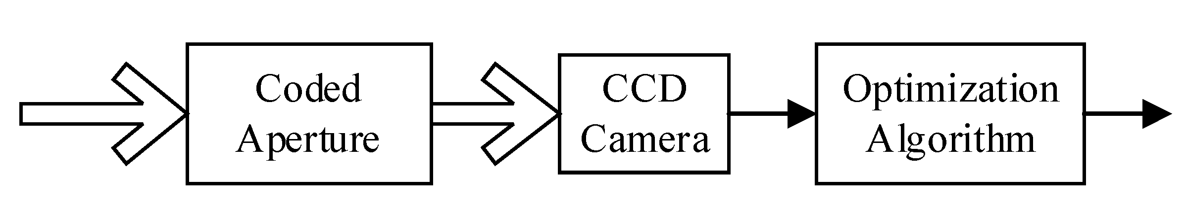
In the wavefront sensing section, the probe beam is passed through a programmable device that simulates a coded diffraction pattern (CDP) and then the intensity is measured by a charge-coupled device (CCD) camera and fed to a computer, which then optimizes it for calculation. The process is shown in Figure 3.

In the figure, ${\mathit{z}}_0$ is the initial value of the iteration, $y$ is the measured intensity value; $CDP(\cdot )$ represents the pattern after diffraction; $Az$ represents the measurement matrix; $*$ represents the multiply; and B is the intermediate value in the iterative calculation. After $ICDP(\cdot )$ solves the diffraction to find the gradient $grad$ and proceed to the next iteration, the final output is the calculated value $z$.

4. Analysis of Simulation Results

To verify the effectiveness of the MRWF algorithm proposed in this paper, experimental simulations of wavefront recovery are carried out in the MATLAB environment by simulating the transmission of vortex beams at different turbulence intensities. Atmospheric turbulence is simulated using equally spaced multi-phase screens, and the atmospheric turbulence model is fitted with Zernike polynomials for a total transmission distance of 1000 m, with adjacent phase screens spaced 100 m apart. The number of phase screen grids is 10, and the probe beam is chosen as a Gaussian beam, transmitted coaxially with the LG beam. The beam waist radius of the probe beam is 0.035 m and the beam waist radius of the information beam is 0.02 m, both at 1550 nm. The effect of turbulence intensity is expressed as a ratio of the atmospheric coherence length $r_0$ to the system aperture diameter $D$, where a larger $r_0$ indicates lower turbulence intensity. The specific parameter settings are shown in

Table 1. Parameter of simulation.

Parameter	Value
Laser wavelength λ	1550 nm
Width of phase screen D	0.3 m
Information beam waist w0	0.02 m
Topological charge l	3; 5; (2,3,5)
Turbulence intensity D/r0	0.2; 0.1; 0.02
Lateral offset d	0.1; 0.3; 0.5w0
Angular offset α	0.1; 0.2; 0.3λ/w0 rad
Transmission distance z	1 km
Number of phase screens	10

.

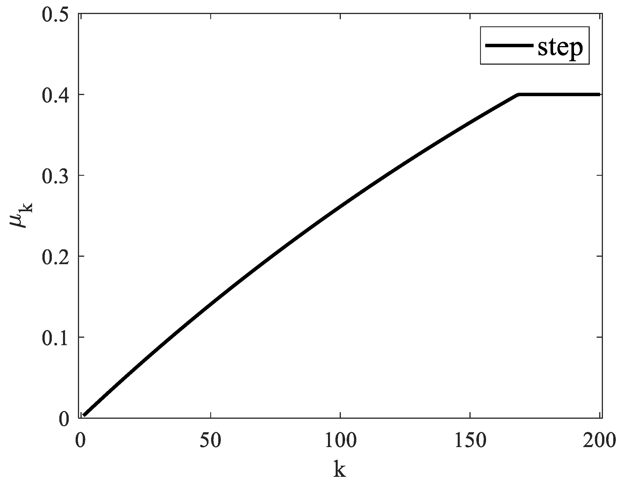
It is very easy to fall into a local optimum in non-convex optimization problems, and the MRWF algorithm suffers from this pitfall. A dynamic iteration step can effectively prevent it from falling into a local optimum solution, so this paper uses a heuristic variable-step-size method for gradient descent. When the iterations are first started, the iterative results differ significantly from the true values because of the high noise level, and a smaller step size can be set at this time. As the number of iterations increases, the result gets closer and closer to the true value, so a larger step size is chosen. When the result is close to the true value, the step size should be reduced again to prevent skipping the optimal value. The relationship between step size and number of iterations is shown in Figure 4.

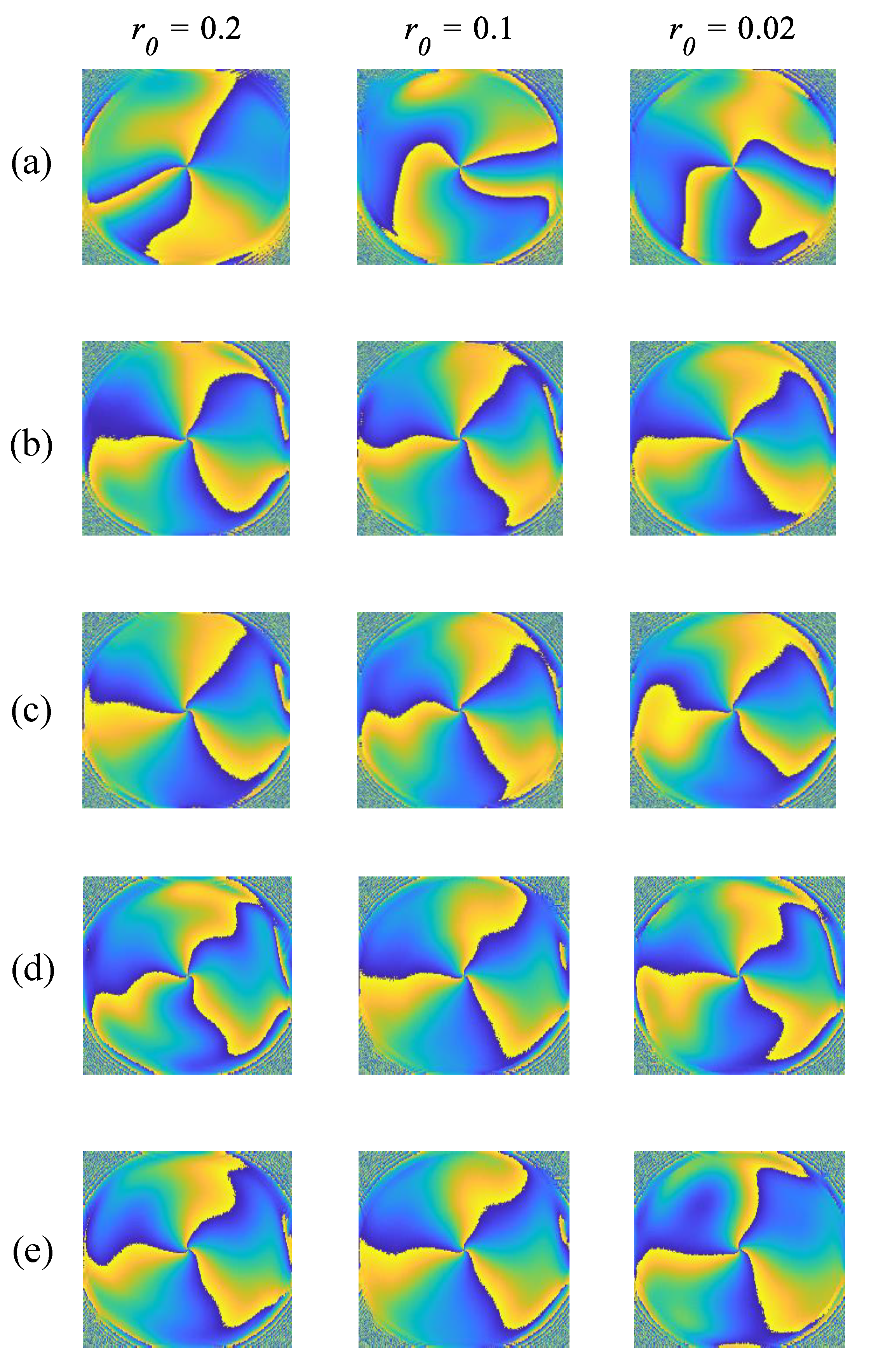
In order to verify the robustness of the MRWF algorithm, experiments were conducted to generate random turbulence phase screens at different turbulence intensities and to perform phase recovery by different algorithms for comparative experiments. An LG beam with a topological charge of 3 is chosen as the transmission beam and the atmospheric coherence lengths r₀ = 0.2 for weak turbulence, r₀ = 0.1 for moderate turbulence and r₀ = 0.02 for strong turbulence. The results are shown in Figure 5. Figure 5a shows the distorted phase after turbulence, Figure 5b shows the phase diagram of the LG beam after correction by the MRWF algorithm, Figure 5c shows the phase diagram of the LG beam after correction by the WF algorithm, Figure 5d shows the phase diagram of the LG beam after correction by the TWF algorithm and Figure 5e shows the phase diagram of the LG beam after correction by the RWF algorithm. As can be seen in Figure 5b,c, both the MRWF algorithm and the WF algorithm are effective in correcting the distorted wave front, but the MRWF algorithm achieves better recovery results than the WF algorithm in the case of strong turbulence. As can be seen in Figure 5b,d, the TWF algorithm also recovers the phase better, but the MRWF algorithm gives better recovery results than the TWF algorithm. As can be seen in Figure 5b,e, the MRWF algorithm recovers the phase better under various turbulent flows. The MRWF algorithm proposed in this paper has the performance advantage of successfully recovering the phase under different turbulent flows, and therefore the algorithm is robust under different turbulent intensities.

To further verify the robustness of the algorithm, experimental simulations were performed at different topological charge numbers, with the atmospheric coherence length $r_0=0.1$ and topological charge numbers set to 3, 5, {2, 3, 5}. The final results are shown in Figure 6. Figure 6a shows the distorted phase of the single-mode and multimode LG beams after turbulence, Figure 6b shows the phase diagram of the LG beam after correction by the MRWF algorithm, Figure 6c shows the phase diagram of the LG beam after correction by the WF algorithm, Figure 6d shows the phase diagram of the LG beam after correction by the TWF algorithm, and Figure 6e shows the phase diagram of the LG beam after correction by the RWF algorithm. It can be seen that both the MRWF algorithm and the conventional algorithm successfully correct the aberrated wavefront for both single-mode and multi-mode beams, so multi-mode does not affect the recovery results of the algorithm and the algorithm is more widely used. As can be seen in Figure 6b,c, both the MRWF algorithm and the WF algorithm are effective in correcting the distortion wavefront, but the MRWF algorithm has better recovery results than the WF algorithm. As can be seen in Figure 6b,d, the TWF algorithm is able to recover the phase, but its results are poor. As can be seen in Figure 6b,e, the two algorithms recover similar results and both recover the phase well. Next, the algorithm superiority will be verified by other evaluation metrics. In summary, the MRWF algorithm has strong robustness under different modalities.

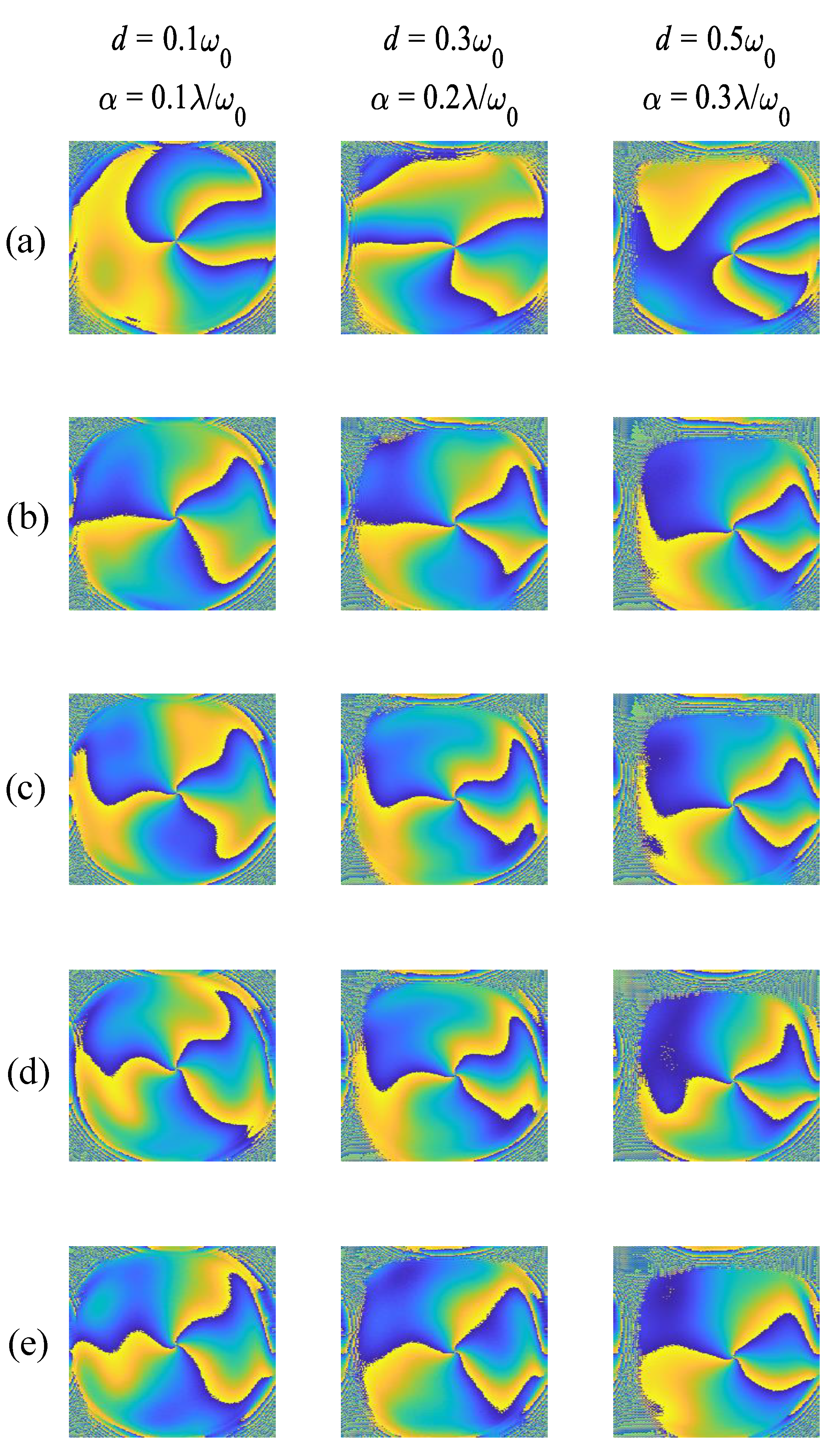
During space laser link communication, the signal light is transmitted over long distances to the optical receiving terminal, and due to pointing errors, the beam is offset at the receiving end, including lateral and angular offsets. The impact of pointing errors leads to a linear degradation in the performance of communication systems, so it is of practical importance to analyze systems affected by pointing errors. Fixing the effect of atmospheric turbulence r₀ = 0.1, with a topological charge of 3, the final simulation results are shown in Figure 7. Figure 7a shows the distorted phase after turbulence, Figure 7b shows the phase diagram of the LG beam after correction by the MRWF algorithm, Figure 7c shows the phase diagram of the LG beam after correction by the WF algorithm, Figure 7d shows the phase diagram of the LG beam after correction by the TWF algorithm and Figure 7e shows the phase diagram of the LG beam after correction by the RWF algorithm. As can be seen in Figure 7, the effect of pointing errors leads to more severe phase distortion and the performance of the phase recovery algorithm is limited. The MRWF algorithm recovers the phase closest to the ideal phase under the influence of different pointing errors. As the offset angle becomes larger, the isophotes are bent and distorted, at which point the MRWF algorithm is still the best recovery, followed by the RWF algorithm, with the TWF and WF algorithms coming close. Therefore, to better demonstrate the performance of the algorithm, SR and mode purity are next considered as evaluation metrics to validate the algorithm performance.

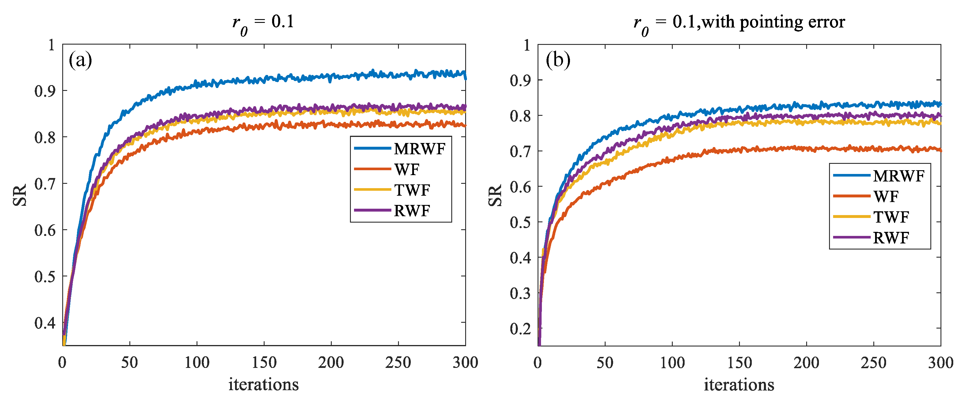
The phase of the LG beam is distorted due to the effects of turbulence. This distortion affects the orthogonality of the OAM modes, causing power loss in the modes and also causing inter-mode crosstalk, which affects the capacity and efficiency of the communication system. To further verify the effectiveness of the algorithm, simulation experiments were carried out from the SR parameters, setting r₀ = 0.1, lateral offset $d=0.3w_0$ and angular offset $\alpha =0.2\mathsf{\lambda }/w_0$, the results of which are shown in Figure 8. Figure 8a shows the recovery with atmospheric turbulence only, whereas Figure 8b shows the recovery with the combined effects of turbulence and pointing errors. As can be seen in Figure 8a, the MRWF algorithm has the best recovery for all different turbulence intensities, followed by the RWF algorithm. The TWF and MWF algorithms have similar recovery results, and the conventional WF algorithm has the worst results. The MRWF algorithm also requires a minimum number of iterations to reach the maximum recovery accuracy, which is usually achieved after 120 iterations. Using the MRWF algorithm, a recovered SR of 0.9 can be achieved at r₀ = 0.1. As can be seen in Figure 8b, the MRWF algorithm can achieve a recovered SR of 0.81 with the effect of pointing error, which is better than the other algorithms. After comparison, the MRWF algorithm has the strongest performance.

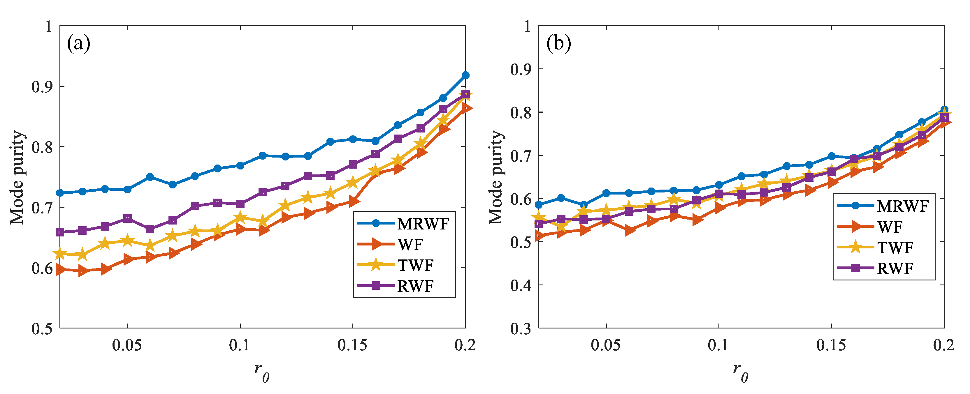
To further verify the effectiveness of the proposed algorithm, simulation experiments were carried out in terms of mode purity, setting the topological charge to 3, $r_0=0.02~0.2$, lateral offset $d=0.3w_0$ and angular offset $\alpha =0.2\mathsf{\lambda }/w_0$. The rest of the parameters remained unchanged, and the final results are shown in Figure 9. Figure 9a shows the recovery with only atmospheric turbulence and Figure 9b shows the recovery with the dual effect of turbulence and pointing error. It can be seen from Figure 9a that the MRWF algorithm has the highest recovered mode purity for different turbulence intensities. The mode purity can be recovered to over 0.9 for weak turbulence and over 0.7 for strong turbulence. As can be seen in Figure 9b, the overall recovery of the algorithm deteriorates for the case containing pointing errors, but is still optimal compared with the other algorithms. Therefore, it can be verified that the algorithm is valid from the recovery results of SR and mode purity.

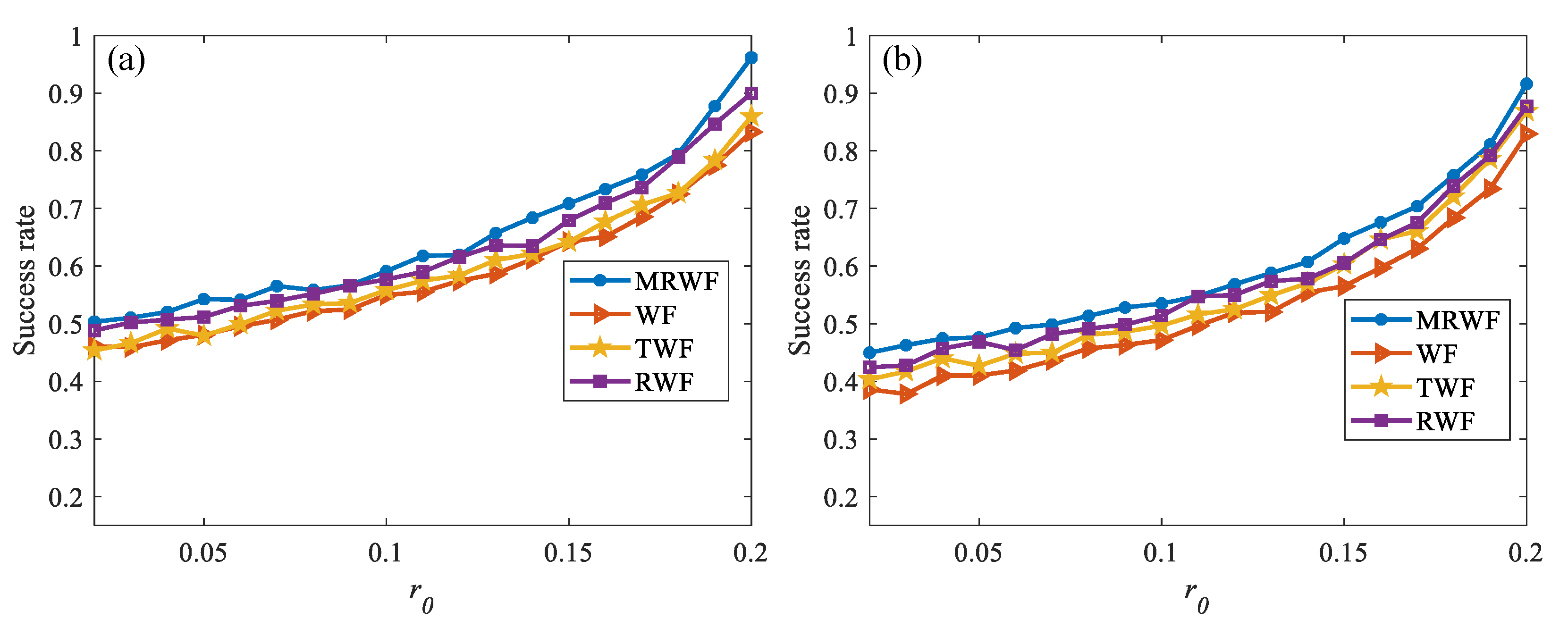
To verify the recovery success of the algorithm, set the topological load to 3, $r_0=0.02~0.2$, lateral offset $d=0.3w_0$ and angular offset $\alpha =0.2\mathit{\lambda }/w_0$. One thousand tests were carried out at each different turbulence intensity and success was judged to be when the root mean square error between the recovered phase and the true phase was less than 0.01. The results of the experiment are shown in Figure 10. Figure 10a shows the recovery with atmospheric turbulence only, whereas Figure 10b shows the recovery with the dual effect of turbulence and pointing error. As can be seen in Figure 10a,b, the MRWF algorithm has the best recovery success for different turbulence intensities or simulations containing pointing errors. The recovery success rate exceeds 90% in the case of weak turbulence and is close to 90% in the cases containing pointing errors, values that confirm the advantages of the MRWF algorithm for phase recovery.

5. Conclusions

In this paper, the conventional iterative phase recovery algorithm is investigated under the OAM-FSO communication system and an improved MRWF algorithm is proposed based on the WF algorithm. New initialization rules are first developed to take advantage of the stability of the median value in the sample and to eliminate the effect of outliers. A reweighting-based gradient descent method is then used to ensure that the iterative results are close to the true values. The MRWF algorithm is embedded in the wavefront sensing part of the adaptive optics system in conjunction with practical application scenarios. Finally, through simulation analysis, it is concluded that the MRWF algorithm is practically effective. Compared with the traditional WF algorithm and its variants, the MRWF algorithm gives the best recovery results, which are closest to the ideal values under the influence of different turbulences and different pointing errors. With the MRWF algorithm, the recovered SR can reach 0.9 at r₀ = 0.1 and with the influence of pointing errors, the MRWF algorithm can achieve a recovered SR of 0.81. In terms of mode purity, the MRWF algorithm achieves a recovered mode purity of 0.92 for weak turbulence and 0.72 for strong turbulence, and a recovered mode purity of 0.8 for pointing errors.