Image Quality Assessment for Digital Volume Correlation-Based Optical Coherence Elastography

 , and
, and 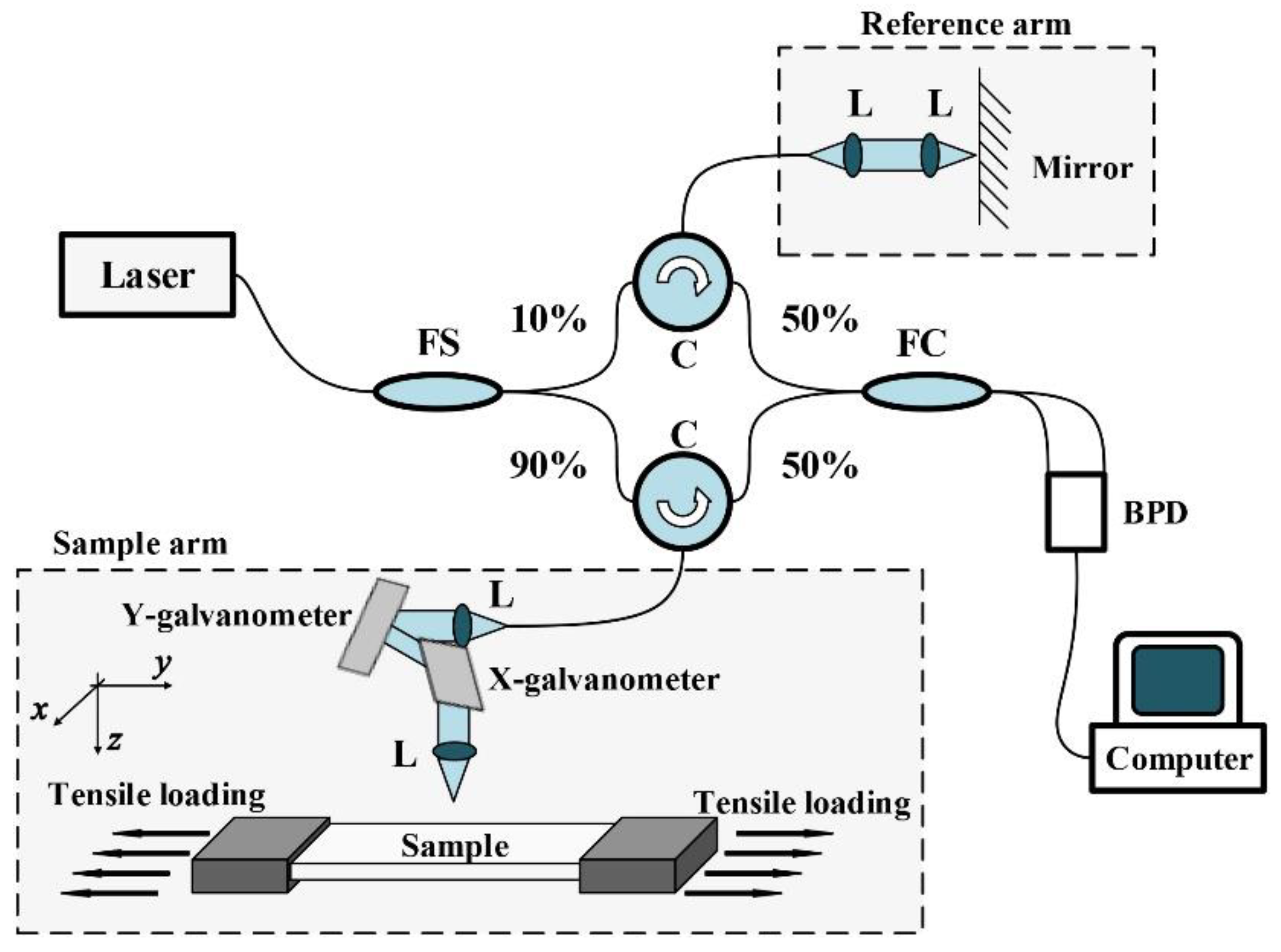
Abstract
1. Introduction
2. Materials and Methods
2.1. DVC-Based OCE
2.2. Quality Assessment of 3D OCT Images for DVC Calculation
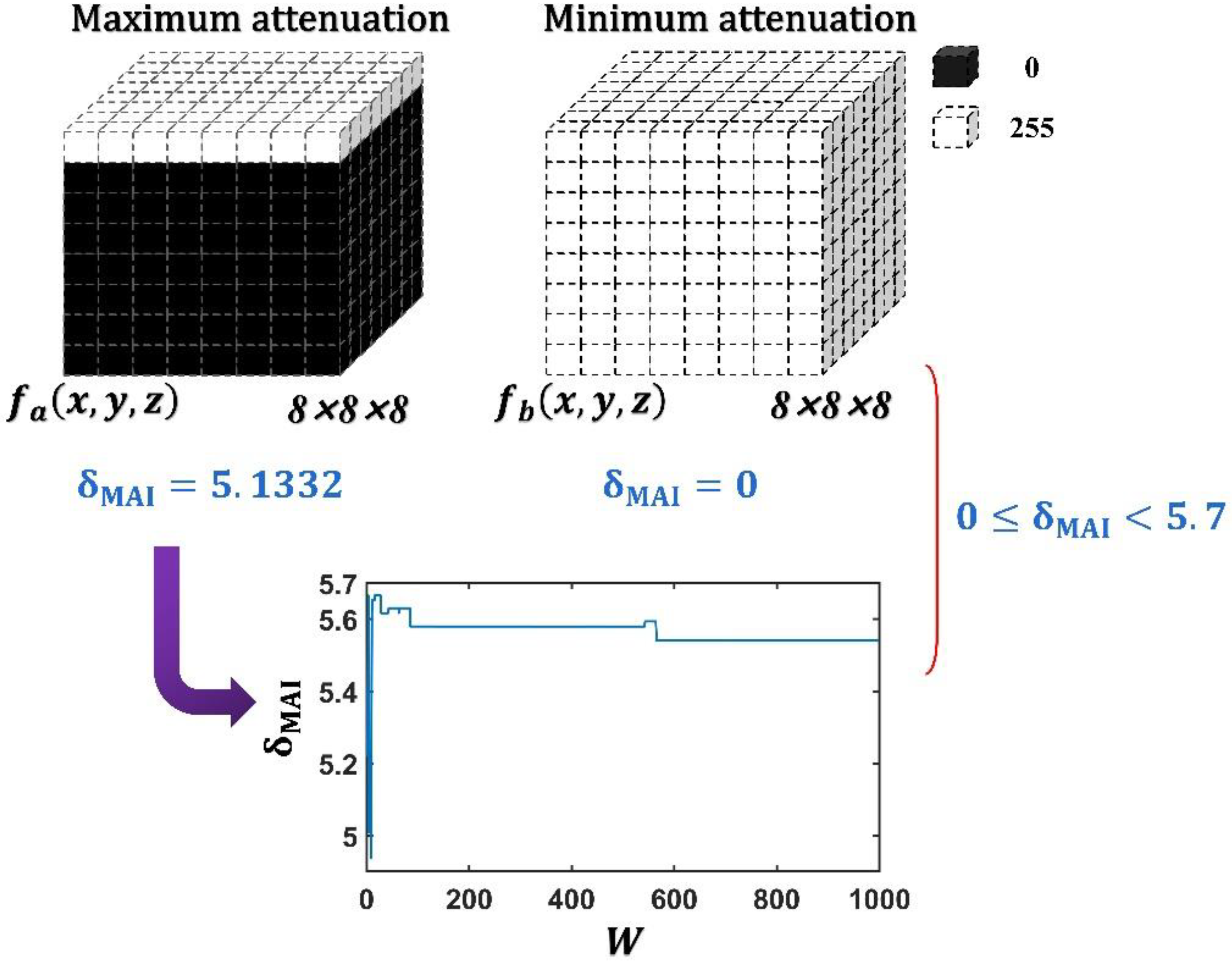
2.2.1. Mean Attenuation Intensity (MAI)
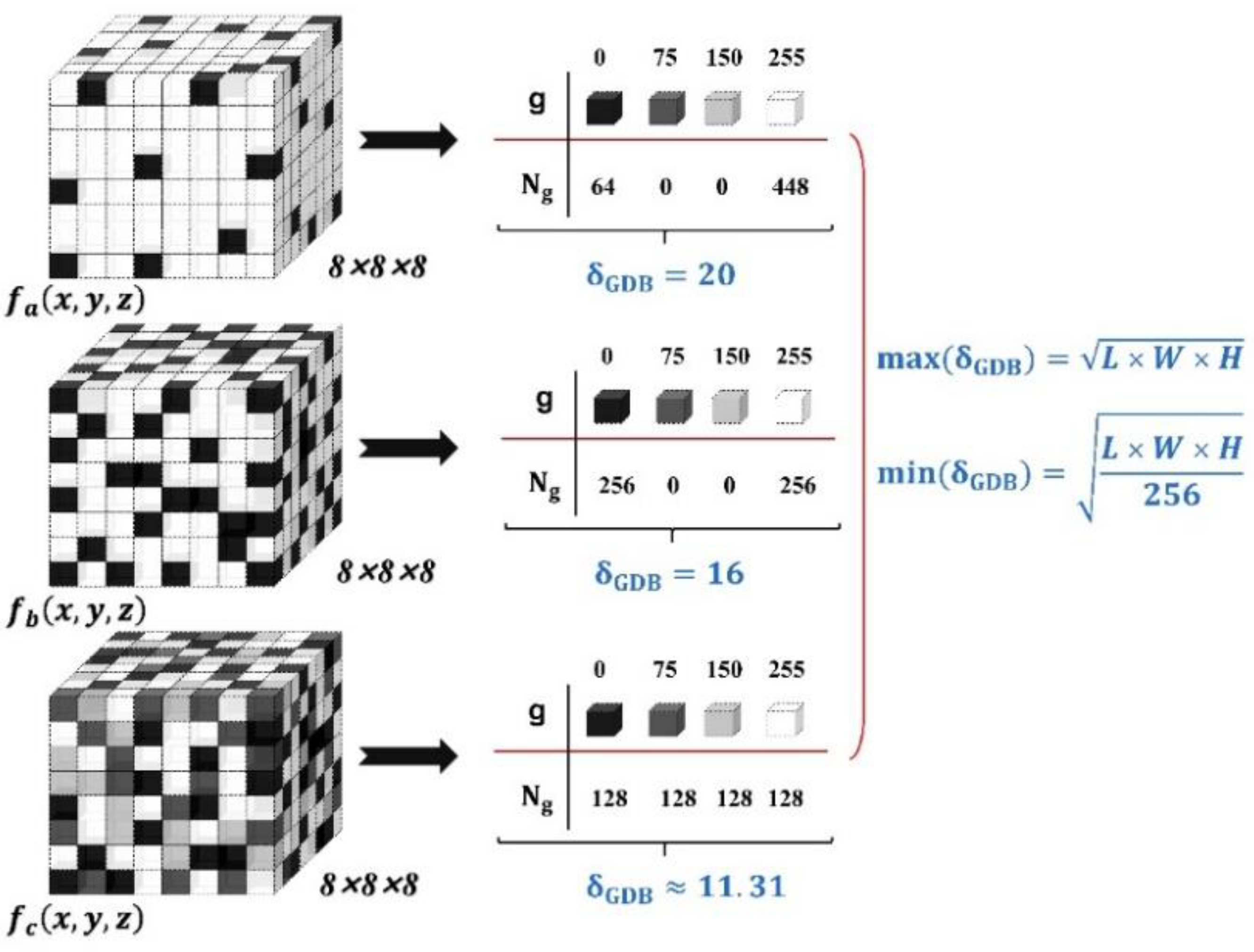
2.2.2. Breadth and Dispersion of the Gray Level Distribution
2.2.3. Image Evaluation Index Based on OCT-DVC
2.3. Mean Bias Error
3. Results
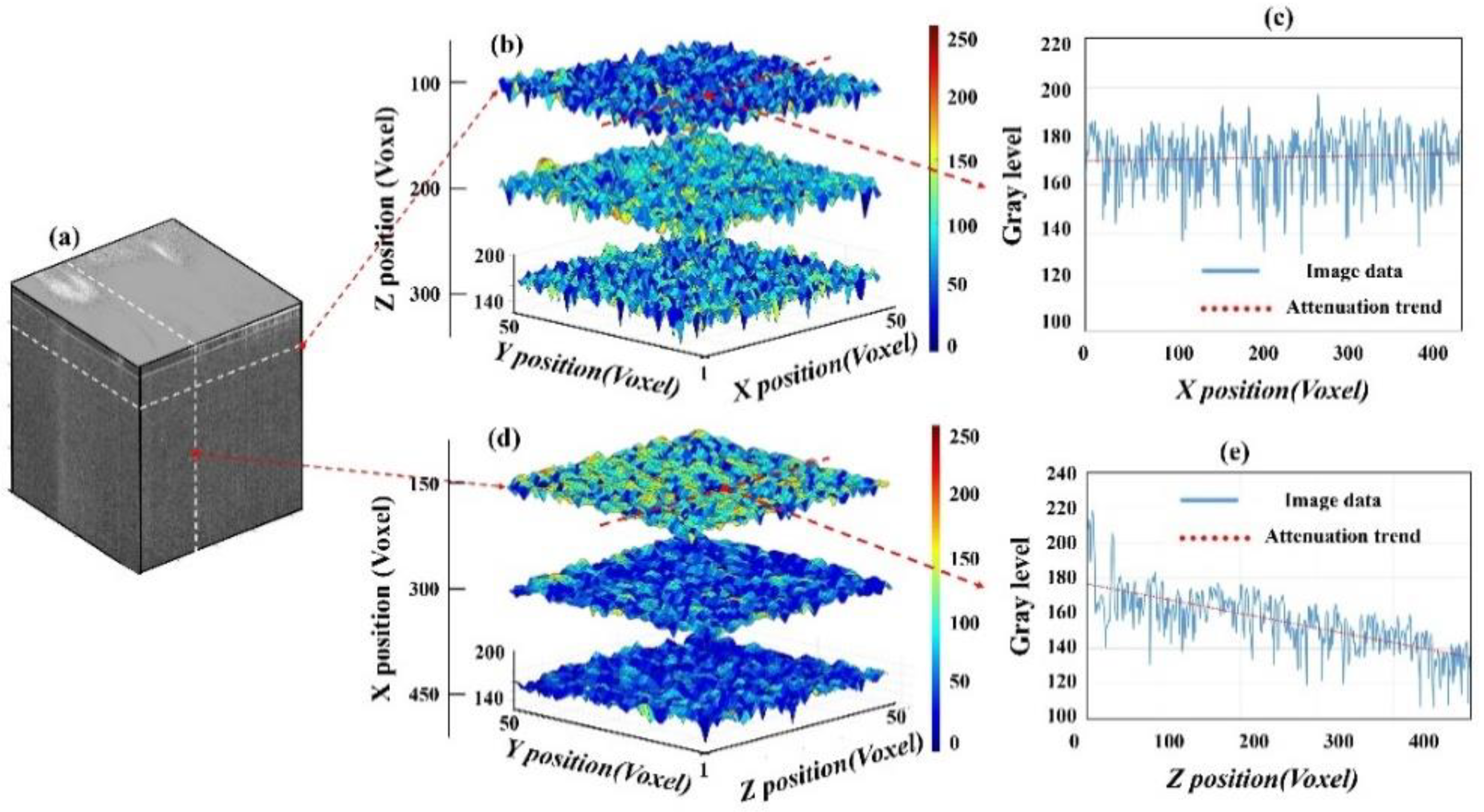
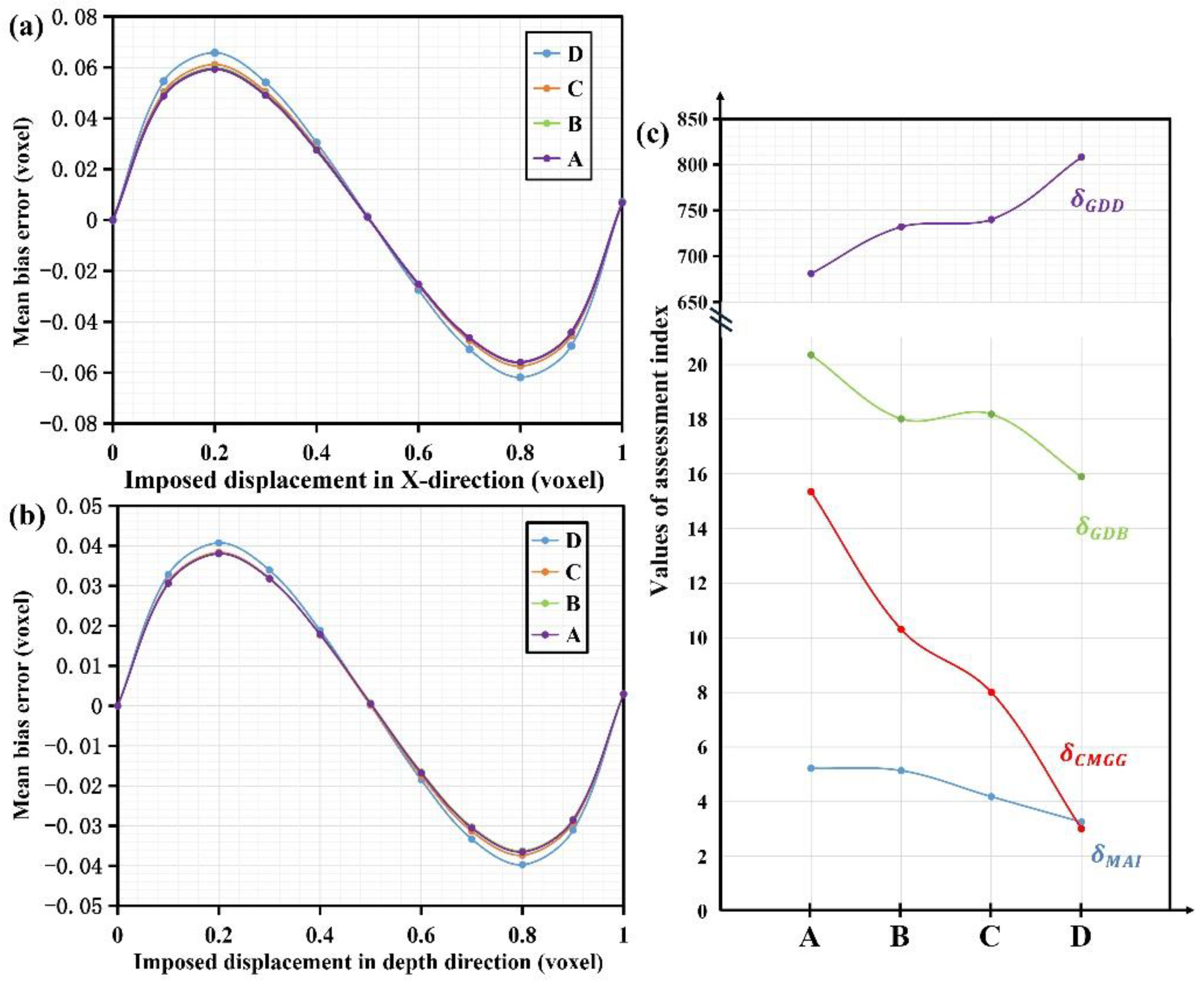
3.1. Verification Experiment of Reference Arm Adjustment
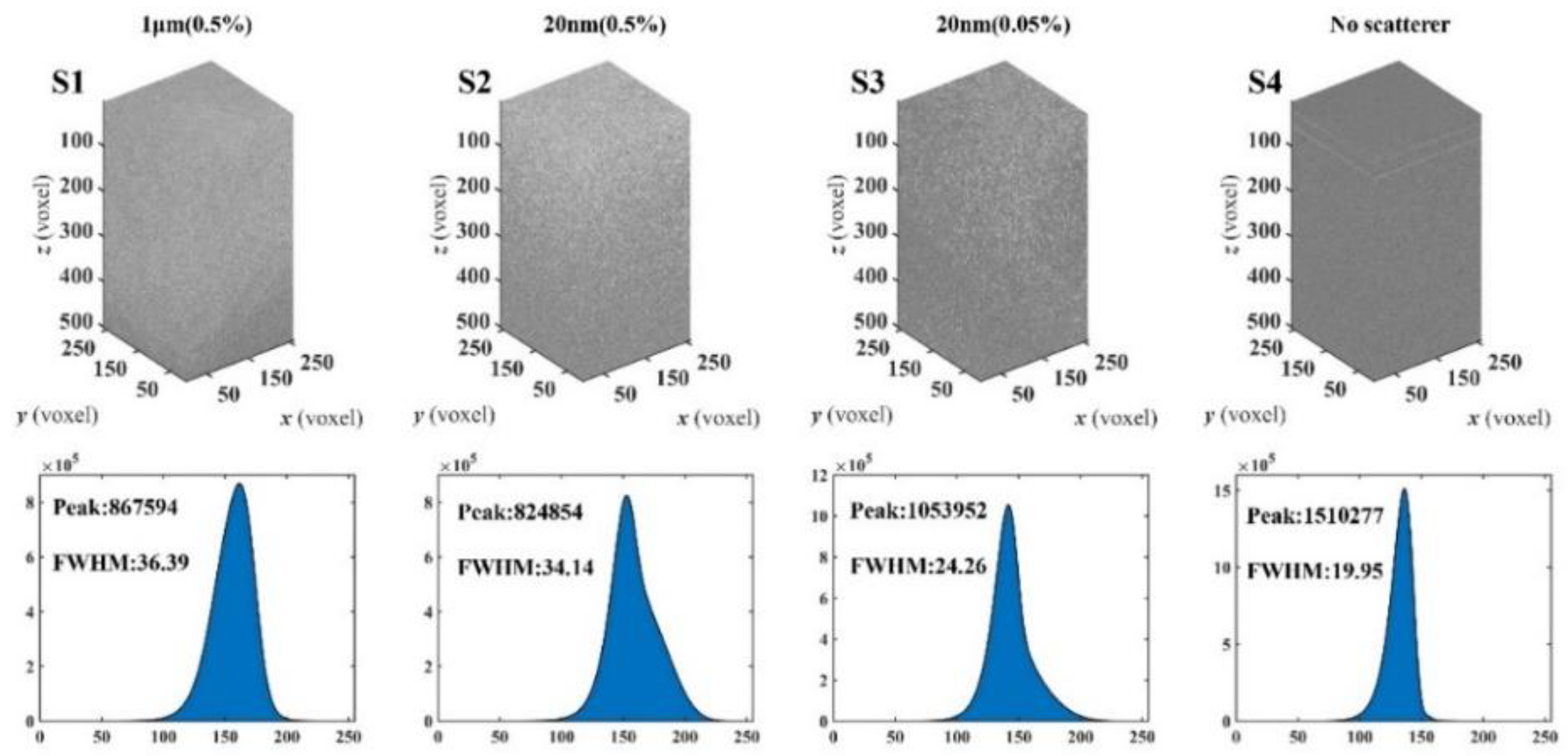
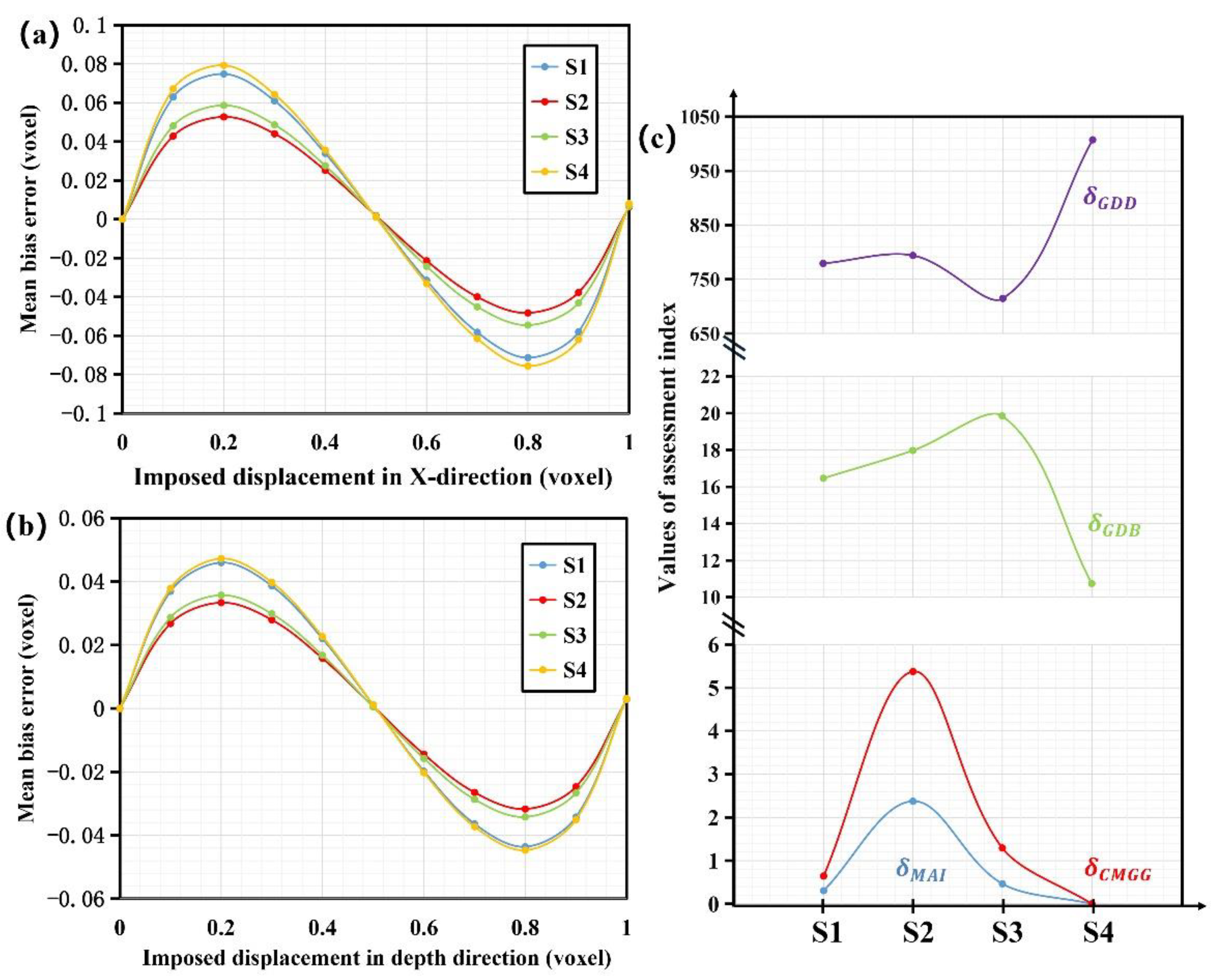
3.2. Verification Experiment of Phantoms with Different Scatterers
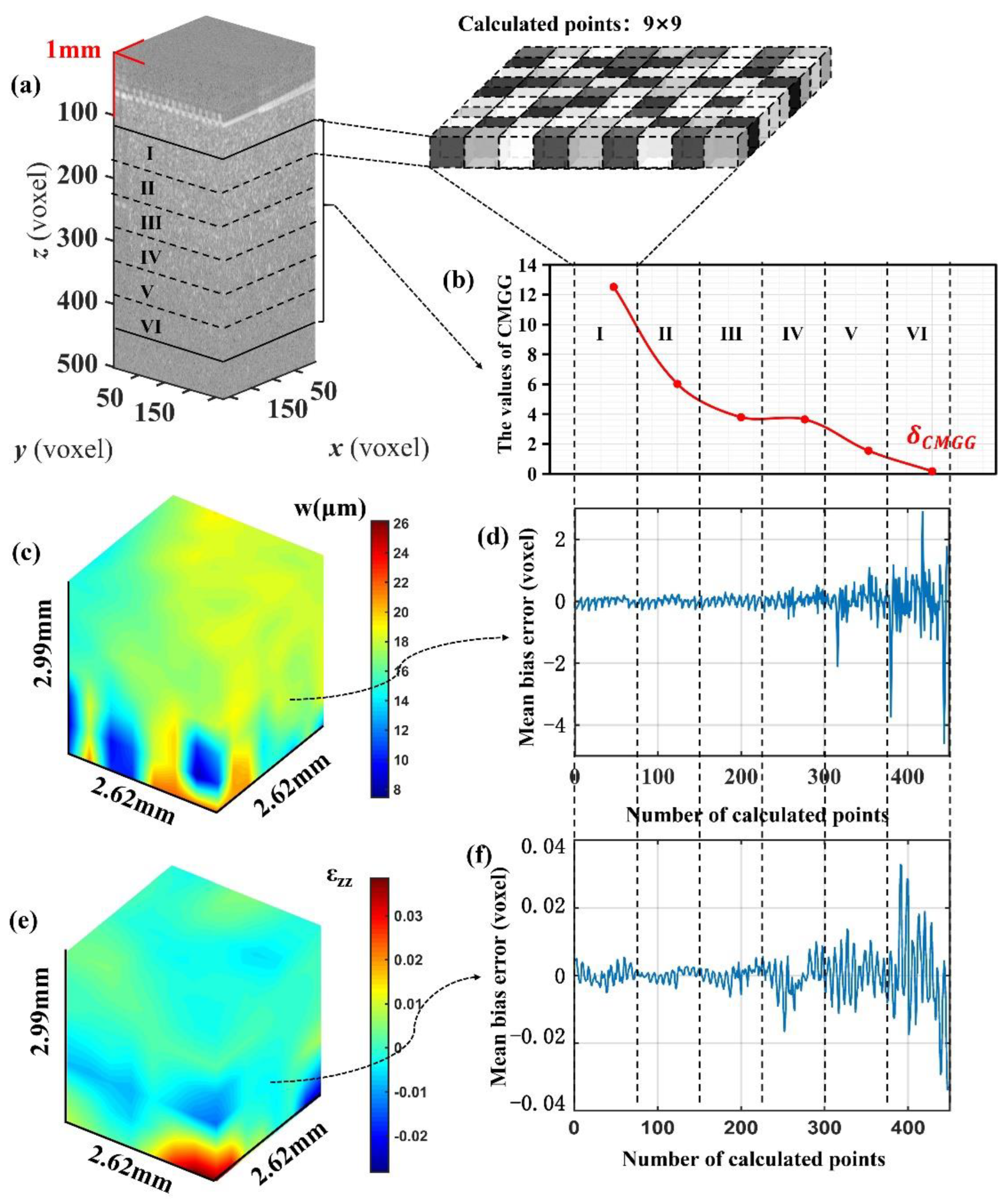
3.3. The Criteria Evaluation in Deformation Measurement of Pork Sample
4. Discussion
5. Conclusions
Author Contributions
Funding
Institutional Review Board Statement
Informed Consent Statement
Data Availability Statement
Acknowledgments
Conflicts of Interest
References
- Wang, S.; Larin, K.V. Optical coherence elastography for tissue characterization: A review. J. Biophotonics 2015, 8, 279–302. [Google Scholar] [CrossRef] [PubMed]
- Schmitt, J. OCT elastography: Imaging microscopic deformation and strain of tissue. Opt. Express 1998, 3, 199–211. [Google Scholar] [CrossRef] [PubMed]
- Ophir, J.; Céspedes, I.; Ponnekanti, H.; Yazdi, Y.; Li, X. Elastography: A Quantitative Method for Imaging the Elasticity of Biological Tissues. Ultrason. Imaging 1991, 13, 111–134. [Google Scholar] [CrossRef]
- Parker, K.J.; Doyley, M.M.; Rubens, D.J. Corrigendum: Imaging the elastic properties of tissue: The 20 year perspective. Phys. Med. Biol. 2012, 57, 5359–5360. [Google Scholar] [CrossRef][Green Version]
- Sun, C.; Standish, B.; Vuong, B.; Wen, X.Y.; Yang, V. Digital image correlation-based optical coherence elastography. J. Biomed. Opt. 2013, 18, 121515. [Google Scholar] [CrossRef] [PubMed]
- Fu, J.; Pierron, F.; Ruiz, P.D. Elastic stiffness characterization using three-dimensional full-field deformation obtained with optical coherence tomography and digital volume correlation. J. Biomed. Opt. 2013, 18, 121512. [Google Scholar] [CrossRef]
- Zaitsev, V.Y.; Matveyev, A.L.; Matveev, L.A.; Sovetsky, A.A.; Hepburn, M.S.; Mowla, A.; Kennedy, B.F. Strain and elasticity imaging in compression optical coherence elastography: The two-decade perspective and recent advances. J. Biophotonics 2021, 14, e202000257. [Google Scholar] [CrossRef]
- Larin, K.V.; Sampson, D.D. Optical coherence elastography-OCT at work in tissue biomechanics [Invited]. Biomed. Opt Express 2017, 8, 1172–1202. [Google Scholar] [CrossRef]
- Meng, F.; Chen, C.; Hui, S.; Wang, J.; Feng, Y.; Sun, C. Three-dimensional static optical coherence elastography based on inverse compositional Gauss-Newton digital volume correlation. J. Biophotonics 2019, 12, e201800422. [Google Scholar] [CrossRef]
- Santamaría, V.A.A.; Garcia, M.F.; Molimard, J.; Avril, S. Characterization of chemoelastic effects in arteries using digital volume correlation and optical coherence tomography. Acta Biomater. 2020, 102, 127–137. [Google Scholar] [CrossRef]
- Liu, P.; Groves, R.M.; Benedictus, R. Optical coherence elastography for measuring the deformation within glass fiber composite. Appl. Opt. 2014, 53, 5070–5077. [Google Scholar] [CrossRef] [PubMed][Green Version]
- Fu, J.; Haghighi-Abayneh, M.; Pierron, F.; Ruiz, P.D. Depth-Resolved Full-Field Measurement of Corneal Deformation by Optical Coherence Tomography and Digital Volume Correlation. Exp. Mech. 2016, 56, 1203–1217. [Google Scholar] [CrossRef]
- Midgett, D.E.; Quigley, H.A.; Nguyen, T.D. In vivo characterization of the deformation of the human optic nerve head using optical coherence tomography and digital volume correlation. Acta Biomater. 2019, 96, 385–399. [Google Scholar] [CrossRef]
- Ge, H.; He, Y.; Shen, L.; Liu, D.; Zhang, B.; Guo, S. Digital image frequency spectrum method for analyzing speckle displacement in frequency domain. Opt. Lett. 2015, 40, 942–945. [Google Scholar] [CrossRef] [PubMed]
- Schreier, H.W.; Sutton, M.A. Systematic errors in digital image correlation due to undermatched subset shape functions. Exp. Mech. 2002, 42, 303–310. [Google Scholar] [CrossRef]
- Schreier, H.; Braasch, J.; Sutton, M. Systematic errors in digital image correlation caused by intensity interpolation. Opt. Eng. 2000, 39, 2915–2921. [Google Scholar] [CrossRef]
- Gossage, K.W.; Smith, C.M.; Kanter, E.M.; Hariri, L.P.; Stone, A.L.; Rodriguez, J.J.; Williams, S.K.; Barton, J.K. Texture analysis of speckle in optical coherence tomography images of tissue phantoms. Phys. Med. Biol. 2006, 51, 1563–1575. [Google Scholar] [CrossRef][Green Version]
- Pan, Y.; Birngruber, R.; Engelhardt, R. Contrast limits of coherence-gated imaging in scattering media. Appl. Opt. 1997, 36, 2979–2983. [Google Scholar] [CrossRef]
- Bashkansky, M.; Reintjes, J. Statistics and reduction of speckle in optical coherence tomography. Opt. Lett. 2000, 25, 545–547. [Google Scholar] [CrossRef]
- Iftimia, N.; Bouma, B.E.; Tearney, G.J. Speckle reduction in optical coherence tomography by path length encoded angular compounding. J. Biomed. Opt. 2003, 8, 260. [Google Scholar] [CrossRef]
- Rogowska, J.; Bryant, C.M.; Brezinski, M.E. Cartilage thickness measurements from optical coherence tomography. J. Opt. Soc. Am. A 2003, 20, 357–367. [Google Scholar] [CrossRef] [PubMed]
- Pircher, M.; Gotzinger, E.; Leitgeb, R.; Fercher, A.F.; Hitzenberger, C.K. Speckle reduction in optical coherence tomography by frequency compounding. J. Biomed. Opt. 2003, 8, 565–569. [Google Scholar] [CrossRef] [PubMed]
- Tyler, S.; Ralston; Daniel, L.; Marks; Scott, P.; Carney; Stephen, A.; Boppart. Real-time interferometric synthetic aperture microscopy. Opt. Express 2008, 16, 4. [Google Scholar] [CrossRef]
- Matveyev, A.L.; Matveev, L.A.; Moiseev, A.A.; Sovetsky, A.A.; Gelikonov, G.V.; Zaitsev, V.Y. Semi-analytical full-wave model for simulations of scans in optical coherence tomography with accounting for beam focusing and the motion of scatterers. Laser Phys. Lett. 2019, 16, 085601. [Google Scholar] [CrossRef]
- Zaitsev, V.Y.; Matveyev, A.L.; Matveev, L.A.; Gelikonov, G.V.; Gelikonov, V.M.; Vitkin, A. Deformation-induced speckle-pattern evolution and feasibility of correlational speckle tracking in optical coherence elastography. J. Biomed. Opt. 2015, 20, 75006. [Google Scholar] [CrossRef]
- Pan, B.; Lu, Z.; Xie, H. Mean intensity gradient: An effective global parameter for quality assessment of the speckle patterns used in digital image correlation. Opt. Lasers Eng. 2010, 48, 469–477. [Google Scholar] [CrossRef]
- Yu, H.; Guo, R.; Xia, H.; Yan, F.; Zhang, Y.; He, T. Application of the mean intensity of the second derivative in evaluating the speckle patterns in digital image correlation. Opt. Lasers Eng. 2014, 60, 32–37. [Google Scholar] [CrossRef]
- Bomarito, G.F.; Hochhalter, J.D.; Ruggles, T.J.; Cannon, A.H. Increasing accuracy and precision of digital image correlation through pattern optimization. Opt. Lasers Eng. 2017, 91, 73–85. [Google Scholar] [CrossRef]
- Song, J.; Yang, J.; Liu, F.; Lu, K. Quality assessment of laser speckle patterns for digital image correlation by a Multi-Factor Fusion Index. Opt. Lasers Eng. 2020, 124, 105822. [Google Scholar] [CrossRef]
- Karamata, B.; Hassler, K.; Laubscher, M.; Lasser, T. Speckle statistics in optical coherence tomography. J. Opt. Soc. Am. A 2005, 22, 593–596. [Google Scholar] [CrossRef]
- Armitage, J.; Lamouche, G.; Vergnole, S.; Bisaillon, C.E.; Dufour, M.; Maciejko, R.; Monchalin, J.P. Speckle size in optical Fourier domain imaging. In Photonics North; SPIE: Bellingham, DC, USA, 2007. [Google Scholar]
- Lee, P.; Gao, W.; Zhang, X. Speckle properties of the logarithmically transformed signal in optical coherence tomography. J. Opt. Soc. Am. A 2011, 28, 517–522. [Google Scholar] [CrossRef] [PubMed]
- Gong, P.; Almasian, M.; van Soest, G.; de Bruin, D.; van Leeuwen, T.; Sampson, D.; Faber, D. Parametric imaging of attenuation by optical coherence tomography: Review of models, methods, and clinical translation. J. Biomed. Opt. 2020, 25, 040901. [Google Scholar] [CrossRef] [PubMed]
- Puvanathasan, P.; Bizheva, K.J.O.E. Interval type-II fuzzy anisotropic diffusion algorithm for speckle noise reduction in optical coherence tomography images. Opt. Express 2009, 17, 733–746. [Google Scholar] [CrossRef] [PubMed]
- Meng, F.; Zhang, X.; Wang, J.; Li, C.; Chen, J.; Sun, C. 3D Strain and Elasticity Measurement of Layered Biomaterials by Optical Coherence Elastography based on Digital Volume Correlation and Virtual Fields Method. Appl. Sci. 2019, 9, 1349. [Google Scholar] [CrossRef]
- Su, Y.; Zhang, Q.; Gao, Z. Statistical model for speckle pattern optimization. Opt. Express 2017, 25, 30259–30275. [Google Scholar] [CrossRef] [PubMed]
- Silva, V.B.; Andrade De Jesus, D.; Klein, S.; van Walsum, T.; Cardoso, J.; Brea, L.S.; Vaz, P.G. Signal-carrying speckle in optical coherence tomography: A methodological review on biomedical applications. J. Biomed. Opt. 2022, 27, 030901. [Google Scholar] [CrossRef] [PubMed]


Publisher’s Note: MDPI stays neutral with regard to jurisdictional claims in published maps and institutional affiliations. |
© 2022 by the authors. Licensee MDPI, Basel, Switzerland. This article is an open access article distributed under the terms and conditions of the Creative Commons Attribution (CC BY) license (https://creativecommons.org/licenses/by/4.0/).
Share and Cite
Lin, X.; Chen, J.; Hu, Y.; Feng, X.; Wang, H.; Liu, H.; Sun, C. Image Quality Assessment for Digital Volume Correlation-Based Optical Coherence Elastography. Photonics 2022, 9, 573. https://doi.org/10.3390/photonics9080573
Lin X, Chen J, Hu Y, Feng X, Wang H, Liu H, Sun C. Image Quality Assessment for Digital Volume Correlation-Based Optical Coherence Elastography. Photonics. 2022; 9(8):573. https://doi.org/10.3390/photonics9080573
Chicago/Turabian StyleLin, Xianglong, Jinlong Chen, Yongzheng Hu, Xiaowei Feng, Haosen Wang, Haofei Liu, and Cuiru Sun. 2022. "Image Quality Assessment for Digital Volume Correlation-Based Optical Coherence Elastography" Photonics 9, no. 8: 573. https://doi.org/10.3390/photonics9080573
APA StyleLin, X., Chen, J., Hu, Y., Feng, X., Wang, H., Liu, H., & Sun, C. (2022). Image Quality Assessment for Digital Volume Correlation-Based Optical Coherence Elastography. Photonics, 9(8), 573. https://doi.org/10.3390/photonics9080573