Novel Elastography-Inspired Approach to Angiographic Visualization in Optical Coherence Tomography

Abstract

In this paper, we present a new approach to contrast-agent-free angiographic visualization in optical coherence tomography (OCT). The proposed approach has much in common with imaging of local interframe strains in OCT-based elastography and utilizes the fact that the interframe motion of blood particles leads to discontinuity of strains within the vessel cross section. By this reasoning, we call this approach “elastography-inspired”. Here, we first elucidate the essence and main features of the elastography-inspired approach using numerical simulation of OCT data. The simulations allow one to introduce both moving scatterers imitating blood flow in vessels as well as various masking motions imitating natural motions of living “solid” tissue surrounding the vessels. Second, using real OCT signals, we present comparative results of angiographic processing using the proposed elastography-inspired approach and a realization of OCA based on high-pass filtering of temporal variability of a series of OCT B-scans. The two methods can use the same initial dataset and the high-pass filtering OCA has already been routinely applied in both animal experiments and on patients. The new elastography-inspired method has a similar computational efficiency, and it is intrinsically able to compensate spatially-inhomogeneous masking tissue motions and demonstrates high robustness with respect to motion artefacts. Thus, the new approach looks very promising for enabling wider application of OCA in both laboratory studies on animals and, most importantly, for wider clinical applications on patients.

1. Introduction

One of the main trends in the development of OCT in recent years is the emergence of various functional extensions (modalities) beyond structural visualization of biological tissues [1]. Optical coherence angiography (OCA) is one such functional extension. Basically, various realizations of OCA enable visualization of the blood-vessel network using blood particles’ own motions. This motion of the blood flow makes it possible to discriminate the vessels from the surrounding “solid” motionless tissue. A variety of methods of numerical processing of OCT signals enable angiographic visualization. In particular, some methods use the Doppler effect [2,3,4], although the Doppler frequency shift is fairly small (in the order of several kHz for typical blood-flow velocities of the order of mm/s in small vessels visualized by OCT) in comparison with optical frequency ~10¹⁴ Hz. Due to this, the Doppler frequency shift is estimated indirectly using the measured phase shift between the compared OCT signals obtained with a known time delay. The Doppler shift does not occur if the signal is scattered by the “solid” motionless tissue outside the vessel cross section. Thus, using the evaluation of Doppler shift, the images of blood vessels can be constructed, and even the blood-flow velocity and its direction can be estimated.

There are other approaches in which the signal phase is not used and only the variations in the amplitude or intensity are analyzed [5]. One of such approaches, termed speckle-variance (SV) OCA [6], uses analysis of a series of OCT scans obtained in the same position. The pixels corresponding to the motionless tissue do not change their intensity (and exhibit low-level variance), whereas the pixels corresponding to the vessel cross-sections demonstrate locally increased variance, due to which the vessel cross sections can be discriminated and the micro-vessel network can be reconstructed. This principle is easier for realization than the Doppler approach, although, in the SV-method, the blood-flow velocity is not evaluated. Rather, the vessel-network geometry is reconstructed nearly independently of the direction of the flow [7]. Another way to discriminate cross sections of vessels from the “solid” tissue, which is also based on amplitude (intensity) variability, is the utilization of cross-correlation of the spatial patterns in the compared OCT scans consequently acquired for the same position [8]. There are also a number of OCA realizations in which complex-valued OCT signals are analyzed using the temporal variability of both signal amplitude and phase [9].

In the context of various approaches that are used to single out temporal variability, among the most popular methods are differential operations [10] and evaluation of temporal decorrelation for a series of sequential OCT scans acquired for the same position [11,12,13].

One more method of singling out temporal variability of OCT-data in cross sections of blood vessels was proposed in [14] using the high-pass (HP) filtering approach. An important distinction in the realization of this approach is that instead of a conventionally used comparison of OCT scans acquired for the same position, in the HP-filtering approach, the compared scans are obtained using a slowly moving illuminating beam, which is sufficiently self-overlapping. In comparison with acquiring repeated OCT signals for the same position with step-wise switching to the next position, the utilization of a slowly moving scanning beam significantly simplifies the beam-motion control due to elimination of transitional processes that are typical of step-wise changes in the beam position. Elimination of the transitional processes is also favorable for shortening the time of acquisition of 3D signal sets.

Certainly, because the illuminating beam is moving (albeit slowly), the signal for motionless “solid” tissue also exhibits some variability. However, in the vessel cross section, this variability is even faster, so that for the properly chosen parameters of the HP filtering, it is possible to discriminate the contribution of sufficiently slow varying signals from the “solid” tissue and selectively retain the faster-varying signals from the vessel cross sections. The self-overlapping of the illuminating beam may be realized in various directions. One variant of significantly overlapping neighboring A-scans within one B-scan was described in [14]. In [15], a modified variant of the HP-filtering approach was reported in which, instead of the strong overlapping of A-scans within every single B-scan, an entire 3D dataset was acquired with a significant overlap of neighboring B-scans. In practice, the step between B-scans can be about 1/7–1/10 of the illuminating-beam diameter, which is sufficient for singling out the vessels by using the HP-filtering.

Since it makes no sense to compare signals in B-scans that are not overlapped, it makes no sense to initially acquire the entire 3D data volume and only then perform the HP-filtering through the total thickness of the data stack along the slow-scanning direction. In this regard, visualization of vessels by HP-filtering implies such stages as forward Fourier transform, filtering procedure in the Fourier domain and then inverse Fourier transform to obtain the image in the spatial domain. According to the Fourier transform properties, these three stages are equivalent to a single convolution procedure (along the slow-scanning direction) of the initial OCT data with a kernel function, the spectrum of which corresponds to the shape of the HP-filtering window. An important requirement is that the length of this kernel function should cover the stack of the self-overlapped B-scans. Performing such a convolution with a gradual shift of the kernel function makes it possible to visualize the vessels on-flight without the necessity to acquire the entire 3D-stack, consisting of several hundred B-scans [15]. Unlike post-processing-based OCA methods, such on-flight visualization of vessels allows one to control the quality of the acquired image in real time and, therefore, avoid collection of fully corrupted data, e.g., by the own masking motions of living tissues.

It should be emphasized that the degrading role of living-tissue motions is a critical point for all contrast-agent-free angiographic approaches in which the own motion of blood particles is used as a contrast mechanism. However, in reality, even the “solid” tissue surrounding the vessels is not static at all, but performs various motions caused by heart-beating, breathing, etc. The velocity/amplitude of such motions may be even greater than for blood-particle motions, although the latter is supposed to be distinguishable from the masking motions of the “solid” tissue. In view of this, various methods enabling physical immobilization of the examined tissue and/or compensation of masking motions by appropriate signal processing are required for operability of all types of contrast-agent-free OCA methods.

In particular, for tissue stabilization in animal experiments, immobilizing dorsal chambers with transparent windows is often used [16]. Additionally, the research in [14] proposed compensation of translational motions by correcting the depth-averaged phases of overlapping A-scans. For visualizing retinal blood flow, eye-ball immobilization, which is often required for other ophthalmic procedures, may be favorable for OCA visualization as well.

However, for non-ophthalmic applications on patients, immobilizing devices/chambers usually are not acceptable. At the same time, translational motions that are typical of non-contact examinations often are too strong to be numerically compensated. In view of this, in the above-mentioned approach [15], instead of a non-contact regime, it was proposed to use a contact regime for OCA examinations, which opens the way for its application on animals without the necessity of immobilizing chambers (as in [17,18]) and even on patients without additional mechanical fixation [19,20]. The contact between the OCT output window and tissue is minimally invasive (to the same degree as ultrasound examinations) and, for this reason, in many cases, it can be used on patients. At the same time, the contact mode efficiently eliminates large-scale motions that are typical of non-contact examinations of living organisms, including patients, which is an important advantage of contact-mode OCA.

Although the contact mode eliminates large-scale translational motions typical of a non-contact regime, the compression applied to the tissue by the contacting OCT probe produces strains. Consequently, scatterers in the tissue experience depth-dependent motions that also produce the masking effect and degrade the contrast between the “solid” tissue and blood vessels. Compensation for such depth-dependent motions significantly differs and requires more complex signal processing than depth-independent translational motions [15].

It should be emphasized that for all realizations of OCA approaches, the problem of efficient elimination of masking tissue motions remains challenging. Another closely related important point is the possibility of enabling OCA visualization in real time. For solving this problem, the number of compared OCT scans should be minimized and the OCA processing should be sufficiently computationally efficient.

To contribute to a solution for the above-mentioned problems, in this paper, we propose a new method of OCT-based angiographic visualization. It is essentially different from all realizations of OCA oriented to the usage of temporal variability of OCT signal in the cross section of blood vessels. In the new approach, we propose to utilize the fact of occurrence of the blood flow rather in a local vessel cross section, where the motion of blood particles is essentially independent of the motion of scatterers in the surrounding “solid” tissue. For the latter, the deformations obey the mechanics of continua and, therefore, strains produced in the tissue by the contacting OCT-probe are continuous. On the contrary, due to the independent motion of blood particles in the cross sections of vessels, in the OCT-scan plane, the continuity of deformations in the vessel cross sections is broken. Thus, the vessel cross section can be discriminated as local discontinuities of strain against a fairly smooth strain field corresponding to the background tissue.

For realization of this idea, one can apply the efficient methods of visualization of local strains for utilization in OCT-based elastography, developed in recent years [21]. Due to this close relation to the OCT elastography, the proposed OCA method is reasonably referred to as “elastography-inspired”. This idea of visualization of a vessel’s cross section as spots of discontinuities in the strain distribution is attractive for utilization in the contact-mode OCA, for which the compression-produced spatially-inhomogeneous masking displacements of scatterers in the “solid” tissue represent a serious challenge for OCA algorithms based on the evaluation of temporal variability of particle motions.

In what follows, we first describe how the proposed OCA algorithm can be realized using the efficient “vector” approach for visualization of local strains. Then, we will demonstrate the operability of the elastography-inspired OCA method using numerically simulated OCT signals imitating the presence of a vessel in the surrounding tissue that experiences compression-produced strains. Finally, we present an example of such elastography-inspired OCA using real OCT signals and compare its results with the OCA imaging based on HP-filtering [15] using the same data obtained for a labial mucosa of a volunteer.

2. Materials and Methods

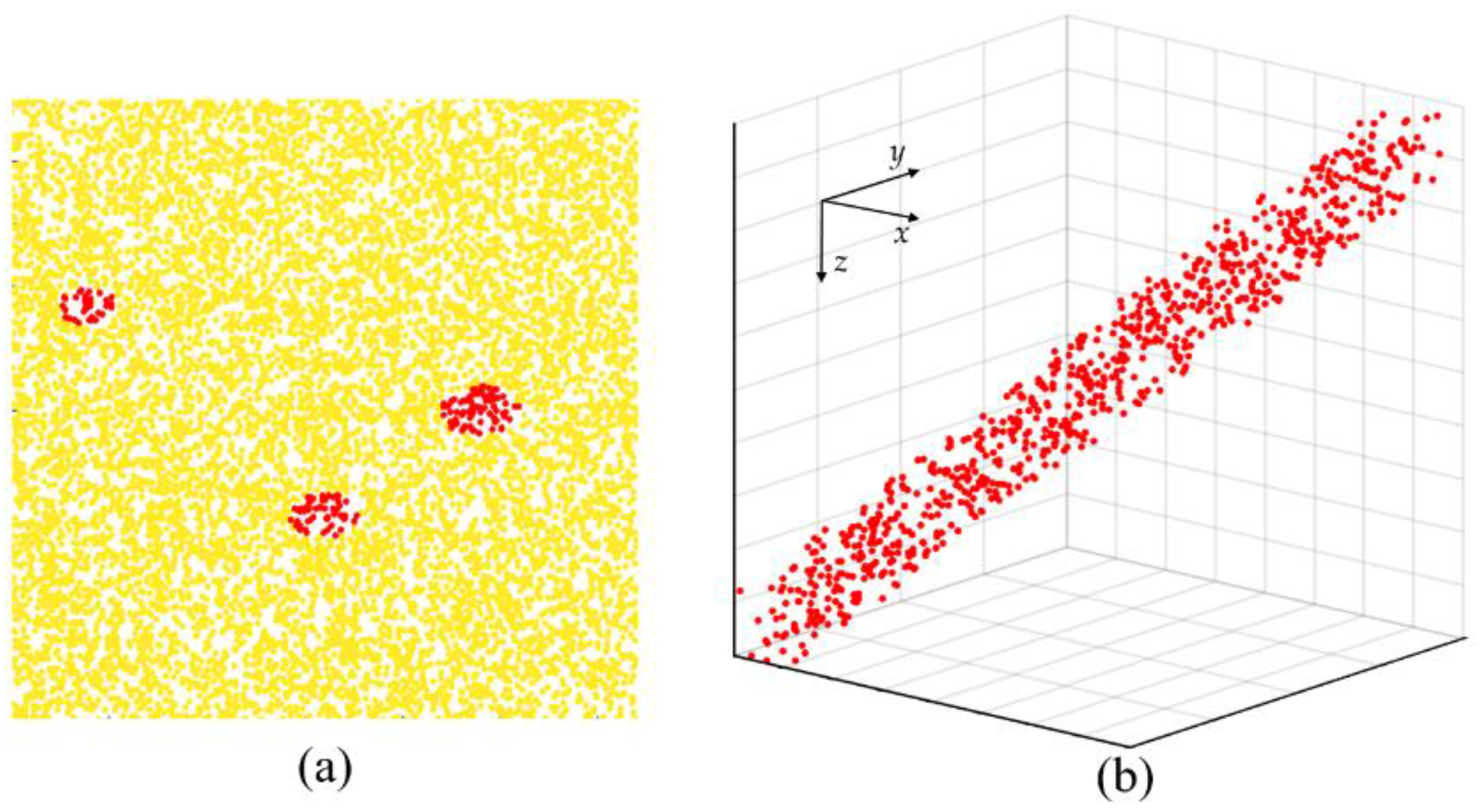
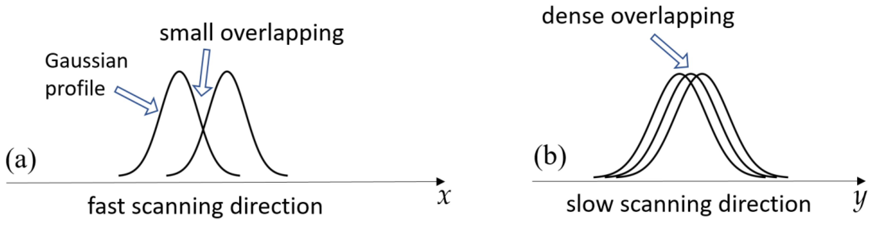
2.1. Method of Simulation of OCT-Scans with Arbitrary Motion of Scattering Particles

In this study, for demonstration of the proposed elastography-inspired OCA method and comparison of the HP-filtering OCA algorithm, for which the same scanning pattern can be used, first we will use simulated OCT images. There are numerous known approaches to simulating OCT scans, in particular, Monte-Carlo methods [22,23,24]. However, usually, such models are not well adapted to account for moving scatterers, which is indispensable for simulating the blood flow. Due to this reason, in the simulations we use the simulation approach described in our previous works [25,26]. This approach utilizes the widely used approximation of discrete scatterers (in general, similar to work [27]). The approach used is based on the approximation of ballistic scattering from a set of localized discrete scatterers that can experience arbitrary displacements between the consequently formed OCT scans. Due to this ability, the model can simulate both the blood flow and various (either regular or random) masking motions typical of living tissues (see the details in [24]). The configurations of the simulated 2D and 3D images are shown in Figure 1.

In the simulation (as in real OCT data), two-dimensional B-scans are formed which are oriented along the (x, z) plane. The central wavelength of the OCT system is assumed to be 1.3 μm, so that for simulation of the signal propagation with accounting for typical refractive index for biological tissues, the wavelength can be taken as 1 μm. We assume that individual A-scans are formed by a conventionally used weakly focused illuminating beam, so that its diameter can be considered invariable in the axial direction (we assume a Gaussian amplitude profile of the form $\exp (-r^2/a^2)$) with $a=15$ μm. Along the fast scanning x-direction, the spatial step between the A-scans is 16 μm (i.e., the self-overlap is fairly weak), whereas along the slow y-axis the step is 3 μm, such that the effective self-overlap is ~7–10 times, so that along this direction the increased temporal variability of the OCT signals from the moving particles can be estimated using the HP-filtering approach. The degree of overlapping in the fast- and slow-scanning directions is schematically illustrated in Figure 2. The size of the simulated 3D volume is 25 × 90 pixels along x- and y-directions, respectively. The volume size in the depth-direction is 250 pixels with the axial pixel size of 4 μm. The chosen parameters are quite typical of OCT systems, including the OCT system used in this study for experimental verification.

2.2. Optical Coherence Tomography Setup and Signal Acquisition

In the experimental study, we used a common path spectral-domain OCT device. Its central wavelength is 1310 nm with an axial resolution of ~8 μm and a scanning depth of 2 mm in air. The lateral resolution is ~15 μm. The acquisition rate of the device is 80,000 A-scan/s.

The scanning was performed in contact mode. The signals were acquired from labial mucosa tissue of a volunteer, which imitates a typical situation of OCA application on patients [19]. It is important to recall that for OCA methods based on the discrimination of moving erythrocytes against surrounding “solid” tissue, natural motions of living tissue can totally corrupt angiographic image. In the non-contact mode of OCA, bulk motion suppression requires various tissue-immobilizing devices (such as special chambers with transparent windows, etc.). However, their utilization is usually unacceptable for applications on patients. The chosen contact mode efficiently helps to eliminate large scale motions of the examined region and is minimally invasive, so that, in many cases, it is acceptable for clinical applications on patients. An additional advantage is that the contact mode usually enables better optical matching with the tissue, which is favorable for deeper visualization of tissues.

However, while eliminating large-scale motions of the tissue relative to the OCT probe, the contacting OCT probe induces strains and depth-dependent masking motions in the tissue bulk. These residual motions also may strongly corrupt the OCA images and require special compensation measures. It will be demonstrated that the proposed elastography-inspired OCA approach enables an efficient method for compensation of such masking motions, in a different way than earlier discussed in [15].

The next point is that many OCA methods are based on sequential portions of B-scans from the same position combined with discrete steps to the subsequent positions. Such jump-like steps may lead to transitional oscillations, for to the elimination of which [15] the scanning pattern applied here uses smoothly shifted B-scans with 7–10-fold self-overlapping in the direction of slow scanning (as shown in Figure 2). Due to the similarity of the scanning pattern to the HP-filtering method [15], the acquired datasets were processed using both HP-filtering for blood vessel visualization and the proposed method for comparison.

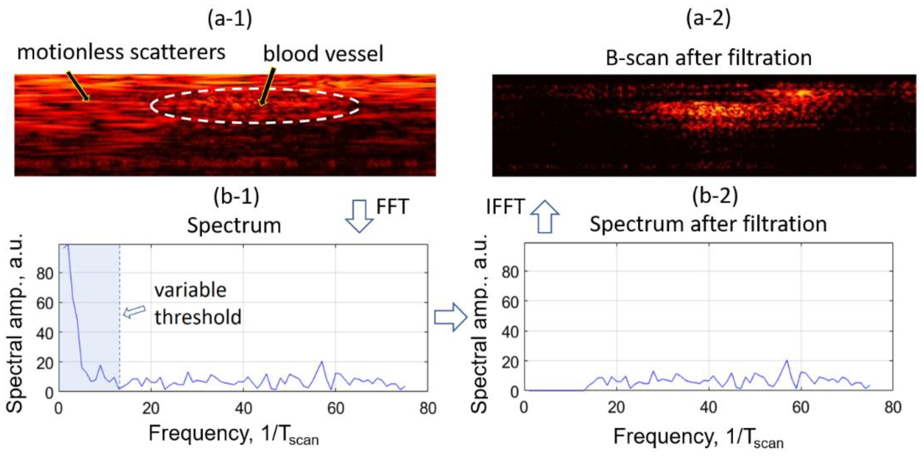
2.3. High Pass Filtering Angiography

The HP-filtering method used in this work is described in detail in [14,15]. Briefly, the filtering is applied to the array of complex-valued amplitudes of the OCT signal along the direction of slow scanning. This may be either direction along the B-scan, in the case of densely recorded B-scans such as in [14], or in the direction orthogonal to B-scans if the slow scanning axis is chosen orthogonally to the B-scans, such as in [15] and in the present study. Basically, the principle of HP-filtering in both cases is the same.

For illustration, Figure 3a shows a densely recorded B-scan in which the speckles corresponding to the motionless tissue are elongated horizontally (the degree of elongation is determined by the degree of self-overlapping of neighboring A-scans). On the contrary, in the cross section of a vessel (marked by the dash-like oval in Figure 3(a-1)), the speckles are much shorter because of the motion of blood particles. The initial B-scans (Figure 3(a-1)) are subjected to high-pass filtering along the horizontal direction of slow scanning. The spectrum found by performing Fourier transform along the slow-scanning direction for one of the horizontal profiles passing through the vessel cross section is shown in Figure 3(b-1). The frequency units $1/T_{scan}$ correspond to the inverse scanning time $T_{scan}$ along the slow scanning direction. After elimination of the low-frequency components corresponding to slowly varying signal from the “solid” tissue, the retained high-frequency components (Figure 3(b-2)) correspond to the faster-varying signals from the moving particles. After inverse Fourier transform one obtains the image in the spatial-domain, in which the signal from the “solid” tissue is essentially suppressed (Figure 3(a-2)). Prior to filtration, a vital step for operability of the method is compensation of bulk motions arising from heartbeat, breathing, etc. Those motions produce masking signals in the regions of “solid” tissue and may strongly corrupt the angiographic imaging. For translational masking motions typical of non-contact examination, the compensation is made by correcting the depth-averaged phases of adjacent A-scans (see details in [14]). For the contact mode, interframe strains caused by the contacting OCT-probe produce depth-dependent motions, for which the phase compensation should also be depth dependent and the correcting phase is estimated within a sufficiently small window with sliding depth [15]. The latter correction method will be applied in the present study.

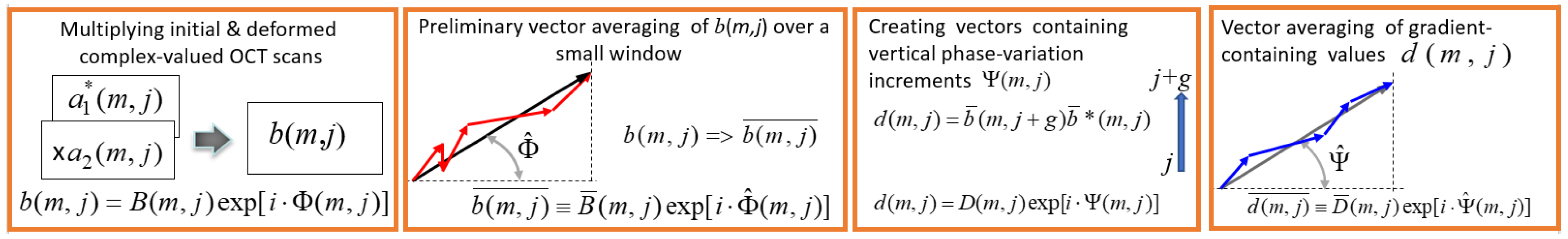
2.4. Local Strain Estimation Based Angiography (OCA-S)

As a basis for visualization of vessel cross sections, in this study, we will utilize the phase-resolved method of estimation of local strains proposed in our previous works [28,29], often used for various applications related to OCT-based elastography [21,30,31,32]. This phase-resolved method is termed “vector” because all intermediate transformations are made with complex-valued OCT-signal amplitudes $a(m,j)=A(m,j)\exp [i\cdot \phi (m,j)]$, without singling out the phase explicitly. The main stages of the vector method of local strain estimation are schematically shown in Figure 4 and comprise the following steps:

(a)

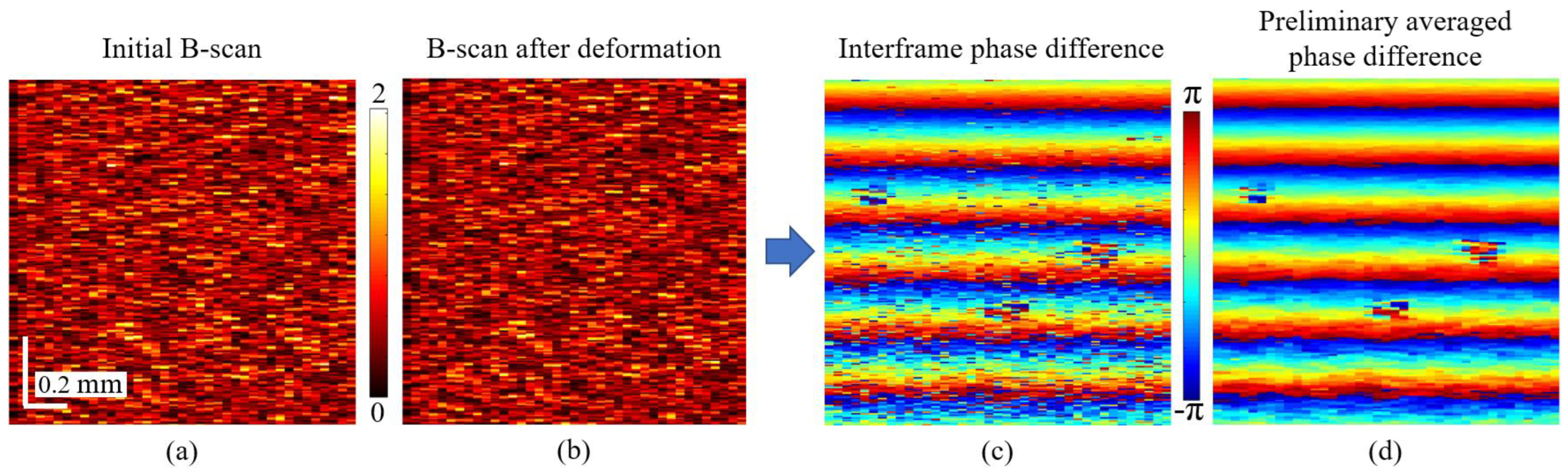
Element-by-element multiplication of the deformed B-scan and initial complex-conjugated B-scan:

$$a_2(m,j)a_1^{*}(m,j)\equiv b(m,j)=B(m,j)\exp [i\cdot \mathsf{\Phi }(m,j)]$$

(1)

where $\mathsf{\Phi }(m,j)={\phi }_2(m,j)-{\phi }_1(m,j)$ and $B(m,j)=A_2(m,j)A_1(m,j)$. The asterisk means complex conjugation. The complex-valued matrix contains information about interframe phase difference in every pixel.

(b)

For improving the signal-to noise ratio without appreciable loss in resolution, the preliminary vector averaging of $b(m,j)$ is made within a small sliding window $Mp\times Jp$ in size (usually chosen around 2 × 2 pixels):

$$\overline{b(m,j)}\equiv \overline{B}(m,j)\exp [i\cdot \widehat{\mathsf{\Phi }}(m,j)]={\displaystyle \sum _{m^{\prime }=m}^{m+Mp-1}{\displaystyle \sum _{j^{\prime }=j}^{j+Jp-1}b(m^{\prime },j^{\prime })}}$$

(2)

where vector $\overline{b(m,j)}$, found by summation of individual vectors $b(m,j)$, is characterized by the resultant amplitude $\overline{B}(m,j)$ and angle $\widehat{\mathsf{\Phi }}(m,j)$ and shown in Figure 4 (second panel).

The next step is finding the matrix containing axial phase-variation gradients:

$$d(m,j)=\overline{b}(m,j+g)\cdot \overline{b}\ast (m,j)$$

(3)

This quantity can be represented as $d(m,j)=D(m,j)\exp [i\cdot \mathsf{\Psi }(m,j)]$. The argument of this complex-valued quantity is proportional to the axial phase-variation gradient and, correspondingly, to the local axial strain. In the simplest case, the vertical step for finding this gradient is g = 1, but if there is no phase wrapping on a scale of $g>1$ pixels, a larger chosen $g>1$ may significantly improve the quality of the gradient estimation. In the case of $g>1$, the value $\arg [d(m,j)]/g$ should be used instead of $\arg [d(m,j)]$ for estimating the phase gradient.

(c)

Additional noise reduction may be obtained by vector averaging of quantity $d(m,j)=D(m,j)\exp [i\cdot \mathsf{\Psi }(m,j)]$ with a sliding window; the chosen size of this window $Mg\times Jg$ usually may be larger than for the initial averaging in Equation (2), because the phase gradient $\mathsf{\Psi }$ often exhibits slower spatial variability than the initial phase variations $\mathsf{\Phi }$.

$$\overline{d(m,j)}\equiv \overline{D}(m,j)\exp [i\cdot \widehat{\mathsf{\Psi }}(m,j)]={\displaystyle \sum _{m’=m}^{m+Mg-1}{\displaystyle \sum _{j’=j}^{j+Jg-1}d(m,j)}}$$

(4)

where, by analogy with quantity $\widehat{\mathsf{\Phi }}(m,j)$ in Equation (2), quantity $\widehat{\mathsf{\Psi }}(m,j)$ is the effective angle that is proportional to the sought averaged axial gradient of the interframe phase variation (see the last panel in Figure 4).

In view of the well-known relation between the interframe phase-variation and interframe displacement of scatterers [21],

$$u=\frac{{\lambda }_0\mathsf{\Phi }}{4\pi n}$$

(5)

The local strain $du/dz$ is proportional to the phase-variation gradient $d\mathsf{\Phi }/dz$ with the proportionality coefficient ${\lambda }_0/(4\pi n)$ (where ${\lambda }_0$ is the probing light wavelength and $n$ is the refractive index of the tissue). However, since for the discussed problem of angiographic visualization we are not interested in the absolute estimates of strains, in what follows, we will directly operate with the above defined dimensionless axial gradient $\mathsf{\Psi }$ proportional to the local strains.

It has been pointed out that, in contact mode, the compression of the examined tissue by the OCT probe causes fairly smooth strain distribution in the tissue bulk, although the displacements of scatterers may be essentially spatially inhomogeneous and have rather large supra-wavelength magnitudes. In contrast, due to the motion of blood particles, the interframe phase variation within cross sections of vessels may be arbitrary. Consequently, cross sections of the vessels can be singled out as local spots of discontinuous phase gradient against the background of fairly smooth phase gradients corresponding to the tissue around the vessels.

These local places of discontinuous phase gradient in vessel cross sections can be singled out by considering the following quantity, constructed using the above discussed axial phase-variation gradients:

$$S=\left|\mathsf{\Psi }-\widehat{\mathsf{\Psi }}\right|$$

(6)

We point out once again that quantity $\widehat{\mathsf{\Psi }}$ is the smoothed interframe phase gradient after vector averaging, defined by Equation (4), and $\mathsf{\Psi }$ is this gradient before averaging. For the signal received from “solid tissue”, the phase-variation gradient $\mathsf{\Psi }$ before averaging and the smoothed gradient $\widehat{\mathsf{\Psi }}$ after averaging are approximately equal, so the subtraction of averaged $\widehat{\mathsf{\Psi }}$ from $\mathsf{\Psi }$ is destined to eliminate the contribution of masking strain-produced displacements of scatterers in the “solid” tissue. These strain-produced displacements are much smoother than local displacement of blood particles in the vessel cross sections. Thus, the quantity $S$ for the “solid” tissue should have low magnitude. At the same time, the subtraction in Equation (6) still retains the abrupt variations in the phase-variation gradient in the vessel cross sections. Consequently, blood vessels will be seen as noisy areas on a low-signal background.

It is important to notice that noisy areas of low-level signal also correspond to random interframe phase variations. To discriminate such low-signal areas, conventionally used amplitude masking can be applied. For values $d(m,j)$ with amplitude lower than a chosen threshold, $S$ values of corresponding pixels should be disregarded.

Additionally, the $S$ values estimated for each pair of consequent B-scans can be averaged over a small window (that does not appreciably reduce lateral resolution) in the plane of B-scans, as well as in the direction of slow scanning, using a sliding window that covers the portion of self-overlapping B-scans. At all steps, the sizes of the averaging windows should be chosen as a compromise among the resolution, contrast between the vessels and “solid” tissue and overall signal-to-noise ratio. These statements are illustrated in the Section 3.

3. Results

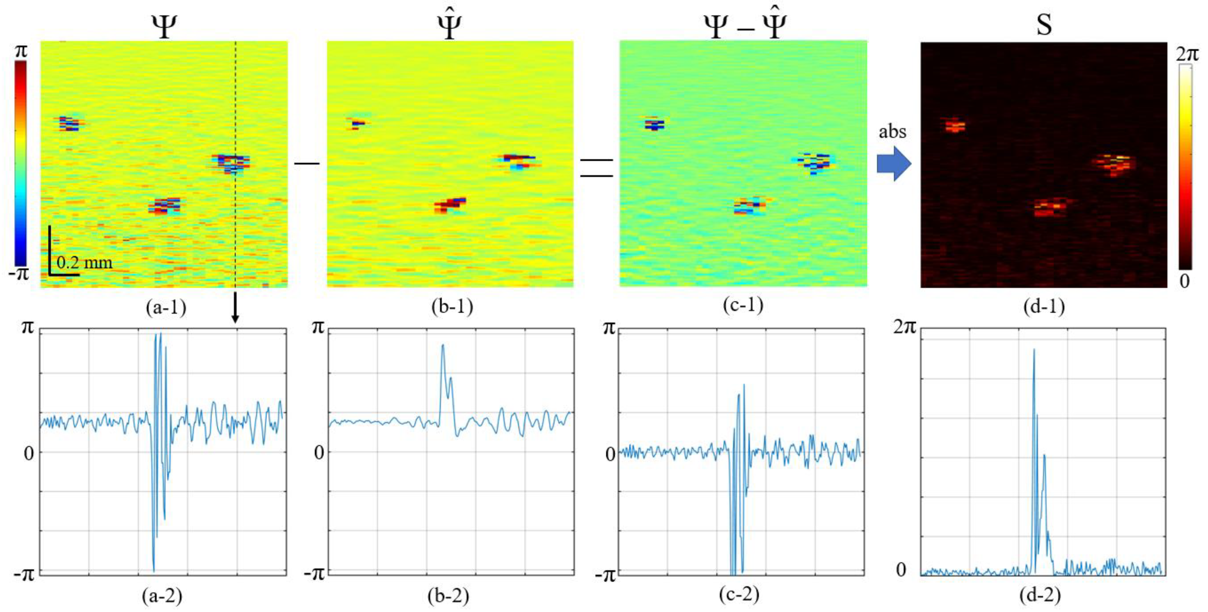
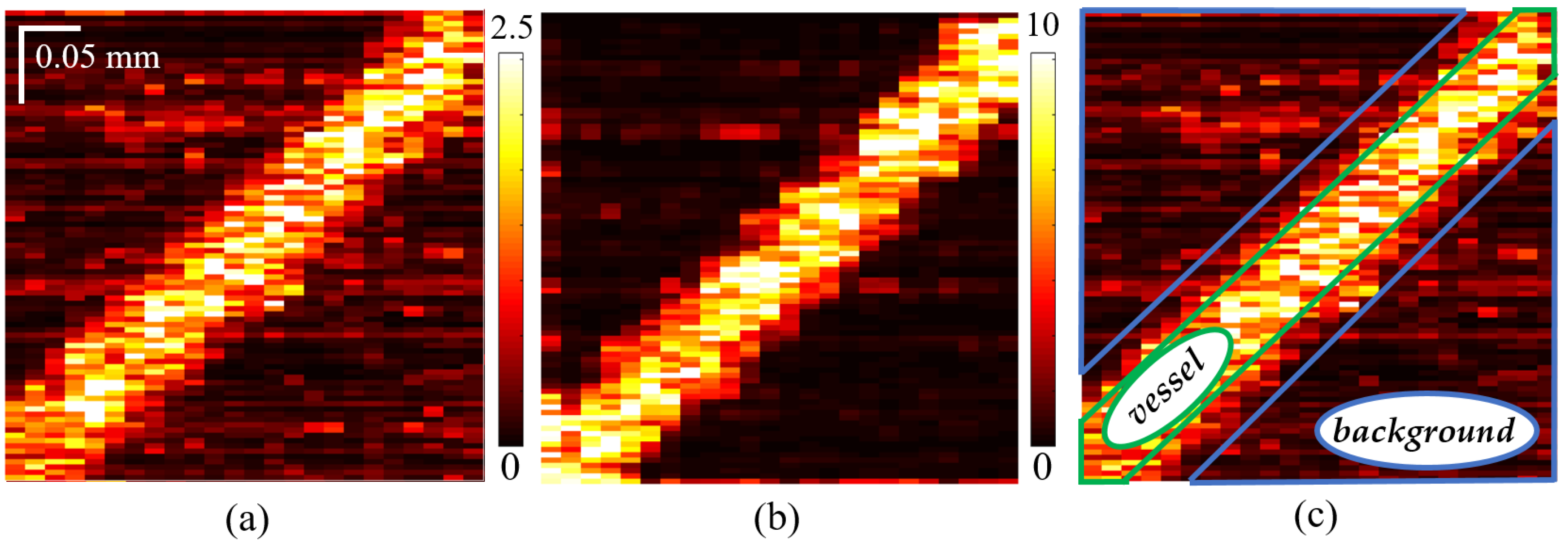
3.1. Elucidation of the Elastography-Inspired Angiography Using Simulated 2D OCA-S Images Containing Vessel Cross-Sections

For demonstration of OCA-S method (the abbreviation reflects the fact that OCA is based on the quantity $S$ given by Equation (6)), two B-scans before and after deformation were simulated (Figure 5a,b). B-scans have a size of 1000 × 640 μm and contain three vessels with diameters of 60, 70 and 80 μm, with randomly displaced blood particles inside vessel cross sections. The parameters for simulation of the OCT images were chosen to correspond to the parameters of the experimental setup described in Section 2.2. The chosen interframe strain is fairly large, s = 2 × 10⁻³. The corresponding phase difference for the frames Figure 5a,b is shown in Figure 5c. The vessels are already distinguishable in the phase-variation map, Figure 5c, as places of less regular phase variation. The magnitude of the regular displacements gradually grows with increasing depth and exceeds three wavelengths near the image bottom. The strongly increased phase noise caused by the displacement-produced decorrelation is clearly seen in the bottom part of Figure 5c.

Figure 6 illustrates the pair-wise processing of the two neighboring B-scans based on the utilization of phase-variation gradients in the initial and averaged forms and their combination given in Equation (6). Vessels are clearly visible in all the images, but subtraction of the smoothed phase gradient allows us to suppress this background signal level, and taking the absolute value of the difference is also important. As seen in Figure 6a,b, phase gradients $\mathsf{\Psi }$ have alternating sign values inside the vessels, and their averaging of several S-scans would result in zero-mean OCA signal inside the vessels. The character of the phase-gradient variations is especially clearly seen in the vertical profiles passing through one of the vessels and is shown in the lower row in Figure 6. Therefore, we take the absolute value of $S=\left|\mathsf{\Psi }-\widehat{\mathsf{\Psi }}\right|$ that is non-negative and can be efficiently averaged for several self-overlapping S-scans along the slow-scanning direction without losing the signal inside vessels.

For the vector averaging, the following parameters were used: preliminary smoothing (Equation (2)) was performed using a 2 × 2 pixel window; the axial step for gradient estimation is g = 5 pixels; phase-gradient averaging (based on Equation (4)) was performed with a window 5 × 5 pixels in size.

After these preliminary simulation-based 2D illustrations, in the next section, we will demonstrate the comparative processing of simulated 3D data using the HP-filtering and the elastography-inspired approach for obtaining conventionally used en face images.

3.2. Comparison of Simulated 3D OCA Images

For comparison of high pass filtering and the above introduced OCA-S methods, a 3D stack of B-scans with a diagonal vessel (schematically shown in Figure 1) with a diameter of 46 μm was simulated. The size of the image is 1000 × 400 × 270 μm. Erythrocytes are modeled as discrete scatterers flowing in one direction and simultaneously performing Brownian motion. (A detailed discussion of such simulations can be found in [24].)

The pressure produced by the OCT probe in contact mode of the signal acquisition usually results in the appearance of inter-frame strain. This effect was simulated as inter B-scan strains (as in the example shown in Figure 4 and Figure 5) with randomly fluctuating amplitude with a Gaussian distribution that has zero average and standard deviation STD = 2 × 10⁻³. The signal processing for the OCA-S method is the same as in Section 3.2. The additional averaging of individual S-scans in the slow scanning direction is performed over three consecutive S-scans.

As we described in Section 2.3, for realization of the HP-filtering method, a vital step is compensation of the “solid” tissue motions prior to filtering. It is performed by compensating the phase difference for the compared fragments of the two B-scans (i.e., over sufficiently small depth intervals, as described in [15]); specifically, we perform such phase comparison over a sliding window that is 4 × 4 pixels in size.

The results of the two processing methods (based on OCA-S processing and HP-filtering) are shown in Figure 7. They are represented in the conventionally used form of 2D en face images corresponding to the maximum intensity projection (MIP) of the 3D OCA data onto the horizontal plane. The advantage of using simulated data in such studies is that the actual location of vessels and the flow parameters as well as the character and magnitude of the masking motions of the tissue are exactly known and can be easily varied. Qualitatively, it is seen from Figure 7 that the OCA-S image is less corrupted by the masking tissue motions in comparison with the HP-filtering-base image. Furthermore, due to the exact knowledge of the vessel location, we can easily perform quantitative comparison of contrast for the two methods by calculating the ratio of the mean signal inside the vessel to mean signal outside the vessel:

$$\alpha =\frac{{\displaystyle \sum S_{vessel}/Are{a}_{vessel}}}{{\displaystyle \sum S_{non\_vessel}}/Are{a}_{non\_vessel}}$$

(7)

The summation of the OCA signals in Equation (7) is performed over the areas (actually, total numbers of pixels) inside and outside the vessels in the en face image, as shown in Figure 6c. The signal inside the blue triangles is considered as background and the signal inside the strip shown by the green lines is considered as blood vessel. The narrow transitional areas are not taken into account for more accurate ratio calculation. The thus-found contrast for the HP-filtering method is α = 6.3 and for OCA-S method, α = 17.2.

Thus, for the simulated 3D data, the proposed OCA-S method shows better performance. It has fewer artefacts and higher contrast between the vessel and background signal. In continuation, to verify the simulation-based results, we performed experimental tests presented in the Section 3.3.

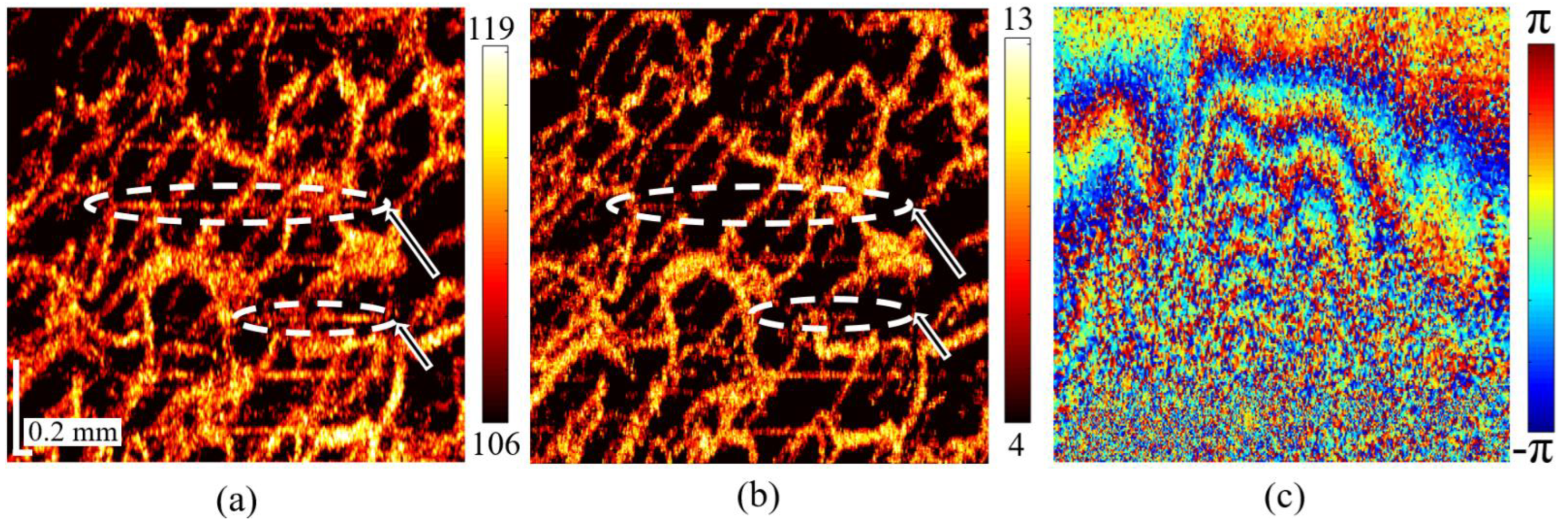
3.3. Comparison of Experimental 3D OCA Images

For the comparison of the two methods, we used a 3D image of labial mucosa from the internal lip surface of a volunteer, which consists of a set of 256 B-scans.

OCA-S signal processing is similar to that described in Section 3.2. One additional step is conventionally used amplitude thresholding, as described in Section 2.4, to eliminate the depth range with a too low-level signal. Five consequent in-depth scans were used for averaging of OCA-S scans in a slow scanning direction before obtaining MIP en face images. For high pass filtering, the bulk motion compensation was performed with a bigger sliding window (16 × 16 pixels) for better noise reduction.

For both methods, one additional processing step was performed. The angiographic signal on the final en face images was thresholded with the threshold equal to the mean value minus half of the standard deviation. All the values above the threshold were considered as vessels, with one exception: small disconnected image fragments less than several pixels in size were considered as noise and were removed for better quality visualization.

Results are presented in Figure 8 using a conventionally used logarithmic scale (in dB). Figure 8c shows the initial inter-B-scan phase-variation map corresponding to the position of the upper horizontal artefactual line marked by the dashed oval. Despite rather complex spatial structure of the strain-related masking motions, the OCA-S image in Figure 8b demonstrates that the elastography-inspired processing is able to efficiently suppress artefacts caused by such tissue motions.

4. Discussion

Based on the performed simulations and experimental results, the following main advantages of OCA-S method can be emphasized.

As is clear from the key expression (6) for the OCA-S signal, this method does not require additional procedures for compensation of masking motions arising from compression by the OCT probe (in contact mode), heartbeat, breathing, etc. The spatial distribution of those masking motions may be rather complex; in particular, the interframe displacements of scatterers may be depth-dependent. This situation is typical of contact mode OCA and does not require any special modification of the compensation procedures in comparison with depth-independent translational motions typical of non-contact examinations.

As is clear from the example shown in Figure 8c, there are fewer deformation-induced artefactual horizontal lines on the OCA-S en face image in comparison with Figure 8b for the HP-filtering method. This difference can be commented as follows: For HP-filtering (as well as for other methods based on detection of time-dependent variations in the pixels belonging to a series of consequent scans acquired for the same or nearly the same position), compensation of interframe motions is a key step. First of all, this relates to compensation of phase variations, because phase is usually more sensitive to motions of scatterers. Such compensation of relatively large-scale tissue motions is usually made by comparing the interframe phase variations with certain spatial averaging (either over the entire depth, or within a limited depth interval). On the one hand, too large averaging-window size gives incorrect phase correction for spatially non-uniform tissue motions. On the other hand, a too small averaging window may compensate for even the sought motions in the vessel cross sections and/or give too noisy and incorrect results because of “decorrelation noise” and other insufficiently averaged measurement errors. For practical usage, a compromise between these too big and too small window sizes should be chosen. However, in situations when isophase lines are dense and highly inclined (as in Figure 8a), there is no appropriate compromise between the resultant signal-to-noise ratio (SNR) and window size (strongly tilted and dense isophase lines require a smaller window, but at the same time, a small window results in low SNR). This leads to bad compensation of masking motions and, therefore, strong artefacts arise in the OCA signal when OCA scans coincide with such a place with dense and abruptly turning isophase lines.

In the proposed elastography-inspired approach, the preliminary vector averaging of the interframe phase variation is made over a rather small window size (see Equation (2)). This averaging does not yet appreciably corrupt the isophase lines (even if they are rather dense and inclined), but noticeably improves SNR.

The next step is obtaining the distribution of the axial phase-variation gradient $\mathsf{\Psi }$ via Equation (3). This phase-gradient field is spatially much smoother than the initial interframe phase-variations $\mathsf{\Phi }$ (except for the small cross sections of the sought vessels). Therefore, the gradients $\mathsf{\Psi }$ may be averaged over a larger window to obtain the averaged field $\overline{\mathsf{\Psi }}$ that is used in Equation (6) to eliminate the background strains by subtracting $\overline{\mathsf{\Psi }}$ from $\mathsf{\Psi }$. Simultaneously, this subtraction partially removes noisy fluctuations of the field $\mathsf{\Psi }$, whereas the “useful” abrupt phase-gradient variations in the vessels are not significantly affected. However, for a too big window, subtraction of the averaged gradient $\overline{\mathsf{\Psi }}$ eliminates only the smooth component of $\mathsf{\Psi }$, whereas noisy fluctuations remain unsuppressed. Thus, a compromise window size should be chosen. In this paper, we formulate only the basic principles of the elastography-inspired approach, and the above-mentioned optimizations will be specially discussed elsewhere.

One more difference between the two discussed methods can be pointed out. The HP-filtering is applied to the entire complex-valued signal, so that the constructed images of the vessels depend on the amplitude of the signal scattered by the blood particles (this usually may lead to a broader range of amplitudes in the OCA image). Unlike this, in the elastography-inspired algorithm, the local abruptly varying strains are estimated using the variability of the phase variation over the B-scan plane. Consequently, the contrast of the reconstructed vessel images does not directly depend on the amplitude of the scattered signal (certainly assuming that the noise is lower). The possibility to combine the amplitude-based and phase-based contrasts may be a promising direction for further studies.

Finally, it can be mentioned that the described elastography-based approach utilizes basically the same vector method of estimation of phase-variation gradient as is currently used for realization of OCT-based elastography. This method is very computationally efficient (especially in comparison with conventional approaches based on the least-square fitting [28]). Recently, utilization of the vector methods of strain estimation was demonstrated for on-flight visualization of strains without multicore GPU calculations [33]. Thus, the vector method can be adapted for real time OCA-visualization based on the proposed elastography-inspired principle.

5. Conclusions

The proposed elastography-inspired approach to OCT-based elastographic imaging exploits a novel variant of discrimination between the moving blood particles and the surrounding “solid” tissue which is significantly different from the earlier proposed variants of OCA. This approach utilizes the property of continuity of mechanically-produced strains in the tissue and local breaking of the strain continuity in the cross sections of the sought vessels. An important advantage of this strain-based OCA is the ease of efficient compensation of the masking tissue motions of the nearly arbitrary spatial configuration. The magnitude of these masking motions may be rather high, even of essentially supra-wavelength magnitude, although, certainly, this magnitude should not be essentially supra-pixel because, otherwise, it makes no sense to compare the consecutive OCT scans. This ability of the strain-based OCA is especially important for contact mode OCA, which is minimally invasive and, in many cases, operable on patients without the necessity of additional tissue-immobilizing devices.

Another advantage is that the elastography-inspired OCA approach uses essentially the same computationally efficient vector method for estimating local strains. In view of this, by analogy with real-time elastographic strain visualization [31], the new OCA method can enable real-time (on-flight) angiographic imaging. To further improve the quality of OCA imaging, the results of the new OCA method potentially may be combined with more conventional approaches such as HP-filtering, for which exactly the same scanning pattern can be used. Thus, the new OCA method looks very promising for enabling wider application of OCA in both laboratory studies on animals and, most importantly, for wider clinical applications on patients.

References

1. Leitgeb, R.; Placzek, F.; Rank, E.; Krainz, L.; Haindl, R.; Li, Q.; Liu, M.; Andreana, M.; Unterhuber, A.; Schmoll, T.; et al. Enhanced Medical Diagnosis for DOCTors: A Perspective of Optical Coherence Tomography. J. Biomed. Opt. 2021, 26, 100601. [Google Scholar] [CrossRef]
2. Yang, V.X.D.; Gordon, M.L.; Qi, B.; Pekar, J.; Lo, S.; Seng-Yue, E.; Mok, A.; Wilson, B.C.; Vitkin, I.A. High Speed, Wide Velocity Dynamic Range Doppler Optical Coherence Tomography (Part I): System Design, Signal Processing, and Performance. Opt. Express 2003, 11, 794–809. [Google Scholar] [CrossRef] [Green Version]
3. Leitgeb, R.A.; Schmetterer, L.; Drexler, W.; Fercher, A.F.; Zawadzki, R.J.; Bajraszewski, T. Real-Time Assessment of Retinal Blood Flow with Ultrafast Acquisition by Color Doppler Fourier Domain Optical Coherence Tomography. Opt. Express 2003, 11, 3116–3121. [Google Scholar] [CrossRef]
4. Wang, R.K.; An, L. Doppler Optical Micro-Angiography for Volumetric Imaging of Vascular Perfusion in Vivo. Opt. Express 2009, 17, 8926–8940. [Google Scholar] [CrossRef] [Green Version]
5. Kashani, A.H.; Chen, C.-L.; Gahm, J.K.; Zheng, F.; Richter, G.M.; Rosenfeld, P.J.; Shi, Y.; Wang, R.K. Optical Coherence Tomography Angiography: A Comprehensive Review of Current Methods and Clinical Applications. Prog. Retin. Eye Res. 2017, 60, 66–100. [Google Scholar] [CrossRef]
6. Mariampillai, A.; Standish, B.A.; Moriyama, E.H.; Khurana, M.; Munce, N.R.; Leung, M.K.K.; Jiang, J.; Cable, A.; Wilson, B.C.; Vitkin, I.A.; et al. Speckle Variance Detection of Microvasculature Using Swept-Source Optical Coherence Tomography. Opt. Lett. 2008, 33, 1530–1532. [Google Scholar] [CrossRef] [Green Version]
7. Mahmud, M.S.; Cadotte, D.W.; Vuong, B.; Sun, C.; Luk, T.W.H.; Mariampillai, A.; Yang, V.X.D. Review of Speckle and Phase Variance Optical Coherence Tomography to Visualize Microvascular Networks. J. Biomed. Opt. 2013, 18, 050901. [Google Scholar] [CrossRef] [Green Version]
8. Enfield, J.; Jonathan, E.; Leahy, M. In Vivo Imaging of the Microcirculation of the Volar Forearm Using Correlation Mapping Optical Coherence Tomography (CmOCT). Biomed. Opt. Express 2011, 2, 1184–1193. [Google Scholar] [CrossRef] [PubMed] [Green Version]
9. Wang, R.K.; Jacques, S.L.; Ma, Z.; Hurst, S.; Hanson, S.R.; Gruber, A. Three Dimensional Optical Angiography. Opt. Express 2007, 15, 4083–4097. [Google Scholar] [CrossRef]
10. Makita, S.; Hong, Y.; Yamanari, M.; Yatagai, T.; Yasuno, Y. Optical Coherence Angiography. Opt. Express 2006, 14, 7821–7840. [Google Scholar] [CrossRef] [Green Version]
11. Jia, Y.; Tan, O.; Tokayer, J.; Potsaid, B.; Wang, Y.; Liu, J.J.; Kraus, M.F.; Subhash, H.; Fujimoto, J.G.; Hornegger, J.; et al. Split-Spectrum Amplitude-Decorrelation Angiography with Optical Coherence Tomography. Opt. Express 2012, 20, 4710–4725. [Google Scholar] [CrossRef] [Green Version]
12. Postnov, D.D.; Tang, J.; Erdener, S.E.; Kılıç, K.; Boas, D.A. Dynamic Light Scattering Imaging. Sci. Adv. 2020, 6, eabc4628. [Google Scholar] [CrossRef]
13. Tang, J.; Erdener, S.E.; Sunil, S.; Boas, D.A. Normalized Field Autocorrelation Function-Based Optical Coherence Tomography Three-Dimensional Angiography. J. Biomed. Opt. 2019, 24, 036005. [Google Scholar] [CrossRef] [Green Version]
14. Matveev, L.A.; Zaitsev, V.Y.; Gelikonov, G.V.; Matveyev, A.L.; Moiseev, A.A.; Ksenofontov, S.Y.; Gelikonov, V.M.; Sirotkina, M.A.; Gladkova, N.D.; Demidov, V.; et al. Hybrid M-Mode-like OCT Imaging of Three-Dimensional Microvasculature in Vivo Using Reference-Free Processing of Complex Valued B-Scans. Opt. Lett. 2015, 40, 1472–1475. [Google Scholar] [CrossRef]
15. Moiseev, A.; Ksenofontov, S.; Sirotkina, M.; Kiseleva, E.; Gorozhantseva, M.; Shakhova, N.; Matveev, L.; Zaitsev, V.; Matveyev, A.; Zagaynova, E.; et al. Optical Coherence Tomography-Based Angiography Device with Real-Time Angiography B-Scans Visualization and Hand-Held Probe for Everyday Clinical Use. J. Biophotonics 2018, 11, e201700292. [Google Scholar] [CrossRef]
16. Demidov, V.; Matveev, L.A.; Demidova, O.; Matveyev, A.L.; Zaitsev, V.Y.; Flueraru, C.; Vitkin, I.A. Analysis of Low-Scattering Regions in Optical Coherence Tomography: Applications to Neurography and Lymphangiography. Biomed. Opt. Express 2019, 10, 4207–4219. [Google Scholar] [CrossRef]
17. Sirotkina, M.A.; Moiseev, A.A.; Matveev, L.A.; Zaitsev, V.Y.; Elagin, V.V.; Kuznetsov, S.S.; Gelikonov, G.V.; Ksenofontov, S.Y.; Zagaynova, E.V.; Feldchtein, F.I.; et al. Accurate Early Prediction of Tumour Response to PDT Using Optical Coherence Angiography. Sci. Rep. 2019, 9, 6492. [Google Scholar] [CrossRef]
18. Matveev, L.; Kiseleva, E.; Baleev, M.; Moiseev, A.; Ryabkov, M.; Potapov, A.; Bederina, E.; Sirotkina, M.; Shalin, V.; Smirnov, I.; et al. Optical Coherence Tomography Angiography and Attenuation Imaging for Label-Free Observation of Functional Changes in the Intestine after Sympathectomy: A Pilot Study. Photonics 2022, 9, 304. [Google Scholar] [CrossRef]
19. Maslennikova, A.V.; Sirotkina, M.A.; Moiseev, A.A.; Finagina, E.S.; Ksenofontov, S.Y.; Gelikonov, G.V.; Matveev, L.A.; Kiseleva, E.B.; Zaitsev, V.Y.; Zagaynova, E.V.; et al. In-Vivo Longitudinal Imaging of Microvascular Changes in Irradiated Oral Mucosa of Radiotherapy Cancer Patients Using Optical Coherence Tomography. Sci. Rep. 2017, 7, 16505. [Google Scholar] [CrossRef]
20. Gubarkova, E.V.; Feldchtein, F.I.; Zagaynova, E.V.; Gamayunov, S.V.; Sirotkina, M.A.; Sedova, E.S.; Kuznetsov, S.S.; Moiseev, A.A.; Matveev, L.A.; Zaitsev, V.Y.; et al. Optical Coherence Angiography for Pre-Treatment Assessment and Treatment Monitoring Following Photodynamic Therapy: A Basal Cell Carcinoma Patient Study. Sci. Rep. 2019, 9, 18670. [Google Scholar] [CrossRef]
21. Zaitsev, V.Y.; Matveyev, A.L.; Matveev, L.A.; Sovetsky, A.A.; Hepburn, M.S.; Mowla, A.; Kennedy, B.F. Strain and Elasticity Imaging in Compression Optical Coherence Elastography: The Two-decade Perspective and Recent Advances. J. Biophotonics 2021, 14, e202000257. [Google Scholar] [CrossRef]
22. Yao, G.; Wang, L.V. Monte Carlo Simulation of an Optical Coherence Tomography Signal in Homogeneous Turbid Media. Phys. Med. Biol. 1999, 44, 2307–2320. [Google Scholar] [CrossRef] [PubMed]
23. Kirillin, M.; Meglinski, I.; Kuzmin, V.; Sergeeva, E.; Myllylä, R. Simulation of Optical Coherence Tomography Images by Monte Carlo Modeling Based on Polarization Vector Approach. Opt. Express 2010, 18, 21714–21724. [Google Scholar] [CrossRef]
24. Doronin, A.; Meglinski, I. Online Object Oriented Monte Carlo Computational Tool for the Needs of Biomedical Optics. Biomed. Opt. Express 2011, 2, 2461–2469. [Google Scholar] [CrossRef] [Green Version]
25. Zaitsev, V.Y.; Matveev, L.A.; Matveyev, A.L.; Gelikonov, G.V.; Gelikonov, V.M. A Model for Simulating Speckle-Pattern Evolution Based on Close to Reality Procedures Used in Spectral-Domain OCT. Laser Phys. Lett. 2014, 11, 105601. [Google Scholar] [CrossRef] [Green Version]
26. Zykov, A.; Matveyev, A.; Matveev, L.; Sovetsky, A.; Zaitsev, V. Flexible Computationally Efficient Platform for Simulating Scan Formation in Optical Coherence Tomography with Accounting for Arbitrary Motions of Scatterers. J. Biomed. Photon. Eng. 2021, 7, 010304. [Google Scholar] [CrossRef]
27. Almasian, M.; van Leeuwen, T.G.; Faber, D.J. OCT Amplitude and Speckle Statistics of Discrete Random Media. Sci. Rep. 2017, 7, 14873. [Google Scholar] [CrossRef] [Green Version]
28. Zaitsev, V.Y.; Matveyev, A.L.; Matveev, L.A.; Gelikonov, G.V.; Sovetsky, A.A.; Vitkin, A. Optimized Phase Gradient Measurements and Phase-Amplitude Interplay in Optical Coherence Elastography. J. Biomed. Opt 2016, 21, 116005. [Google Scholar] [CrossRef]
29. Matveyev, A.L.; Matveev, L.A.; Sovetsky, A.A.; Gelikonov, G.V.; Moiseev, A.A.; Zaitsev, V.Y. Vector Method for Strain Estimation in Phase-Sensitive Optical Coherence Elastography. Laser Phys. Lett. 2018, 15, 065603. [Google Scholar] [CrossRef]
30. Li, J.; Pijewska, E.; Fang, Q.; Szkulmowski, M.; Kennedy, B.F. Analysis of Strain Estimation Methods in Phase-Sensitive Compression Optical Coherence Elastography. Biomed. Opt. Express 2022, 13, 2224. [Google Scholar] [CrossRef]
31. Kling, S.; Khodadadi, H.; Goksel, O. Optical Coherence Elastography-Based Corneal Strain Imaging during Low-Amplitude Intraocular Pressure Modulation. Front. Bioeng. Biotechnol. 2020, 7, 453. [Google Scholar] [CrossRef] [PubMed] [Green Version]
32. Kling, S. Optical Coherence Elastography by Ambient Pressure Modulation for High-Resolution Strain Mapping Applied to Patterned Cross-Linking. J. R. Soc. Interface 2020, 17, 20190786. [Google Scholar] [CrossRef]
33. Zaitsev, V.Y.; Ksenofontov, S.Y.; Sovetsky, A.A.; Matveyev, A.L.; Matveev, L.A.; Zykov, A.A.; Gelikonov, G.V. Real-Time Strain and Elasticity Imaging in Phase-Sensitive Optical Coherence Elastography Using a Computationally Efficient Realization of the Vector Method. Photonics 2021, 8, 527. [Google Scholar] [CrossRef]
Figure 1. Schematic of the 2D and 3D images containing scatterers used in the simulations. (a) 2D cross section containing three blood vessels (red colored dots) surrounded by “solid” tissue (yellow); (b) 3D volume in which the diagonal cylinder represents the vessel filled with moving blood particles. The rest of the volume for 3D is also filled by scatterers imitating the “solid” tissue, but these scatterers are not shown. Scatterers of the “solid” tissue have the same concentration and scattering strength as in the vessel for both 2D and 3D datasets.
Photonics 09 00401 g001
Figure 2. Illustration of the scanning of biological tissue along fast (a) and slow (b) scanning directions.
Photonics 09 00401 g002
Figure 3. Schematic of the high pass filtering method. Fourier transform of B-scan is taken along a slow scanning direction (horizontal in the figure). Due to much higher speckle pattern variability inside the vessels (see panel (a-1)), they contribute to the high-frequencies range in the spectrum, whereas motionless tissue corresponds to low frequencies that can be filtered out (compare panels (b-1) before filtering and (b-2) after filtering). Therefore, high-pass filtering suppresses the “solid tissue” and makes vessels visible in the spatial-domain image constructed by inverse Fourier transform (a-2).
Photonics 09 00401 g003
Figure 4. Schematic of the vector method for axial phase gradient evaluation. All intermediate calculations are performed with complex-valued signals considered as vectors in the complex plane. Phase gradient is extracted at the last processing step.
Photonics 09 00401 g004
Figure 5. Simulated OCT images: (a) Structural B-scan before deformation; (b) B-scan after tissue deformation. B-scans are very similar and it is impossible to identify the vessels using only structural images. The pixel-to-pixel interframe phase difference between B-scans is shown in (c), and (d) represents this difference in a less noisy form due to vector averaging over a small window 2 × 2 pixels. The scale bar is 0.2 mm.
Photonics 09 00401 g005
Figure 6. Illustration of OCA-S signal processing based on Equation (6). Upper row—2D images; lower row—1D profiles, corresponding to A-scan that passes through one of the vessels as marked by the dashed line on a panel (a-1). Ψ —axial phase gradient, Ψ ^ —vector averaged phase gradient. Both quantities have a non-zero average value proportional to the interframe strain, which is removed by subtraction of Ψ and Ψ ^ (panel (c-1)). It is necessary to take the absolute value (shown in panel (d-1)) for further averaging for several overlapping S-scans, because, otherwise, averaging of alternating sign values inside the vessels results in a signal decrease down to zero mean value. In the final S image, there are three clearly visible blood vessels that appear as noise regions on a low signal background. The scale bar is 0.2 mm.
Photonics 09 00401 g006
Figure 7. Comparison of high pass filtration (a) and OCA-S (b) methods for simulated data. OCA-S en face image has lower background signal and has fewer strain-induced artefacts. Panel (c) illustrates areas used for calculation of ratio of mean signal inside the vessel (green figure) to mean background signal (blue triangles). The scale bar is 0.05 mm.
Photonics 09 00401 g007
Figure 8. Comparison of high pass filtration (a) and OCA-S (b) methods for experimental data. The experimental results are presented as en face images using logarithmic scale. The OCA-S image has fewer artefacts, which are indicated by white dashed ellipses. The interframe phase difference corresponding to higher ellipse is shown on panel (c). The scale bar is 0.2 mm.
Photonics 09 00401 g008
Publisher’s Note: MDPI stays neutral with regard to jurisdictional claims in published maps and institutional affiliations.