Abstract
We show that there is an intrinsic link between the use of Walsh aberration modes in adaptive optics (AO) and the mathematics of lattices. The discrete and binary nature of these modes means that there are infinite combinations of Walsh mode coefficients that can optimally correct the same aberration. Finding such a correction is hence a poorly conditioned optimisation problem that can be difficult to solve. This can be mitigated by confining the AO correction space defined in Walsh mode coefficients to the fundamental Voronoi cell of a lattice. By restricting the correction space in this way, one can ensure there is only one set of Walsh coefficients that corresponds to the optimum correction aberration. This property is used to enable the design of efficient estimation algorithms to solve the inverse problem of finding correction aberrations from a sequence of measurements in a wavefront sensorless AO system. The benefit of this approach is illustrated using a neural-network-based estimator.
1. Introduction
Many adaptive optics (AO) methods have been developed to compensate phase aberrations in a range of applications including astronomy, ophthalmology and microscopy [1,2,3]. All AO systems are limited, in some way, by the capabilities of the adaptive element, typically a deformable mirror (DM) or a spatial light modulator (SLM), that corrects the aberrations. One such limitation is in the range of phase functions that the element can correct. The correction space of an AO element is defined by the range of phase functions that can be imparted by the device. For a pixelated AO device, such as a SLM or segmented DM, the correction space is defined by the set of accessible pixel states, which could be represented by the set of phase values for each pixel.
In many AO systems, it is preferable to design the system around a set of orthogonal modes for representation and control of the wavefront, rather than localized wavefront modulations. For example, wavefont-sensorless AO systems usually use a modal basis [4,5]. This method involves the sequential application of predetermined bias aberrations, the acquisition of a set of measurements of an appropriate quality metric, and then estimation of the required correction aberration. The conventional approach to sensorless AO is to use knowledge of the forward problem—that is how the quality metric is affected by input aberrations—to inform the design of an efficient estimation scheme that, in effect, solves the inverse problem of finding the optimal correction aberrations from the set of metric measurements. Such estimation can be performed using optimisation algorithms or neural networks (NN) to solve the inverse problem [6,7].
It is known that control using modes defined across the whole pupil provides stronger modulation of the optimisation metric than individual pixels or subregions of the pupil [5]. Such whole-pupil modulation hence provides more robust operation, particularly in low-light level imaging scenarios when the signal-to-noise ratio (SNR) is low. For such pixel-based sensorless AO systems, Walsh modes are an appropriate choice. Walsh modes are a set of orthogonal functions that represent phase patterns across a pixelated pupil, where the number of pixels is equal to a power of 2 [8,9]. Each Walsh mode consists of an equal number of pixels taking each of the binary values or . For the different modes, a different combination of pixels takes the positive and negative values.
The binary nature of Walsh modes means that the range of each mode that must be searched to find the optimum correction is finite. This contrasts with other modal bases built upon continuous functions, such as Zernike polynomials, which would have unbounded range (albeit limited by the stroke of the adaptive correction element).
However, care needs to be taken when considering combinations of Walsh modes, as multiple combinations of modes can have the same effect on the system. This means that there are multiple potential solutions to the inverse problem of finding the optimal set of Walsh mode coefficients that optimise aberration correction. These multiple solutions can cause complications in defining an estimator to solve the inverse problem. Solving the inverse problem would be considerably simplified if we could ensure that there was only one optimal solution in the search space.
We show that there are properties of the Walsh modes that link the operation of these sensorless AO systems to the mathematics of lattices [10]. We discuss how these mathematical properties can aid the design of aberration estimation algorithms by constraining the search space. Specifically, we show heuristically that through understanding of the lattice geometry, we can define a unique finite search space, in terms of combinations of Walsh mode coefficients, that contains a single optimum correction. This permits the implementation of an efficient NN-based optimisation scheme that can measure and correct any combination of N Walsh modes of any coefficient value using only metric measurements. We show that a simple NN can be trained to solve the inverse problem if the search space is constrained using the lattice model, whereas the correct combination of Walsh mode coefficients cannot reliably be found for a nonconstrained search space.
2. Optical System Model
For the purposes of modelling, we considered the simple sensorless adaptive optics system shown in Figure 1. Such a model has been extensively used for analysis of such sensorless systems [11,12], as the principle of operation is readily extendable to similar optical systems, including applications in laser material processing, free-space communications, and laser scanning microscopy.
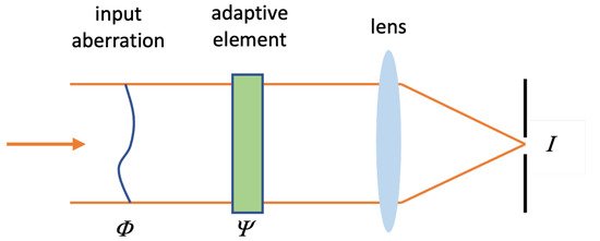
Figure 1.
Optical system used for modelling. The input wavefront contains a phase aberration , which passes through a correction device imparting an additional phase . The beam is focussed onto a vanishingly small pinhole detector on the optical axis that admits the intensity I.
The input beam to the system is collimated and has uniform amplitude. The input phase aberration is and the phase is added by the adaptive element (AE), which could be a pixelated SLM or a segmented DM. These are both considered to be added at the pupil P, which is taken to have unit radius; is the normalised coordinate vector in the pupil. The lens performs a Fourier transform of the pupil field to provide a focal field. A vanishingly small pinhole detector is placed on axis at the centre of the focus and detects a signal I that corresponds to the on-axis intensity at the focus. This is equivalent to the power of the zero-frequency component of the Fourier transform, which is equivalent to the squared modulus of the mean value of the pupil field. Mathematically, this can be expressed as
where the maximum, aberration-free signal is normalised to 1.
3. Representation of Aberrations as Walsh Modes
For simplicity, let us assume so that all aberrations can be represented within . Let us also assume that the adaptive element is a pixelated device, where each of the N pixels can introduce a piston phase. The phase introduced by the adaptive element could be expressed as
where are the phase influence functions of each pixel, which have value 1 within the pixel area and 0 elsewhere; are the coefficients of these influence functions, which correspond to the pixel phase value. Alternatively, we could represent the AE phase as
where are functions that take binary values of or in each pixel region, such that the lth pixel takes on the lth value of the kth Walsh function of length N, [8]. are the coefficients of these functions . For a given sequence length , where is an integer, there are N orthogonal Walsh functions, each of which consists of elements of value or , except for the first function that consists entirely of 1 s (see examples in Figure 2). We follow the convention that the Walsh function index starts at . From the above relationships, it is clear that each pixel phase can be represented as
or alternatively in matrix–vector format as
where is a vector of length N that contains the phase value of each pixel, is a vector of length N that contains the coefficient of each Walsh function and is an Walsh–Hadamard matrix consisting of values [13,14]. The rows of this matrix correspond to each of the Walsh functions. The matrix provides the mapping between the Walsh coefficients and the pixel values. For Hadamard matrices, , where is the identity matrix of size N [13,14]. Hence, we can invert Equation (5) as

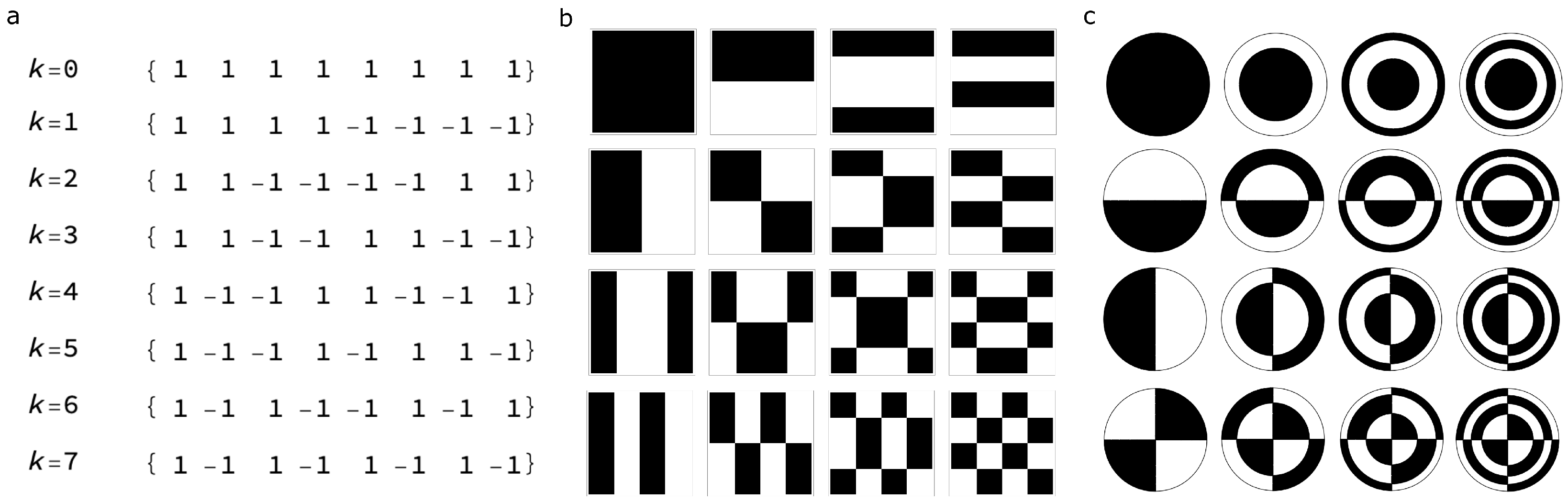
Figure 2.
Illustrations of Walsh modes. (a) The Walsh functions shown in numerical form. (b) The Walsh modes shown as aberration basis modes over a square aperture. (c) The polar Walsh modes, equivalent to shown as aberration basis modes over a circular aperture. In both (b) and (c), index for the first mode is in the top left, and k increments in row-major order to in the bottom right.
Note that for a set of Walsh functions to be defined, we require , where is an integer. We assume throughout this paper therefore that . However, Hadamard matrices also exist for , where is an integer [13,14]. For simplicity, these other matrices will not be considered in this current analysis.
4. Lattice Symmetry of Aberration States
We can define the aberration state fully as the vector of pixel values . Thus, we can consider that a point at position in the N-dimensional space of pixel values is equivalent to an aberration state where any coefficient is replaced by , where q is an arbitrary integer. This reveals a repetitive structure in each coordinate of the N-dimensional space that results in a lattice type symmetry. Hence, in this space, there is an infinite number of points that represent a given aberration state and these points are arranged in a transformed integer lattice that is scaled by a factor of and offset by the pixel value along each dimension. Furthermore, the lattice structure is based around a fundamental unit that is an N-dimensional cube of side length ; this fundamental unit is known as a Voronoi cell [10].
The matrix–vector operation of Equation (6) can now be interpreted as a rotation (as is an orthogonal matrix) and scaling by of the vector to give the Walsh coefficient vector . The lattice symmetry is hence maintained in a rotated and scaled form when the state is described by . When represented by the vector , any Walsh function consists of equal magnitude amounts ( or ) of each pixel value, so the vector must be directed along certain body diagonals of the cubic Voronoi cell. After transformation, these body diagonals lie along the axes of the vector space containing . This lattice symmetry will be used for derivations later in this article.
5. Effects of Pixels and Modes on Signal Modulation
Let us assume that each pixel of the AE has equal area (the pixels should have equal area if the amplitude profile at the pupil is uniform. For nonuniform illumination, the pixel area should be varied to provide the same total power in each pixel (e.g., the pixels could be large near the edge of the pupil for a Gaussian illumination profile.) No constraint is placed here on the position or shape of the pixels.), so that the integration used in Equation (1) can be replaced by a summation, assuming here that :
If the arbitrarily chosen lth pixel is varied and all other pixel values have the same value (here arbitrarily set to zero), then
where the modulation depth . For all other Walsh functions other than , the signal is also cyclic as a function of :
where the modulation depth has the maximum possible value of 1 and the period in terms of is . The effects of single pixel and modal variations are shown in Figure 3.
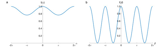
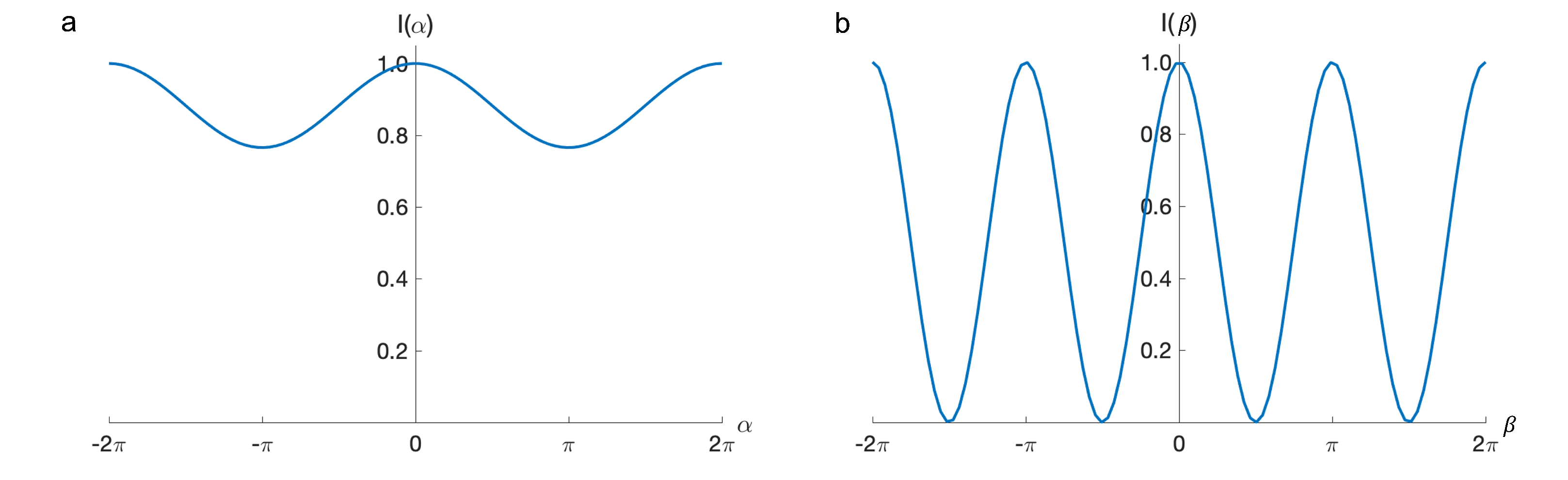
Figure 3.
(a) Variation of signal for a 16-pixel system with a single pixel modulation showing low modulation depth and period . (b) variation of a Walsh mode in the same system showing full modulation and period .
If a combination of Walsh modes is present with small coefficients, we can use a Maclaurin expansion of the exponential in Equation (7) to give
The term in the final bracket is equal to zero except for when , in which case it has value 1. The orthogonality property of the Walsh functions means that in the second term is equivalent to the Kronecker delta function . Hence, the signal is approximately
This is equivalent to the well-known approximation of the Strehl ratio as , where is the root mean square value of the aberration, which in this case is equal to .
6. Defining a Well-Corrected System
If we define our system to be “well-corrected” when the root-mean-square (rms) phase error is below a chosen value, such that , then the system will be well-corrected when . We can also express the second term in Equation (11) as a length vector , which is equivalent to with the piston coefficient removed, as
Our condition for being well-corrected is hence equivalent to requiring that . Interpreted geometrically, this means that any point within an -dimensional spherical volume of radius centred on the point where will be considered well-corrected.
In practice, the total aberration in a system will be the sum of the input aberration and that introduced by the AE, that is . The values of discussed here consolidate these two sources of aberrations to represent the residual aberrations, such that we seek a perfect correction for which . We will also assume for this analysis that the input aberration consists entirely of modes that can be corrected by the AE.
7. Vector Space Representation of Well-Corrected States
The signal variation as a function of pixel values was given in Equation (7) and can be expressed alternatively as
where . From this, we find the value can only be obtained if for all l. We derive this result by considering the phasor sum of each of the terms in the final modulus expression: the maximum signal is only obtained when all of the exponential terms in the summation are real.
In a more general case where all pixels are offset by a mean pixel phase value c rather than the first pixel phase value, we could state that only if each element of the vector has a value where n is an arbitrary integer. We can also express the signal explicitly as ; this is a function of the vector , which describes a point in an N-dimensional space. In this way, we can see that has maximum value 1 at the origin of this space when c is zero. Furthermore, we see that there is an infinite number of points in this space at which . For example, on each of the axes, there are points where that are equally spaced at steps of . Varying the value of c is equivalent to adding a constant phase to every pixel (or equivalent to adding the piston mode to the whole pupil) and thus has no effect on the signal. We deduce therefore that there are infinite lines of parallel to the vector . As the value of c has no effect on the signal, we can set this arbitrarily to zero without affecting further analysis. This is equivalent to removing the piston mode. It is also equivalent to taking the dimensional subspace including the origin in an orientation orthogonal to the direction . The position of the maxima in this slice would be equivalent to the positions of a scaled version of the integer lattice , as explained in Section 3, projected along the direction . An illustration is provided in Figure 4.
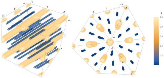
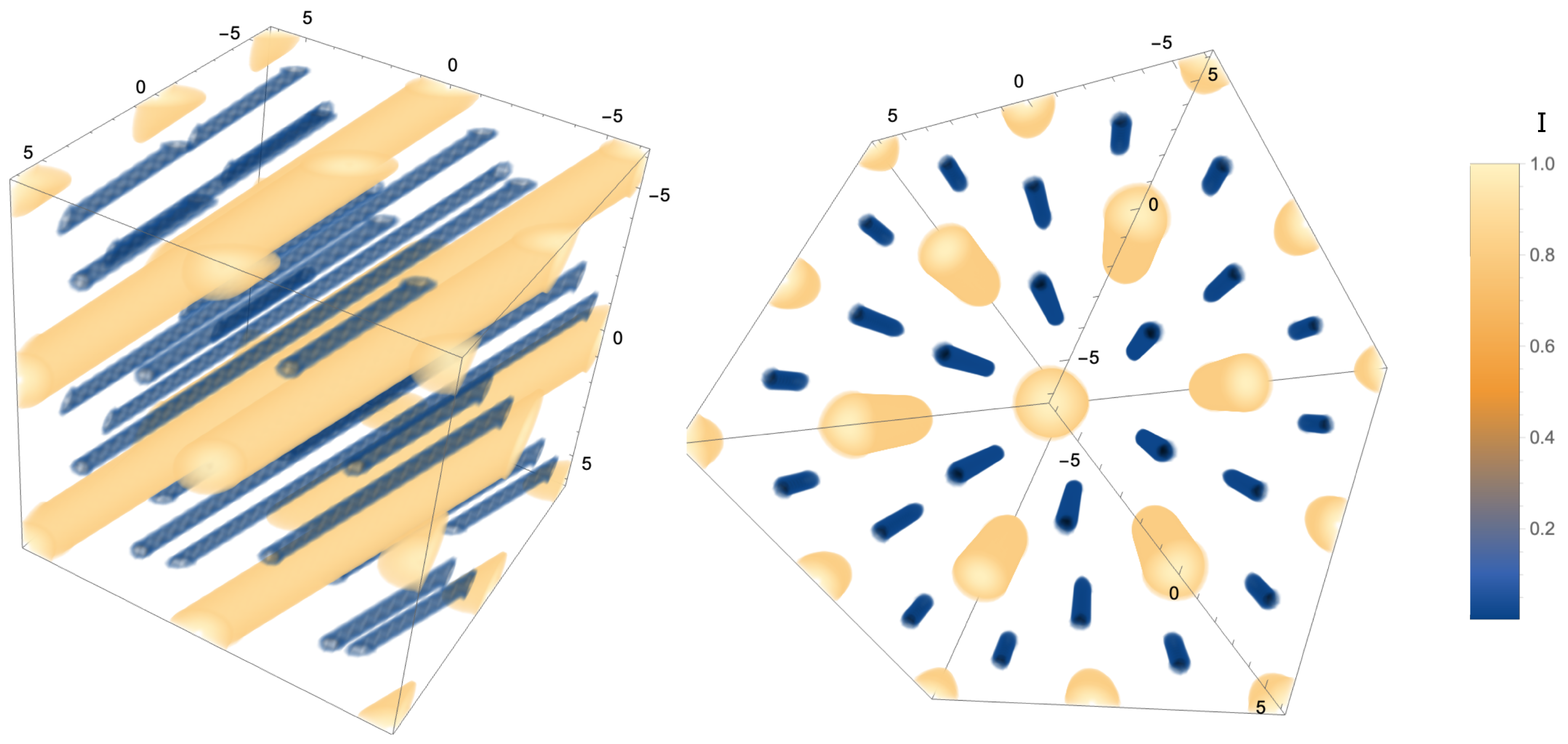
Figure 4.
Illustration of the lattice geometry for intensity variation with pixel phase value. As it is not possible to represent higher order systems in a three-dimensional rendering, the example shown is for a three-pixel system. While this system does not use Walsh modes, it shows the same phenomena of piston invariance and lattice-like behaviour. The axes represent each of the pixel phase values in radians. The same volume rendering is shown from two different angles. The visible contours are set at (blue) and (orange) to show the positions of the zeros and the maxima, respectively. The function I is invariant with the piston mode, hence the elongation of the contours along the direction . The lattice like structure of the function is apparent, in this case in the form of the hexagonal lattice. This shows that there are many different combinations of aberration mode coefficients that provide a similar well-corrected state. Analogous behaviour is found in higher dimensions for the Walsh-mode-based systems.
8. Lattice Representation of States after Removal of Piston
The removal of the piston mode is equivalent to the removal of the first row of the matrix to create the reduced matrix and removing the corresponding element of to obtain a reduced vector so that
As row–column products represent dot products between Walsh vectors, the following relationship is valid: , so Equation (14) can be inverted as
We can interpret Equation (15) as a transformation from an N-dimensional vector of pixel values to an -dimensional vector of Walsh modal coefficients .
The matrix is, however, a redundant representation, as the column space has dimension greater than its rank. This is rectified by removal of any one of the columns to create the matrix ; we choose arbitrarily to remove the first column. In order to maintain the form of Equation (15), we remove the first element of the vector to produce a new vector . From a practical perspective, this means that the pixel value is a dependent parameter determined by the other pixel values because of removal of the piston mode.
The operation performed by matrix is to map the vector to the corresponding vector . Similarly, the operation of would be to transform (project) the positions of the maxima of , which were located on lines passing through a scaled integer lattice (as illustrated in Figure 4), to another lattice in the -dimensional space spanned by .
We can determine the properties of this new lattice by considering its Gram matrix, which is the matrix of the inner products between its lattice vectors [10]. The Gram matrix is hence given by
where the factor of has been chosen so that the basis vectors are equivalent to Walsh functions with normalised vector magnitudes. is equivalent to the Gram matrix of the so-called lattice [10], which is an -dimensional analogue of the body centred cubic (BCC) lattice in three dimensions. It follows that the maxima in the -dimensional space spanned by must be located at the lattice points of a scaled lattice.
Understanding the symmetries of this lattice thus provides an understanding of the symmetries of the function . For example, the response of the signal around each lattice point should be identical. In other words, for all m, where represents an arbitrary lattice point. As there is an infinite number of lattice points, there is an infinite combination of the Walsh coefficients that can provide the optimal correction. Furthermore, correction to a precision of can be achieved by finding a setting for the adaptive correction device that places within a sphere of radius centred upon any of the lattice points.
9. Fundamental Correction Space
The lattice model allows us to define a fundamental correction space—that is, the range of we must search to find an optimal correction. This fundamental correction space is smaller than the correction space covered by all pixel values in the range 0 to radians. The lattice symmetry of the function indicates that we need only search the Voronoi cell of the lattice in order to cover all possible states. Therefore, the search space is the Voronoi cell of the scaled lattice, whose properties are known [10]. The position of the cell’s vertices can be readily calculated. For example, the Voronoi cell of the (or BCC) lattice is a truncated octahedron; this would be the Voronoi cell for a pixel system and is illustrated in Figure 5.

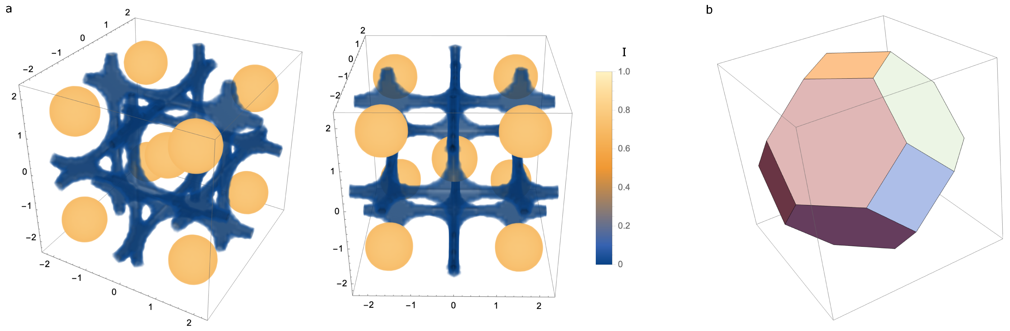
Figure 5.
(a) Illustration of the lattice geometry for the fundamental correction space of a four-pixel system, which corresponds to three Walsh modes after neglecting the piston mode. The axes represent each of the Walsh coefficient values in radians. The same volume rendering is shown from two different angles. The visible contours are set at (blue) and (orange) to show the positions of the zeros and the maxima, respectively. The BCC lattice geometry is apparent. (b) The Voronoi cell for the (or BCC) lattice, a truncated octahedron, is shown within an encompassing cube of side length radians.
Using the symmetries of the Voronoi cell, further general properties of this fundamental correction space can be derived. Moving along any of the axes from a lattice point at which , we encounter another lattice point at a distance (noting that this corresponds to the variation of a single Walsh function, the pixel values of which will be for this value of b; see Equation (9)). Therefore, the halfway point between lattice points along the axis is at a distance . Hence, the distance between two faces of the Voronoi cell along such an axis is . By looking solely along the axes, one might assume that the search space is an -dimensional cube of side length , which would have a volume of . However, the Voronoi cell’s volume is given by
which is a factor smaller than the encompassing hypercube [10]. Hence, for large numbers of pixels, the search space is considerably smaller than might be assumed if considering the pixel phases directly.
10. Implications of the Lattice Structure for Sensorless AO
We have shown that searching the Voronoi cell of the lattice is sufficient to find the optimal correction in the whole Walsh coefficient space of the adaptive element. The lattice structure also means that this same cell repeats over the whole space. Consequently, if the aberration in the system can be accurately represented by a finite number of Walsh modes, then the necessary search space is finite. This contrasts with an aberration represented by a finite number of continuous modes, such as Zernike polynomials, where the search space would have to be infinite in extent to cover all possible coefficient values.
In modal sensorless AO correction schemes, a sequence of predetermined bias aberrations for fixed set of correction modes is applied to the adaptive element and the corresponding signal values are recorded. From this set of measurements, the correction aberration is estimated using an appropriately chosen optimisation algorithm. When using continuous modes, such estimation can provide accurate correction for aberrations over a limited magnitude range but usually provides poor estimation outside this range. Using Walsh modes, however, the finite search space within one Voronoi cell of the lattice structure for a fixed set of modes means that it is possible to design a correction scheme that is accurate across all possible aberrations within the Walsh mode set. For the continuous modes, the bias aberrations span a finite range, such as in the typical configuration for sensorless AO of having equal magnitude positive and negative biases for each mode. However, the same configuration for Walsh modes in effect spans an infinite range, as the bias positions are also repeated in the lattice structure across the whole coefficient space.
If a sequence of intensity measurements is taken with bias aberrations defined as each Walsh mode with an amplitude of , the set of measurements is related to the Walsh transform of the pixel values (see Appendix B). The sum of these measurements is equal to the intensity after aberration correction. This has important implications for the normalisation of measurements for use in aberration estimation algorithms.
11. Neural Network for Solution of the Inverse Problem
We used the knowledge of the fundamental correction space to design estimators for a sensorless AO scheme. Specifically, the estimation process should solve the inverse problem to obtain aberration coefficients from the set of biased intensity measurements. We choose to demonstrate this with a NN estimator, whose design incorporates physical knowledge of the system. This method was chosen as it is more readily extendable to more advanced AO systems than conventional optimisation algorithms.
In this demonstration, we compare two similar NN-based methods for which the search space is defined differently. In the first case, it was assumed that each of the Walsh mode coefficients can take any value . This was equivalent to taking any point in a -dimensional cube in coefficient space (we refer to this as the “hypercube cell”). In the second case, the coefficients were chosen so that they lie only within the Voronoi cell centred at the origin (we refer to this as the “primary Voronoi cell”). This primary Voronoi cell would be a sub-region of the hypercube used in the first case. Based upon the previous analysis, it was known that there would be a single point corresponding to optimum correction in the primary Voronoi cell but multiple such points in the hypercube cell.
Having multiple global optima in the search space can be detrimental when using neural networks to perform such an optimisation. This is because such ill-conditioned problems have no unique answer and thus prevent convergence of the network training. We employed a bespoke NN architecture that was developed to take advantage of the particular physical process used in the sensorless AO scheme. The overall process and the NN architecture are outlined here. More details about the NN can be found in Appendix D. In order to adequately sample the space, a biasing scheme was chosen that used measurements. This corresponded to the application of positive and negative biases of magnitude for each of the Walsh modes, excluding piston; an additional nonbiased measurement was also included. For the kth mode, we denote the negatively bias measurement as , the positively biased measurement as and the unbiased measurement as .
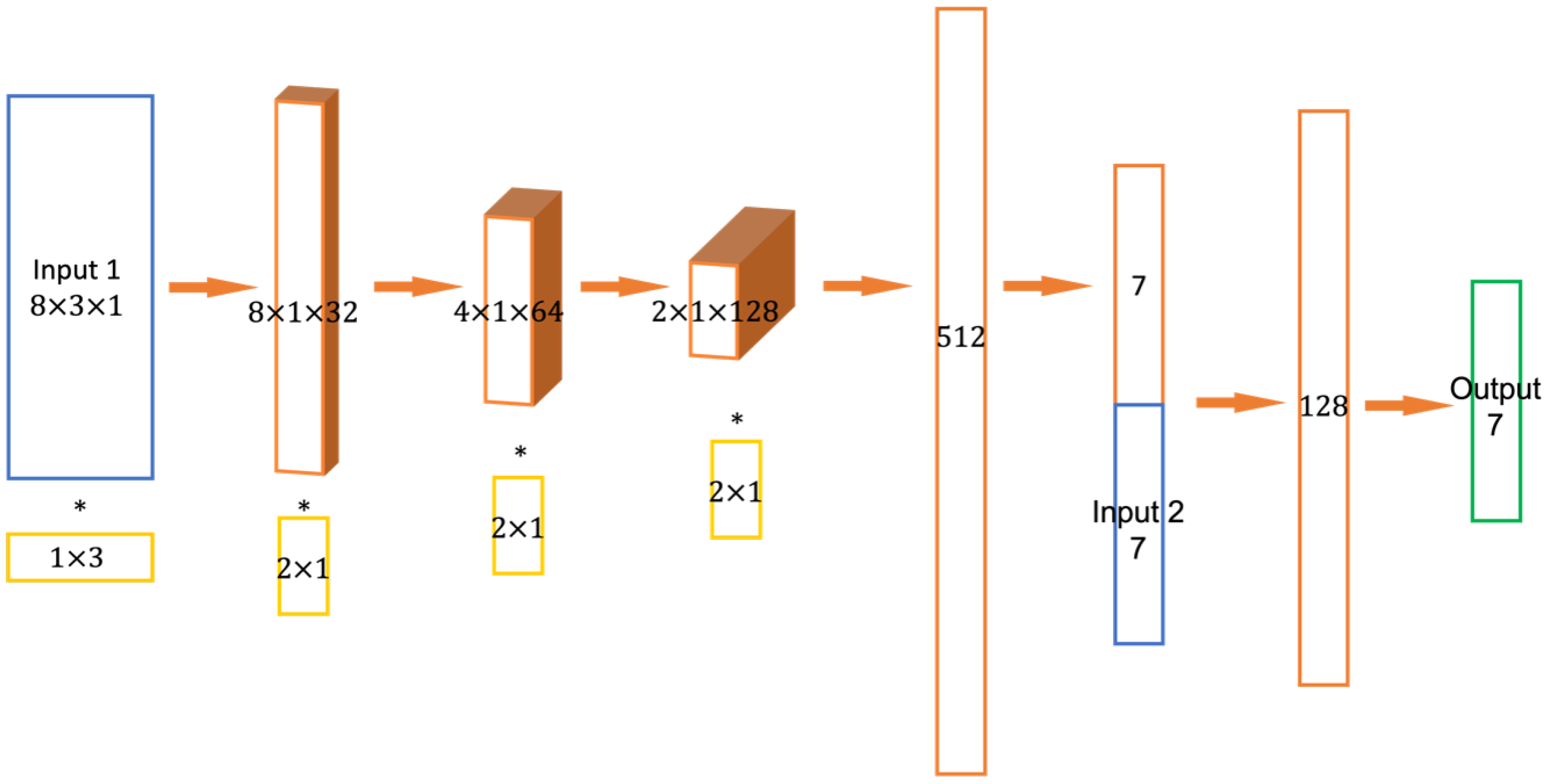
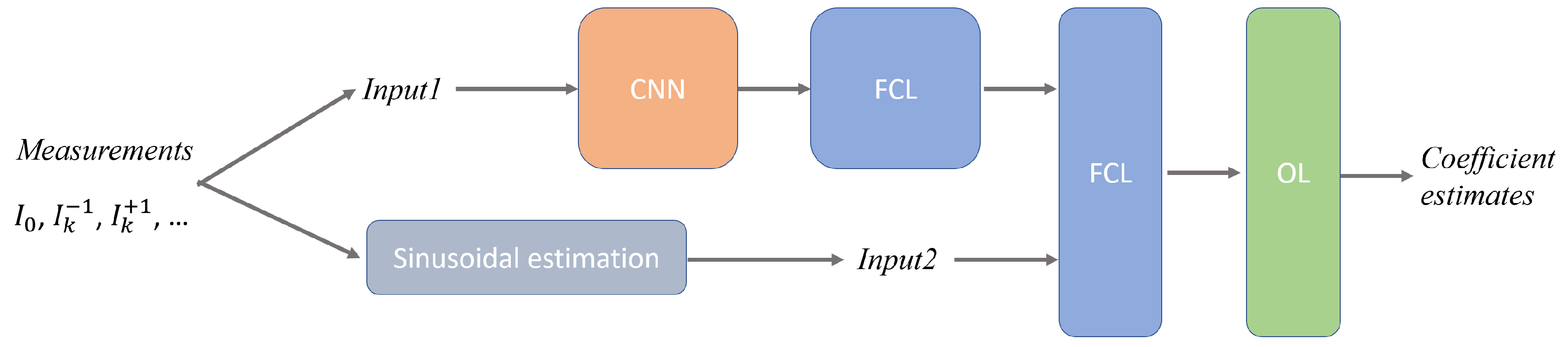
The NN process was constructed as shown in Figure 6; a more detailed description of the architecture is given in Appendix D. The NN takes two separate sets of inputs, both of which rely on biased intensities (generated using Equation (1)): the first (Input1) directly uses these normalised intensity values, while the second (Input2) analytically processes the intensities based upon sinusoidal estimation to acquire a set of preliminary aberration coefficient estimates. The first input is passed into a convolutional neural network (CNN) followed by fully connected layers (FCL). It is then concatenated with the second input (Input2) and passed into fully connected layers to generate the outputs that correspond to the estimated Walsh coefficients. The rationale behind this dual input approach was that the learning task would be easier if based, in effect, on the differences between rough estimates and actual measurements rather than on the raw measurements themselves.
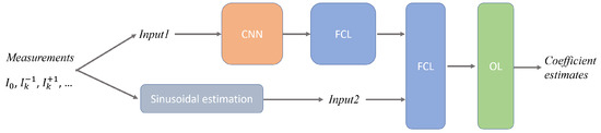
Figure 6.
Outline of the NN architecture and preprocessing of data. CNN: convolutional neural network; FCL: fully connected layer; OL: output layer.
Input1 was structured in the instance of , as a matrix in the following form
This structure was chosen so that the CNN block could interpret known correlations from biased measurement values. Indeed, the first CNN layer was structured so that it operated first on the 3-tuples of intensity values contained in each row of Input1, which were each expected to depend primarily on the corresponding coefficient . Further CNN layers sought to operate on correlations between the different coefficients.
The rough estimation used for Input2 was based upon the knowledge that variations in a single Walsh mode coefficient led to a sinusoidal relationship with detected signal (see Appendix C). The value of each coefficient in Input2 was set to the value that provided the maximum value of this sinusoidal variation. This estimation provides only a rough value for correction, as it treats each coefficient separately and hence does not deal with the coupling effect between combinations of modes.
Separate instances of this NN architecture were trained for the two scenarios. In the first case of the hypercube cell, the training and validation data were obtained by assigning a random value to each input coefficient in the range . For the second case, the same combinations of coefficients were “wrapped” so that they lay only within the primary Voronoi cell (see Appendix D). In each case, the same calculated intensity measurements were used at the input. The difference between the two training processes lies in the coefficient labels that were used to calculate the loss function during network training—in the first case, the coefficient labels were defined throughout the hypercube cell; in the second case, the corresponding labels were wrapped into the primary Voronoi cell. Full details of the training procedure are provided in Appendix D.
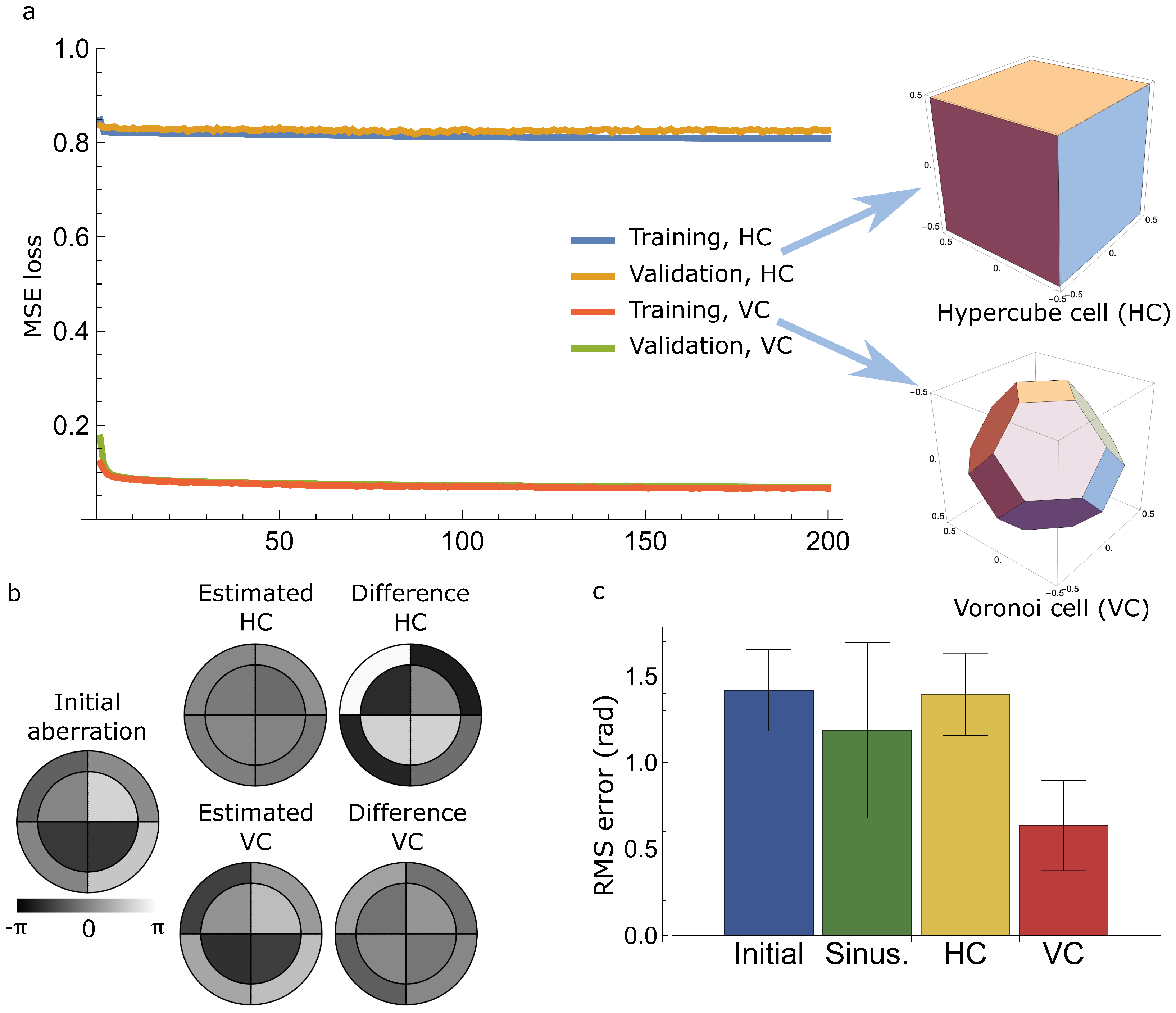
Results are shown in Figure 7 for the case of , which corresponds to the correction of 7 Walsh modes. The loss function curves showed that only the scenario of confining the coefficient to within the primary Voronoi cell permitted the NN to converge. The mean squared phase error was reduced to 0.063 radians after correction, which corresponded to a Strehl ratio of approximately 0.6. In comparison, the loss for the hypercube case was significantly higher and the validation loss did not reduce while deviating from the training loss. This demonstrated the effectiveness of using prior knowledge about the lattice symmetries. It is expected that similar trends would be seen in scenarios with large pixel numbers, alongside more complicated NN architectures.
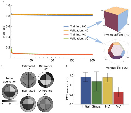
Figure 7.
(a) NN training and validation loss functions as mean square error (MSE) for the scenarios where the coefficient labels were defined throughout the hypercube cell (HC) or the primary Voronoi cell (VC) for . The insets on the right show a schematic representation in three dimensions the difference between the two types of cells. (b) An illustrative example of correction of an initial aberration consisting of 8 pixels, equivalently 7 polar Walsh modes. The residual error of the VC-based correction was far lower than that of the HC based correction. (c) Statistical summary of correction results from the NN validation set: Initial—distribution of initial input aberrations; Sinus—after estimation using sinusoidal model; HC—after correction using the hypercube cell method; VC—after correction with the Voronoi cell method. Error bars show the standard deviation of the distribution.
These results show clearly that the prior knowledge of the lattice geometry, and hence the need to confine the estimation to the primary Voronoi cell, is essential to effective training of the NN. When training using coefficients selected from the hypercube cell, the loss functions (which are related to wavefront estimation errors) do not converge sufficiently to provide good aberration correction. This is attributed to the existence of multiple optimal solutions within the hypercube cell that complicate the training process. However, this problem is avoided when using a training set where the labels were “wrapped” and the resulting labels were within the primary Voronoi cell, and thus only one optimal combination of Walsh mode coefficients is present.
12. Conclusions
The insight provided by the mathematical link between Walsh mode AO and lattices informs the design of efficient sensorless AO schemes. This is relevant to the solution of the inverse problem of how to estimate the aberration coefficients from metric measurements with different applied bias aberrations. The new insights are particularly important when using NNs to solve this inverse problem, as otherwise we suffer from the challenges caused by having multiple solutions for a given set of metric measurements, which requires more complicated networks.
Although the Walsh modes are pixelated, when sufficient pixels are used, they can provide a suitably accurate representation of low order aberrations. While continuous modes, such as the Zernike polynomials, are commonly used, they are not guaranteed to provide a good fit to high-order aberrations in the system, nor to the correction device, which may well be pixelated in nature. The results presented here have relevance not just for correction of low-order aberrations but also for high-order scattering compensation, where previously schemes have been based around control of Walsh modes (or similar) [15,16,17].
The analysis presented in this paper was based around a simple AO focussing system. However, as the overall lattice geometry arises from the nature of the aberration representation, and not the AO system or the optimisation metric, a similar repetitive lattice structure and primary Voronoi cell will hold for any other AO system using Walsh modes as the basis. These results should therefore have relevance to any application of AO using pixelated correction devices.
Author Contributions
Conceptualization: M.J.B.; methodology: M.J.B. and Q.H.; software: M.J.B., Q.H. and Y.X.; validation: Q.H., J.C., R.T. and Y.X.; investigation: M.J.B., Q.H. and Y.X.; writing—original draft preparation: M.J.B. and Q.H.; writing—review and editing: R.T., J.C. and Y.X.; visualization: M.J.B. and Q.H.; supervision: M.J.B.; funding acquisition: M.J.B. All authors have read and agreed to the published version of the manuscript.
Funding
This research was funded by the European Research Council, grant number 695140 (AdOMiS).
Conflicts of Interest
The authors declare no conflict of interest.
Abbreviations
The following abbreviations are used in this manuscript:
| AO | Adaptive optics |
| DM | Deformable mirror |
| SLM | Spatial light modulator |
| NN | Neural networks |
| SNR | Signal to noise ratio |
| AE | Adaptive element |
| CNN | Convolutional neural network |
| FCL | Fully connected layers |
| WT | Walsh transform |
Appendix A. Observations Based upon the Lattice Geometry
Various connections can be made between the operation of the Walsh mode-based AO system and the lattice representation outlined above. The following points address certain relationships between variations of individual pixels and the Walsh functions.
- A single pixel variation is put into effect by a combination of all N Walsh modes, which can be obtained using Equation (5). As is clear from this equation, the coefficients in the vector are themselves given by the elements of a Walsh mode.
- As we have removed the first (piston) mode, we can see that each reduced Walsh mode (i.e., without its first element) is a vector of length that points in the direction corresponding to the variation of a single pixel. As these vectors each include all the basis vectors in equal magnitude (), then these directions must correspond to some of the body diagonals between opposite vertices through the centre of the fundamental cubic cell that encloses the Voronoi cell.
- For N pixels, there are body diagonals that correspond to single pixel variations (counting positive and negative directions separately). For , this is less than the total number of body diagonals, which is . Hence, for , there are diagonals that do not correspond to single pixel variations, but would involve multiple changing pixels.
- The “kissing number” is a characteristic of a lattice that indicates how many nearest neighbours there are to any lattice point. The kissing number for the lattice is (for ), so for we expect (p155 of [10]). This is equal to the number of body diagonals noted above as corresponding to single pixel variations. These single pixel variations correspond to the kissing directions, which are the closest spacing between lattice points.
- Equation (8) shows how I varies with single pixel modulation. However, removal of the piston mode leads to some differences. Ensuring zero piston means that all pixels are modulated, but pixels are shifted by the same value , whereas the single desired pixel will be shifted by the value . The peak-to-peak amplitude would be .
- The mean square amplitude of such a mode must be given byHence, the rms phase related to the peak-to-peak phase by .
- The distance between these closest lattice points is equivalent to the rms phase required to shift one pixel so that it is radians different to the others. Setting gives . This varies inversely with , such that as N increases the spacing between closest lattice points reduces. This is to be expected, as increasing N means a smaller pixel size and hence a smaller rms phase for a given phase variation of a single pixel.
- Along these kissing directions, the minimum signal is obtained when the single pixel is out of phase with the other pixels. This leads to a signal minimum ofwhich tends to 1 as N increases and, correspondingly, as the size of a single pixel decreases.
Hence, we can also use this lattice description to show that the signal varies only weakly in these kissing directions (corresponding to single pixels), whereas adjustment of Walsh modes provides more robust measurement. This confirms the results presented in Figure 3 using single pixel and modal variations. These properties are closely related to the extent of the Voronoi cell in these kissing directions. The Voronoi cell is in effect narrower in the kissing directions than in others. In general, larger signal modulations are obtained if one samples the function in the directions where the Voronoi cell has a larger extent.
Appendix B. Sensorless AO and the Walsh Transform
Suppose we take a sequence of biased measurements, where we apply biases of each Walsh mode with a single positive amplitude of radians. This is equivalent to shifting the measurement point from the body centre of the ()-dimensional Voronoi cell to the centre of each ()-dimensional facet centred along the positive axis of the corresponding Walsh mode. Due to the lattice structure, the facet in the positive direction is homologous to the facet in the negative direction. Therefore, by choosing this bias amplitude, we are simultaneously sampling both the positive and negative bias positions. When biasing the kth mode, we are increasing the (unknown) coefficient by . The complex pixel value of that mode is therefore
where we have exploited the fact that the Walsh function has values only of . We can now see that the kth biased signal measurement is given from Equation (7) by
where we have defined to represent the complex pixel values so that:
The Walsh transform (WT) of a sequence of length N is defined conventionally as [8]:
We can therefore derive
In other words, we see that the set of biased intensity measurements is the modulus squared of the kth component of the WT of the complex pixel values . As the first Walsh function is piston (hence all pixels have value 1), it is related to the first element of the WT . As biasing with piston has no effect on the measurement, this is the same as the unbiased measurement in our system. Hence, the unbiased measurement (corresponding to the centre of the Voronoi cell) along with the biased measurements correspond to a full set of intensity measurements. This set of intensity measurements is known as the spectral density of the WT of the set of complex pixel values. In practice, we cannot measure the complex values of directly, but we are able to quantify the Walsh spectral density through the intensity measurements with the applied bias modes.
We now derive a relationship using the fundamental properties of the WT. In [8], we find an equivalent of Parseval’s theorem for WTs:
From the definition of , it is clear that its modulus is equal to one. Hence, we find that
Equivalently, we find that the sum of the biased measurements and the one unbiased measurement must add to one.
The importance of this result is that in a real experiment the measured signal is not actually normalised to one, but there is an unknown “brightness” that is a function of numerous experimental variables. This would be a multiplying factor in the expressions for I, which we have chosen to omit from the analysis for simplicity. We can use this result to obtain the “brightness” in a way that is independent of the input aberration, as it is simply the sum of the biased measurements and the unbiased measurement.
Appendix C. Estimation of Coefficients Using Simple Sinusoidal Model
In this appendix, we present a method for rough initial estimation of individual Walsh mode coefficients. Let us redefine Equation (7) by including a factor A that is equivalent to an unknown maximum intensity
The signal varies with a single modal coefficient as
where the effects of the modes contained within the first exponential term have been subsumed into the complex coefficients .
We introduce a useful relationship, which takes advantage of the binary () values of the Walsh functions [9]:
This leads to
The exact form of this solution will depend upon and hence on the other Walsh coefficients. However, the only terms in that can arise from the modulus square term are of the form of , , or , which can all be expressed as sinusoidal terms of argument . Hence, we deduce that must be given by the form
where p, q and depend on all values . Let us simplify Equation (A14) to the form , where we have defined .
Consider applying a bias so that the biased measurement . Then, we apply the negative bias so that the biased measurement . We also use the unbiased measurement . If we use a bias of , then we can obtain through elementary operations
The value of obtained through Equation (A15) was used as the initial rough estimate provided to the NN as Input2. The error between this estimate and the actual coefficient is given by .
Appendix D. Description of the Neural Network Training and Network Architecture
The training data consisted of (about one million) simulated samples, and (128) samples were used for validation to avoid overfitting. Both sets of data were generated for the case of , corresponding to the correction of seven Walsh modes (excluding piston). The total number of training datasets was chosen to provide a sufficient representation of the seven-dimensional search space.
For each training dataset, seven values were randomly generated corresponding to the coefficients of seven polar Walsh modes (). The coefficients followed a uniform distribution over the range of to . These coefficients were used as labels during network training in the case of the hypercube cell.
The sum of the product between each coefficient with its corresponding unit Walsh mode formed the phase aberration according to Equation (3). The phasor of the complex field was calculated by averaging the complex field over the pupil. By subtracting the angle of the mean phasor of across the pupil (Equation (A16) ) and wrapping the phase back within the range of , the aberration was calculated to be equivalent to and within the primary Voronoi cell.
Using the orthogonality of Walsh modes, the new coefficients of the equivalent aberration (Equation (A17)) could be calculated. were used as the labels when training the network with a confined searching space.
For each set of data, two phase biases per Walsh mode were introduced. The bias amplitudes were chosen to be and . For each introduced bias phase, the intensity signal ( and ) was computed using the Equation (1). The same equation was used to calculate the signal when no bias phase was introduced (). From previous discussions, the phase modulation of mode 1 (piston) would have no effect on the signal and thus excluded from the collection of signal readings. The total of 15 signal readings (14 biased and 1 unbiased readings) were used as the input (Input1) of the network.
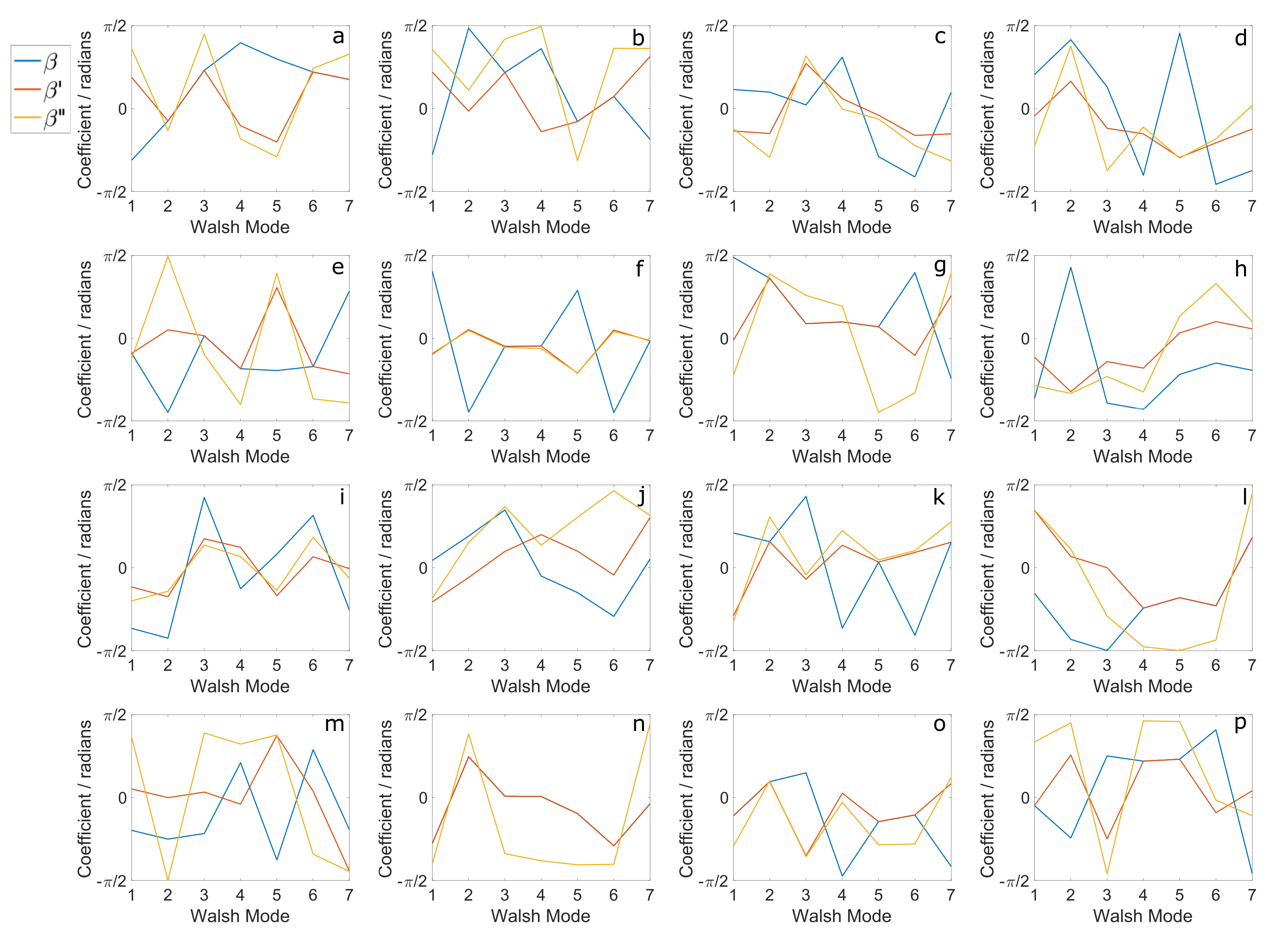
In addition, from our previous discussion, the signal varied with mode coefficients in a period of . A good approximation to the coefficients of each mode () was obtained using Equation (A17). These approximations were also used as the separate input (Input2) to the two networks we trained. Figure A1 shows a few sets of , and , which derived from the same initial aberration.
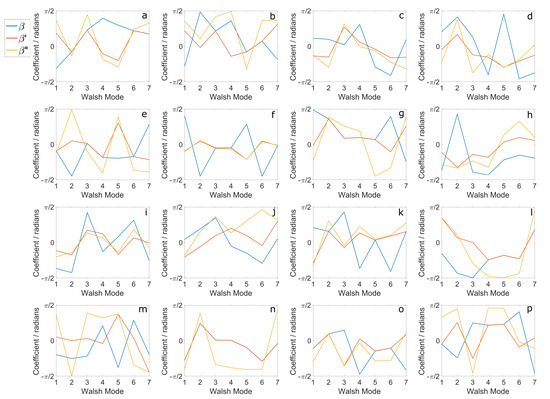
Figure A1.
(a–p) 16 sets of randomly selected , and derived from the same aberration, shown in blue, red and yellow plots, respectively. In some cases, (estimation using sinusoidal model) closely resembled (such as in case (f)) while in some other cases, could be different to (such as in (e) and (n)). There were also a small proportion of cases where was identical to (such as (n)), which corresponded to the initial aberration being within the primary Voronoi cell.
The full diagram of the NN architecture is shown in Figure A2. The network was built using TensorFlow Keras. For the first CNN layer, the padding was chosen to be “valid” and strides equalled to (1,1). For each of the second to fourth CNN layers, the padding was chosen to be “same” and strides equalled to (1,1). Following each of the second to the fourth convolutional layers was a maxpooling layer with a pool size of . For all the layers (except the output layer), the nonlinear activation was chosen to be “tanh”. The activation of the last output layer was linear. The initializer of all the kernels was glorot uniform. The loss function was mean squared error (MSE). The optimizer was Adam.
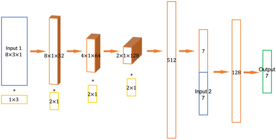
Figure A2.
Full neural network architecture. The blue boxes were the two inputs to the network. The yellow boxes were the trainable kernels of the CNN with the corresponding dimensions as shown. The orange boxes were the internal layers of the CNN and dense layers in the later stages. The green box represents the output of the CNN.
References
- Booth, M.J. Adaptive optical microscopy: The ongoing quest for a perfect image. Light Sci. Appl. 2014, 3, e165. [Google Scholar] [CrossRef]
- Ji, N. Adaptive optical fluorescence microscopy. Nat. Methods 2017, 14, 374–380. [Google Scholar] [CrossRef] [PubMed]
- Hampson, K.M.; Turcotte, R.; Miller, D.T.; Kurokawa, K.; Males, J.R.; Ji, N.; Booth, M.J. Adaptive optics for high-resolution imaging. Nat. Rev. Methods Prim. 2021, 1, 68. [Google Scholar] [CrossRef] [PubMed]
- Booth, M.J.; Neil, M.A.A.; Juškaitis, R.; Wilson, T. Adaptive aberration correction in a confocal microscope. Proc. Natl. Acad. Sci. USA 2002, 99, 5788–5792. [Google Scholar] [CrossRef] [PubMed] [Green Version]
- Hu, Q.; Wang, J.; Antonello, J.; Hailstone, M.; Wincott, M.; Turcotte, R.; Gala, D.; Booth, M.J. A universal framework for microscope sensorless adaptive optics: Generalized aberration representations. APL Photonics 2020, 5, 100801. [Google Scholar] [CrossRef]
- Facomprez, A.; Beaurepaire, E.; Débarre, D. Accuracy of correction in modal sensorless adaptive optics. Opt. Express 2012, 20, 2598–2612. [Google Scholar] [CrossRef] [PubMed] [Green Version]
- Saha, D.; Schmidt, U.; Zhang, Q.; Barbotin, A.; Hu, Q.; Ji, N.; Booth, M.J.; Weigert, M.; Myers, E.W. Practical sensorless aberration estimation for 3D microscopy with deep learning. Opt. Express 2020, 28, 29044–29053. [Google Scholar] [CrossRef] [PubMed]
- Beauchamp, K. Walsh Functions and Their Applications; Nutrition, Basic and Applied Science; Academic Press: Cambridge, MA, USA, 1975. [Google Scholar]
- Wang, F. Wavefront sensing through measurements of binary aberration modes. Appl. Opt. 2009, 48, 2865–2870. [Google Scholar] [CrossRef] [PubMed]
- Conway, J.H.; Sloane, N.J.A. Sphere Packings, Lattices and Groups, 3rd ed.; Grundlehren der mathematischen Wissenschaften, A Series of Comprehensive Studies in Mathematics; Springer: New York, NY, USA, 1999; Volume 290. [Google Scholar]
- Booth, M.J. Wave front sensor-less adaptive optics: A model-based approach using sphere packings. Opt. Express 2006, 14, 1339–1352. [Google Scholar] [CrossRef] [PubMed] [Green Version]
- Antonello, J.; Verhaegen, M.; Fraanje, R.; van Werkhoven, T.; Gerritsen, H.C.; Keller, C.U. Semidefinite programming for model-based sensorless adaptive optics. J. Opt. Soc. Am. A 2012, 29, 2428–2438. [Google Scholar] [CrossRef] [PubMed] [Green Version]
- Weisstein, E.W. Hadamard Matrix—From Wolfram MathWorld. Available online: https://mathworld.wolfram.com/HadamardMatrix.html (accessed on 18 July 2022).
- Sloane, N.J.A. Hadamard Matrices. Available online: http://neilsloane.com/hadamard/ (accessed on 18 July 2022).
- Tang, J.; Germain, R.N.; Cui, M. Superpenetration optical microscopy by iterative multiphoton adaptive compensation technique. Proc. Natl. Acad. Sci. USA 2012, 109, 8434–8439. [Google Scholar] [CrossRef] [PubMed] [Green Version]
- Park, J.H.; Sun, W.; Cui, M. High-resolution in vivo imaging of mouse brain through the intact skull. Proc. Natl. Acad. Sci. USA 2015, 112, 9236–9241. [Google Scholar] [CrossRef] [PubMed] [Green Version]
- Kong, L.; Cui, M. In vivo neuroimaging through the highly scattering tissue via iterative multi-photon adaptive compensation technique. Opt. Express 2015, 23, 6145–6150. [Google Scholar] [CrossRef] [PubMed]

Publisher’s Note: MDPI stays neutral with regard to jurisdictional claims in published maps and institutional affiliations. |
© 2022 by the authors. Licensee MDPI, Basel, Switzerland. This article is an open access article distributed under the terms and conditions of the Creative Commons Attribution (CC BY) license (https://creativecommons.org/licenses/by/4.0/).