Abstract
Satellite vibration is an important factor that can seriously reduce the image quality of remote sensing imaging. In this paper, the influence of the random vibration of the payload on the frame-by-frame imaging quality of the area-array CMOS camera is studied. Firstly, the mode of the camera’s dynamic frame-by-frame imaging is established; secondly, the curvature mapping function between the ground and camera focal planes is derived based on the invariance of the field of view (FOV). The frequency domain-filtered template of random vibration is constructed. Then, the distortion and degradation images, of single-frame images at different attitude angles, are inversed; finally, the influence of attitude angle, exposure time, and the error of velocity, caused by random vibrations on dynamic frame-by-frame imaging, are analyzed. The simulation results show that the degree of image edge distortion gets larger when the attitude angle increases from 0° to 50°. At the same time, the MTF decreases rapidly with the increase of the error of velocity and the attitude angle. Meanwhile, when the output-image SSIM decreases by 0.1, the MSE increases by 18.5. The experimental results show that the field of view (FOV) of dynamic imaging should be reasonably set, and the error of velocity should be effectively reduced to obtain high-quality remote sensing images.
1. Introduction
Space-based remote sensing technology has important significance and application in national construction and urban planning [1,2,3]. Coverage has always been an important indicator for evaluating high-resolution aerospace images. Technologies, such as multi-satellite networking, multi-camera stitching [4], and agile satellite imaging, have effectively increased the coverage of remote sensing images [5]. However, the burden of the space payload has also increased. In order to reduce the weight of payload, a dynamic frame-by-frame imaging mode, in which an optical camera and an oscillating mirror cooperate with each other, has been proposed by scholars [6,7]. In this mode, the mutual restriction between the aperture and focal length of the optical system, which can realize high-resolution and large-width imaging, has been broken. However, the multi-mechanism cooperative motion will have more random interference factors, which can affect the stability of the dynamic velocity and reduce the quality of the image in this dynamic imaging mode [8]. Therefore, it is necessary to further systematically analyze the law of image degradation in the dynamic imaging process.
In the process of remote sensing imaging, mechanical vibrations lead to the lower precision of the accurate alignment system and the instability of the tracking system, which seriously affect the quality of satellite imaging [9]. So far, researchers have analyzed the effect of satellite vibration on imaging quality in traditional imaging mode. The optical system function (OTF) of linear vibration and sine vibration on the image plane were derived by Hadar et al. [10,11]. Adrian et al. [12] further proposed a method for calculating OTF with no limitation of any specific satellite vibration type, and the formula of the modulation transfer function (MTF) was extended to the full frequency range by Du et al. [13]. Since the total MTF was reduced by spatial vibration, a frequency domain filtering system, which included various vibration types, had been mentioned by Deng [14] and Li et al. [15] to simulate the image degradation phenomenon caused by the multi-source vibration of the payload.
In recent years, many new modes of dynamic imaging have been proposed in order to improve the imaging width and resolution. A circular-scanning imaging model was established by Song et al. [16]. By setting a reasonable scanning speed, the overlapping output of multi-frame images was completed to maximize the imaging coverage of the camera. Zhong et al. [17] further described the optical rotation phenomenon between the object and the image, in the circular scanning imaging model, by establishing different coordinate systems, so the imaging model of the circular scanning sensor tended to be mature. Liu [18] et al. proposed a scanning mirror system, which consisted of an objective lens, relay lens, and three-stage imaging lens, to simulate the relationship between objects and images in a two-dimensional scanning motion. It provided a theoretical basis for the structural design of the scanning mirror. Meanwhile, Tianqing et al. [19] established an experimental dynamic scanning imaging system with fast steering mirrors, which was used to monitor hot targets and scout hot areas in real time. With the increase of the scanning attitude angle, the output image was seriously distorted. Ng et al. [20] confirmed that imaging distortion could be corrected by measuring the four polarization directions of polarization imaging. In the scanning imaging system, using a camera’s front mirror, Lu [21] further expounded on the design scheme from two aspects: structure and the control circuit. In this system, the encoder read the payload attitude information when the mirror of the camera periodically scanned.
With the development of dynamic optical imaging technology, the vibration analysis of traditional imaging can’t meet the actual requirements. Therefore, it is necessary to further study the law of image degradation, caused by vibration, in the new dynamic imaging mode. During the frame-by-frame imaging process, the internal disturbance source of the payload randomly vibrates irregularly. When random vibration is coupled with the disturbance characteristics of the dynamic frame-by-frame imaging model, new problems will appear. In order to solve the above problems, a periodic dynamic frame-by-frame imaging model of the CMOS camera is established in this paper. The pixels’ curvature mapping function, between the payload CMOS camera and the ground imaging range, is derived according to the invariance of the field of view. The error of velocity, caused by random vibration, is introduced into the camera focal plane to invert the image degradation phenomenon in the process of dynamic imaging and to quantitatively analyze the quality of space remote-sensing images in a complex space environment.
2. Model of Dynamic Imaging
2.1. Dynamic Frame-by-Frame Imaging Models
In order to expand the ground imaging range, the SiC mirror rotates periodically in front of the CMOS camera scans, at a certain velocity, in the dynamic imaging mode [22]. In this process, the dynamic frame-by-frame imaging schematic is established, as shown in Figure 1.
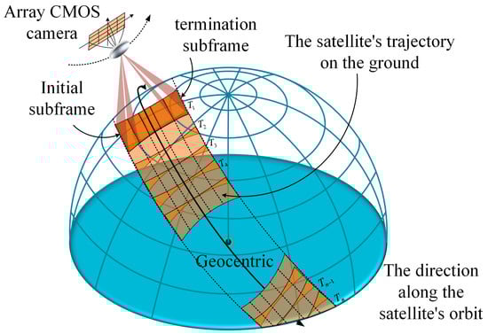
Figure 1.
Schematic diagram of dynamic frame-by-frame imaging.
When the satellite flies to the observation area along the orbit, the mirror rotates with a certain angular speed at the initial position, and the initial sub-frame image is exposed at T1. The exposure time interval is calculated by satellite, according to the single frame width, and then, the single-frame images along the vertical track direction are obtained according to the time interval T2, T3…Tn. Finally, the extended-amplitude image can be gained after splicing all the frame images according to the time sequence. However, the ground area, covered by CMOS pixels, changes from a square to an approximate trapezoidal image, with different sizes, as the imaging attitude angle increases in the dynamic imaging mode. At the same time, the anisotropic motion between pixels leads to serious distortion of the image on the CMOS focal plane. In addition, the internal rigid structure, when subjected to dynamic disturbance, produces serious random vibration. It makes the CMOS focal plane deviate from the target image by a certain angle, resulting in the degradation of image quality. For the sake of effectively analyzing the distorted output image and the degraded image caused by random vibration in the dynamic frame-by-frame imaging process, the imaging simulation link is established, as shown in Figure 2.
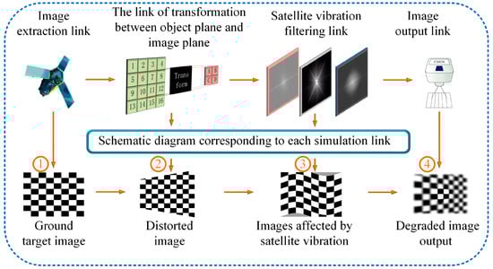
Figure 2.
Simulation link for dynamic imaging.
The ground target image is obtained by one exposure of the camera, as shown in Figure 2①, where the pixel’s coordinate function is . According to the invariance of the field of view, distortion image on the camera’s focal plane is obtained, as shown in Figure 2②, where the pixel’s coordinate function is . The generalized function is expressed as the transformation operation between the ground target and the distorted image on the camera focal plane, so the mapping relationship can be expressed as:
The degraded image can be obtained by the convolution of the distorted image function and the line spread function , which is caused by satellite vibration, as shown in Figure 2③.
In the formula, is the degraded image interfered by random vibration. With the transformation of the Fourier transform, the frequency domain calculation formula is expressed as:
where, is the output-image spectrum; is the input image spectrum; is called the modulation transfer function, which is the Fourier transform of the line spread function caused by random vibration.
It represents that the different frequency components are modulated by the filtering system. The distortion degraded image is obtained by the inverse Fourier transform of the output-image spectrum , as shown in Figure 2④.
2.2. The Exposure Equation of CMOS Camera
The synchronization between the ground imaging efficiency and the reading efficiency of the pixels on the camera focal plane is the premise of high-resolution imaging [23]. According to the object–image mapping relationship, the exposure time of the CMOS camera in the dynamic frame-by-frame imaging process is defined as the function of the ground resolution and the ground imaging velocity , which can be expressed as follows:
As shown in Figure 3, an instantaneous imaging model is established by taking the single-frame image at the moment T1 in Figure 1 as an example. The expression of the geocentric angle and the camera object distance can be calculated from the trigonometric function:
where, is the radius of the earth and is the height of the satellite orbit. According to the relationship among camera object distance , focal length , and pixel size , the ground resolution calculation formula can be expressed as:
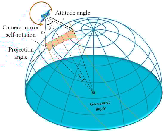
Figure 3.
Schematic diagram of overall dynamic frame by frame imaging.
Since the imaging velocity of the camera on the ground is combined velocity , which consists of camera scanning velocity and satellite flight velocity , it can be expressed as:
In the formula, is the gravitational constant and M is the mass of the earth. It can be supposed that the number of the imaging line of the area-array CMOS camera is N, while the exposure time of the area-array camera, at different attitude angles, can be expressed as:
2.3. Curvature Distortion Mapping Function of Ground Pixels
For explaining the curvature mapping relationship between the ground target image and camera focal plane image, the local frame-by-frame imaging model between the object and the image is established, as shown in Figure 4.
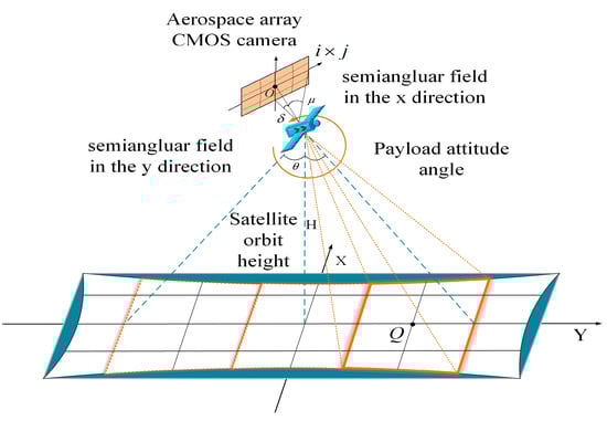
Figure 4.
Schematic diagram of local dynamic frame-by-frame imaging.
Firstly, the phase coordinate system is set, in which the center of the focal plane of the CMOS camera is the coordinate origin . There are imaging units on the phase surface (the number of imaging units in the X direction is i, and the number of imaging units in the Y direction is ). Secondly, the object plane coordinate system is set, in which the center point of the ground imaging area is the coordinate origin . Then, the field angle and of any pixel point in the X direction and the Y direction on the camera focal plane can be expressed as:
In the formula, is the focal length of the camera, is the pixel size, while and are the X and Y components of the target pixel in the phase coordinate system, respectively. Then, any pixel point in the object plane coordinate system can be expressed as:
In the formula, and are X and Y components of target pixel point in the object plane, respectively. Combining Formulas (13) and (14), the curvature mapping function , which represents the relationship between the ground target image and the phase surface distortion image, can be expressed as:
2.4. Frequency Domain Image Filtering of Random Vibration
In the process of frame-by-frame imaging, a certain error of velocity of the optical camera is caused by the multi-source vibration of the aerospace payload, which is transmitted to the camera focal plane through the mechanical structure. After camera exposure, such error image shifts can sharply destroy the output image sharpness. If the input image is a gaussian image, the line spread function , caused by random vibration, can be expressed as:
The MTF of the filter system is obtained by the Fourier transform of the :
In a linear system, the function of the MTF is approximated to be a digital filter, which is called a filter template. It realizes the response to various frequency components of the input spectrum in an image filtering system, and the output image spectrum can be obtained from Formula (3)
The degraded image can be obtained by the inverse Fourier transform of the output image spectrum:
where and indicate that the size of the input image is .
2.5. Image Sharpness Evaluation
SSIM and MSE are common image sharpness assessment tools that can compare the difference between two images of the same size. After the degraded image of the frequency domain filtering is obtained, SSIM and MSE are used to analyze the regularity of image quality degradation caused by satellite vibration.
The formula for SSIM is expressed as:
where is brightness distortion; is contrast distortion; is structural distortion. , , and are the corresponding weight coefficients, respectively. The value range of SSIM is [0, 1]. The larger the value of SSIM is, the smaller the image distortion is.
The formula for MSE is expressed as:
where and are the pixel values of the reference image, and the evaluated image at M and N are also the image size. The higher the value of MSE is, the greater the degree of the distortion is.
3. Results
Based on the above theoretical model, the degradation phenomenon of the output image is simulated and analyzed in the dynamic frame-by-frame imaging process. The parameters of the dynamic imaging model are set, as shown in Table 1:

Table 1.
Simulation parameters.
3.1. Ground Vibration Test
In the dynamic frame-by-frame imaging process, the certain error of velocity, caused by random vibration, has occurred in the mechanical structure. The error of velocity leads to the imaging shift on the camera focal plane within the exposure time, which directly causes the image blur. Therefore, it is necessary to analyze the influence of the error of velocity caused by satellite vibration on dynamic imaging.
In the ground test platform, the multi-cycle tracking velocity is obtained, as shown in Figure 5a, where the blue curve is the actual tracking velocity, and the red curve is the ideal tracking velocity. It can be seen that there is a certain error between the actual velocity and the ideal velocity from Figure 5a. Based on the error analysis of the ground tracking velocity, the curve of the error of velocity is obtained, as shown in Figure 5b, where the error of velocity peaks at different frequencies have been marked.
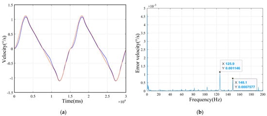
Figure 5.
Ground platform test data. (a) Ground tracking velocity test curves, (b) The error of velocity image.
Five pieces of data are extracted in the actual error of the velocity range (0.0007577°/s, 0.001146°/s); meanwhile, the influences of different error velocities and attitude angles on the MTF of the system are analyzed in the following part.
3.2. Analysis of Ground Distortion Imaging
During the imaging process of the dynamic scanning mirror, the payload’s attitude angle changes periodically. When the angle between the optical axis of the camera and the satellite nadir gets larger, the ground imaging range, corresponding to CMOS pixels, gradually increases. It leads to the anisotropy of motion between pixels and the distortion of images projected onto the focal plane of the camera. In order to simulate this image, a unit pixel is set in every 30 pixels, which represents the pixel-number of the ground image. The arrows represent the direction of movement of the ground image during the imaging process. The distortion diagram of the ground pixels, at attitude angles of 0°, 30°/−30°, and 50°/−50°, can be calculated by the curvature mapping function (15), as shown in the Figure 6.
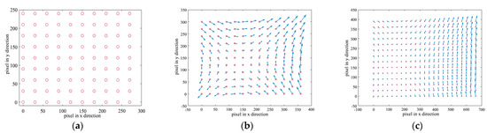
Figure 6.
Schematic diagram of distorted image. (a) Attitude angle 0°, (b) Attitude angle 30°/−30°, (c) Attitude angle 50°/−50°.
It can be seen that, when the attitude angle of satellite is 0 °, the ground imaging range is about 300 pixels × 250 pixels. It indicates that the ground imaging range is narrow, and there is almost no image distortion, as shown in Figure 6a. When the satellite attitude angle gradually increases to 30 ° or 50 °, the ground imaging range becomes 400 pixels × 350 pixels or 700 pixels × 450 pixels. It can be seen that, when the attitude angle increases, the ground imaging range becomes wider, and the image distortion deepens, as shown in Figure 6b,c.
3.3. Analysis the MTF of Sub-Satellite Point Imaging Interfered by Random Vibration
When the attitude angle of satellite is 0°, both the ground resolution GSD and the ground scanning velocity Vc are fixed values. Based on Formula (10), the exposure time is t = 0.0051 s. The MTF curves of different error velocities are simulated, as shown in Figure 7.
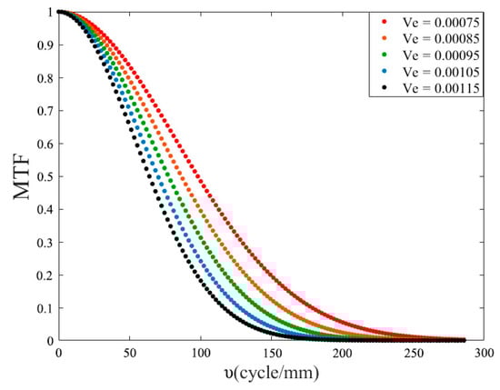
Figure 7.
MTF curves at different error velocities.
It can be seen that, when the velocity error is caused by random vibration increases, the error image shift on the focal plane of the camera gets larger. Therefore, the MTF curve shows a significant downward trend, which means that the clarity of the output image is reduced.
3.4. Analysis the MTF of Dynamic Imaging Interfered by Random Vibration
In the dynamic frame by frame imaging system, the attitude angle of the camera will change periodically. In this process, the exposure time of the camera is different when the attitude angle of satellite varies at different velocities. Therefore, it is necessary to calculate the exposure time of subframes with different attitude angles. According to Equation (10) and the parameters in Table 1, the exposure time of the camera at different angles is simulated, as shown in Figure 8.
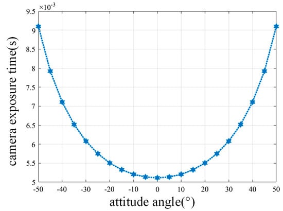
Figure 8.
Camera exposure function.
It can be seen that the camera exposure time becomes larger as the satellite attitude angle increases during the single-frame imaging in Figure 8.
In order to analyze the influence of the error of velocity and attitude angle θ on MTF, spatial frequency is set as the Nyquist frequency , and then, the MTF is transformed into:
The MTF curves with different error velocities and attitude angles are obtained, as shown in Figure 9.
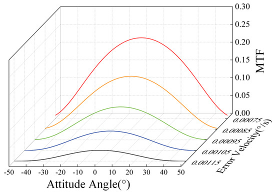
Figure 9.
MTF curves of dynamic frame-by-frame imaging.
Comparing Figure 7 and Figure 9, it can be seen that there are similar conclusions in the dynamic imaging model and the satellite nadir imaging model: When the camera’s attitude angle is set as a fixed value, the MTF decreases with the increasing error of velocity.
However, when the error of velocity is set as a fixed value, the MTF value achieves its maximum at the attitude angle 0°. When the optical axis of the camera deviates from the satellite nadir, MTF decreases significantly, so it appears to be an approximate “arch” in the MTF curves.
It can be explained that the exposure time of the camera at the satellite nadir is the shortest. With the increasing attitude angle, the exposure time of the camera becomes longer. When the camera is disturbed by the error of velocity, caused by random vibration, the error image shift on the camera focal plane is limited by the short exposure time. With the increasing attitude angle, the error image shift in the camera focal plane becomes larger due to the long exposure time. The more error image shifts are introduced into the focal plane of the camera, the more significantly the MTF drops. Therefore, the image quality of the sub-frames, farther from the satellite nadir, is degraded more obviously in a group of single-frame wide-frame images.
3.5. Remote Sensing Image Simulation
In this section, the mechanism of image distortion of the curvature map and image degradation, caused by satellite random vibration, have been explained. Firstly, the high-resolution ground image is converted by the ground curvature mapping Formula (15), and the distorted image on the camera focal plane is obtained; secondly, the distorted image is filtered in the frequency domain by the filter template (18) and, then, by the Fourier inverse transform (19). Finally, the degraded image is obtained.
In the coaxial plane optical system, the image degradation result, in the direction along the track and the vertical track, is the same. Then, the system filter template (18) can be expressed as:
where the error of velocity, caused by random vibration, is set to 0.00076°/s. Then, the frequency domain-filtered template images, at attitude angles of 0°, 30°/−30°, and 50°/−50°, are simulated, as shown in Figure 10. It can be seen that the image filtering has the same effect when the attitude angle is symmetrical about the position of the satellite nadir.
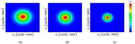
Figure 10.
Image filter template: (a) attitude angle 0°; (b) attitude angle 30°/−30°; and (c) attitude angle 50°/−50°.
In order to intuitively describe the actual image degradation phenomenon, the high-resolution ground target image, with a size of 2200 pixel × 400 pixel, is used as the original image. The sub-frame images at attitude angles of −50°, −30°, 0°, 30°, and 50° are assumed to be the stitching units for wide-format imaging. After being filtered by the template shown in Figure 10, the images interfered by random vibration at different attitude angles can be obtained, as shown in Figure 11. The first line is the original image, the second line is the distorted output image on the camera focal plane, and the third line is the degraded image caused by the satellite vibration.
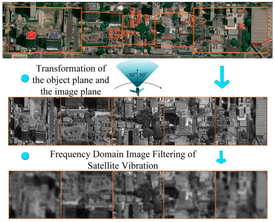
Figure 11.
The simulation process of remote sensing image degradation.
From the first line of Figure 11, it can be seen that the imaging range of the satellite nadir is the smallest. As the angle between the optical axis of the payload and the position of the satellite nadir increases, the imaging range of the area–array camera on the ground becomes wider. From the second line of Figure 11, it can be seen that the degree of image distortion far from the satellite nadir is greater, while the size and scale of the target image get bigger, and the disturbance factor has more influence on the image clarity. From the third line of Figure 11, it can be seen that satellite vibration seriously affects the quality of remote sensing images. Image sharpness evaluation indicators, SSIM (structural similarity) and MSE (mean square error), are usually used to evaluate the degree of image degradation. The higher the value of MSE is, the greater the degree of distortion is. The value range of SSIM is [0, 1]. The larger the value of SSIM is, the smaller the image distortion is. The data of SSIM and MSE, at different attitude angles, are listed in Table 2. When the attitude angle is 0°, the SSIM value is 0.3136, and the MSE value is 76.7977. With the attitude angle increasing to 30° and 50°, SSIM decreases, and the MSE increases, which indicates that, when the error of velocity is the same, the image sharpness decreases with the increasing of the deviation angle between the payload optical axis and the satellite nadir position.
Table 2.
The results of image sharpness evaluation.
4. Discussion
Different from traditional push-broom imaging modes, the degraded image of dynamic scanning mirror imaging, caused by satellite vibration, is analyzed in this paper. In this dynamic imaging model, the image quality will be influenced by the linkage between the satellite and the payload. Therefore, the vibration mechanism of the frame-by-frame imaging model is more complex. In order to simplify the complex relationship of the model, the disturbance of the satellite is displayed by the random vibration factors, and the disturbance of the payload is displayed by the periodically changing attitude angle factors. Then, the frequency domain-filtered template of random vibration is constructed. The following results can be obtained by simulating the dynamic imaging process with the orbital height 500km and the scanning velocity 10°/s of the mirrors in front of the space camera:
- In the process of dynamic imaging, the ground image information becomes larger, and the distortion degree of the output image on the focal plane grows larger with the increasing angle between the optical axis of the camera and the position of the satellite nadir.
- When the attitude angle is a certain value, the MTF drops rapidly with the increasing error of velocity.
- The camera exposure time is determined by the periodically changing attitude angle. When the scanning mirrors scan at the satellite nadir, the camera exposure time is the shortest. With the increasing angle between the optical axis and the satellite nadir, the camera exposure time is extended. When the error of velocity is a certain value, the MTF drops with the axis of symmetry of the satellite nadir.
- In a group of wide, single-frame output images, the error of velocity is caused by the random vibration of the payload mechanism, resulting in an error image shift on the focal plane of the camera. In a set of single-frame images that constitute wide-format imaging, the distortion effect and degradation degree of each single-frame image are different. The single-frame image far away from the satellite nadir has the largest distortion, and the image degradation phenomenon is obvious.
5. Conclusions
To summarize, the wide image output by the CMOS camera with a scanning mirror is simulated in this paper. The degradation law of high-resolution large-width imaging, interfered with by satellite random vibrations, is analyzed. The simulation result shows that the camera exposure time is extended when the payload attitude angle is increasing during dynamic imaging. Further, the degree of image distortion on the camera focal plane becomes larger at locations far away from the satellite nadir. The error of velocity, caused by random vibration, increases the shift amount of an image on the camera focal plane, which directly reduces the image quality. Therefore, the field of view (FOV) should be reasonably set, and the damping mechanism should be installed to obtain a high resolution large-width image.
Author Contributions
Conceptualization, L.J.; methodology, L.J.; software, L.J.; validation, Z.Y. (Ziqi Yu); formal analysis: L.J. and Z.Y. (Zhihai Yao); investigation, Z.Y. (Zhihai Yao); resources, L.J.; data curation, Z.Y. (Ziqi Yu); writing—original draft preparation, Z.Y. (Ziqi Yu); writing—review and editing, L.J., Z.Y. (Ziqi Yu) and K.L.; visualization, Z.Y. (Ziqi Yu). All authors have read and agreed to the published version of the manuscript.
Funding
This research was funded by the National Natural Science Foundation of China (NSFC), grant number 62101071 and 62171430. This research was funded by the Natural Science Foundation of Jilin Province, grant number 20210101099JC and 20210101186JC.
Institutional Review Board Statement
Not applicable.
Informed Consent Statement
Not applicable.
Data Availability Statement
Not applicable.
Acknowledgments
The authors would like to thank National Natural Science Foundation of China.
Conflicts of Interest
The authors declare no conflict of interest.
References
- Zhu, Z.; Zhou, Y.; Seto, K.C.; Stokes, E.C.; Deng, C.; Pickett, S.T.A.; Taubenböck, H. Understanding an urbanizing planet: Strategic directions for remote sensing. Remote Sens. Environ. 2019, 228, 164–182. [Google Scholar] [CrossRef]
- Tomás, R.; Li, Z. Earth Observations for Geohazards: Present and Future Challenges. Remote Sens. 2017, 9, 194. [Google Scholar] [CrossRef]
- Wang, Y.; Sun, G.; Guo, S. Target Detection Method for Low-Resolution Remote Sensing Image Based on ESRGAN and ReDet. Photonics 2021, 8, 431. [Google Scholar] [CrossRef]
- Xie, Y.; Han, J.; Gu, X.; Liu, Q. On-orbit radiometric calibration for a space-borne multi-camera mosaic imaging sensor. Remote Sens. 2017, 9, 1248. [Google Scholar] [CrossRef]
- Chen, S.; Liu, J.; Huang, W.; Chen, R. Wide Swath Stereo Mapping from Gaofen-1 Wide-Field-View (WFV) Images Using Calibration. Sensors 2018, 18, 739. [Google Scholar] [CrossRef]
- Yang, X.; Wang, J.; Jin, G. Calculation of Line Frequency for Rotational Pendulum Imaging of the TDI Camera Vertical Track; Changchun Zhongbang Jinghua Intellectual Property Agency Co., Ltd.: Changchun, China, 2019. [Google Scholar]
- Du, B.; Li, S.; She, Y.; Li, W.; Wang, H. Area targets observation mission planning of agile satellite considering the drift angle constraint. J. Astron. Telesc. Instrum. Syst. 2018, 4, 047002. [Google Scholar] [CrossRef]
- Wang, S.; Yang, X.; Feng, R.; Gao, S.; Han, J. Dynamic Disturbance Analysis of Whiskbroom Area Array Imaging of Aerospace Optical Camera. IEEE Access 2021, 9, 137099–137106. [Google Scholar] [CrossRef]
- Zaman, I.U.; Boyraz, O. Impact of receiver architecture on small satellite optical link in the presence of pointing jitter. Appl. Opt. 2020, 59, 10177–10184. [Google Scholar] [CrossRef]
- Hadar, O.; Fisher, M.; Kopeika, N.S. Image resolution limits resulting from mechanical vibrations. Part III: Numerical calculation of modulation transfer function. Opt. Eng. 1992, 31, 581–589. [Google Scholar] [CrossRef]
- Hadar, O.; Dror, I.; Kopeika, N.S. Image resolution limits resulting from mechanical vibrations. Part IV: Real-time numerical calculation of optical transfer functions and experimental verification. Opt. Eng. 1994, 33, 566–578. [Google Scholar] [CrossRef]
- Stern, A.; Kopeika, N.S. Analytical method to calculate optical transfer functions for image motion using moments and its implementation in image restoration. Proc. SPIE Int. Soc. Opt. Eng. 1996, 2827, 190–202. [Google Scholar] [CrossRef]
- Du, Y.; Ding, Y.; Xu, Y.; Sun, C. Dynamic modulation transfer function analysis of images blurred by sinusoidal vibration. J. Opt. Soc. Korea 2016, 20, 762–769. [Google Scholar] [CrossRef][Green Version]
- Deng, C.; Mu, D.; An, Y.; Yan, Y.; Li, Z. Reduction of satellite flywheel microvibration using rubber shock absorbers. J. Vibroeng. 2017, 19, 1465–1478. [Google Scholar] [CrossRef]
- Li, J.; Liu, Z.; Si, L. Suppressing the image smear of the vibration modulation transfer function for remote-sensing optical cameras. Appl. Opt. 2017, 56, 1616–1624. [Google Scholar] [CrossRef]
- Song, M.; Qu, H.; Zhang, G.; Jin, G. Design of aerospace camera circular scanning imaging model. Infrared Laser Eng. 2018, 47, 195–202. [Google Scholar] [CrossRef]
- Zhong, L.; Wu, X.; Wang, P. Construction and Verification of Rigorous Imaging Model of Spaceborne Linear Array Vertical Orbit Ring Scanning Sensor. In Proceedings of the 2020 4th International Conference on Electronic Information Technology and Computer Engineering, Xiamen, China, 6–8 November 2020; pp. 94–98. [Google Scholar]
- Liu, Z.; Gao, L.; Wang, J.; Yu, T. Research on the influence of swing mirror of infrared imaging system with image-space scanning. Infrared Phys. Technol. 2018, 92, 459–465. [Google Scholar] [CrossRef]
- Chang, T.; Wang, Q.; Zhang, L.; Hao, N.; Dai, W. Battlefield dynamic scanning and staring imaging system based on fast steering mirror. J. Syst. Eng. Electron. 2019, 30, 37–56. [Google Scholar] [CrossRef]
- Ng, S.H.; Allan, B.; Ierodiaconou, D.; Anand, V.; Babanin, A.; Juodkazis, S. Drone polariscopy—Towards remote sensing applications. Photonics 2021, 11, 46. [Google Scholar] [CrossRef]
- Yue-Lin, L.; Wang, Y.; Fu-Qi, S.; Xue, H.; Chen, J.; Jiang, Y.; Liu, X.; Chen, Z. Design of scanning mirror control system for satellite-borne DOAS spectrometer. Opt. Precis. Eng. 2019, 27, 630–636. [Google Scholar] [CrossRef]
- Jiang, P.; Zhou, P. The Optimization of a Convex Aspheric Lightweight SiC Mirror and Its Optical Metrology. Photonics 2022, 9, 210. [Google Scholar] [CrossRef]
- Wei, Q.; Chao, X. Attitude maneuver planning of agile satellites for time delay integration imaging. J. Guid. Control Dyn. 2019, 43, 46–59. [Google Scholar] [CrossRef]
Publisher’s Note: MDPI stays neutral with regard to jurisdictional claims in published maps and institutional affiliations. |
© 2022 by the authors. Licensee MDPI, Basel, Switzerland. This article is an open access article distributed under the terms and conditions of the Creative Commons Attribution (CC BY) license (https://creativecommons.org/licenses/by/4.0/).