Simulation Study of Acoustic-Resolution-Based Photoacoustic Microscopy for Imaging Complex Blood Vessel Networks

Abstract

The high-quality imaging of vascular networks in biological tissue is significant to accurate cancer diagnosis with acoustic-resolution-based photoacoustic microscopy (AR-PAM). So far, many new back-projection (BP) models have been proposed to improve the image quality of AR-PAM in the off-focal regions. However, many essential arguments are still open regarding the effectiveness of these methods. To settle these remaining questions and explore the potential and adaptability of these BP methods in vascular network imaging, we conducted extensive simulations of a complex vascular network based on a GPU-based data generation framework. Results show that the SAFT-CF algorithm effectively improves the reconstructed image but mainly highlights point targets. In contrast, the STR-BP algorithm can effectively balance the computational cost, signal-to-noise ratio (SNR), and consistency of target intensity for both point and line targets. Results proved that data interpolation for more A-line numbers would not improve the image quality due to information lost. Thus, the detector number in the scan should be sufficiently large. Results also showed that the STR-BP method improved the PSNR of the image by 4.7 to 7.5 dB, which helps the image withstand a noise level of higher than 25%. The proposed simulation framework and the intuitive findings will guide the design of AR-PAM systems and image reconstruction.

1. Introduction

Photoacoustic imaging (PAI) is a fast-developing, non-invasive biomedical optics imaging technique [1]. As a hybrid imaging method, PAI processes images using short-pulsed laser-induced ultrasound for detection, uniquely combining the rich optical contrast and low acoustic scattering in soft tissue. PAI breaks the optical diffusion limit of pure optical imaging and can provide a high resolution to an imaging depth ratio of about 1:200 within an imaging depth of several centimeters.

Because the near-infrared (NIR) laser is primarily employed in PAI, and mainly absorbed by the hemoglobin in the blood vessels, PAI features the high contrast label-free imaging of blood vessels, which dominates the photoacoustic signal in the biological tissues [2]. Notably, as intensive irregular angiogenesis is a typical mark of cancer [3], the photoacoustic intensity in the cancerous regions can be several times higher than the normal tissues, and PAI is thus one of the most promising methods for cancer detection [4,5]. So far, PAI has been widely employed in the pre-clinical or clinical diagnosis of various cancers, such as breast cancer, cervical cancer, ovarian cancer, prostatic cancer, and colorectal cancer [6].

In earlier studies, PAI calculated the mean optical absorption to identify tumors. However, this method is easily influenced by inhomogeneous optical illumination [7,8]. As PAI develops, different photoacoustic microscopy (PAM) implements are being invented to provide high-resolution images of blood vessel networks for tumor detection. Prehensive parameters of the irregular angiogenesis can be obtained from these images, such as the density, mean length, mean curvature, and mean diameter of the blood vessels, which helps in the accurate diagnosis of cancers.

PAM can be generally categorized into optical-resolution-based PAM (OR-PAM) and acoustic-resolution-based PAM (AR-APM) [9]. Although OR-APM has a much higher lateral resolution, it can only penetrate about 1 mm into the biological tissue. Comparatively, AR-PAM is more suitable for deep tumor and blood vessel imaging. To increase the lateral resolution of AR-PAM, there is a trend to employ focused ultrasound transducers with high central frequency and numerical aperture [10]. In conventional B-mode reconstruction methods of AR-PAM, the optimal lateral resolution is only achieved within the focal region of the transducer. Out of this region, the lateral resolution deteriorates quickly, and the image quality degrades as a consequence [11]. To restore the lateral resolution that is out of focus in AR-PAM, various back-projection (BP)-based reconstruction methods have been proposed, significantly improving the image quality of blood vessels [12,13,14,15,16,17,18].

Nevertheless, these different implementations of BP give varied image effects, yet little effort has been made to compare these methods. This study aims to set up a framework for generating photoacoustic signals of complicated objects in AR-APM. Then we compare the reconstructed images of complex blood vessel networks by different BP methods and investigate the influence of the scanning parameters and the noise level. With these efforts, this work may guide the design and image reconstruction of AR-PAM for cancer detection.

2. Methods

2.1. The Generation of Photoacoustic Data

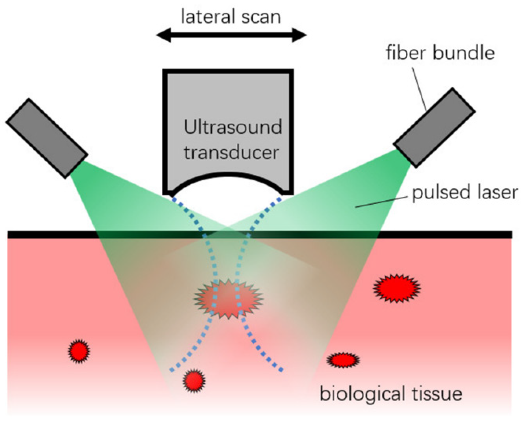
In AR-PAM, it is assumed that the pulsed laser gives homogenous illumination to the biological tissue, and the optical attenuation is not generally considered in the image reconstruction. A focused transducer with high central frequency and high NA scans over the surface of the biological tissue, which detects the ultrasound pulses generated by the thermal expansion due to the absorption of the pulsed laser, as seen in Figure 1.

This assumes a focused transducer scanned over N positions, with a step size of Δx. The detected photoacoustic pressure at an arbitrary point can be expressed with the following Fresnel integral over the transducer surface S [19]:

$$P(t)={\displaystyle {\int }_{S}p(R,t)dS(R)}=\frac{\Gamma }{4\pi v}\frac{\partial }{\partial t}{\displaystyle \underset{S}{\int }dS(R){\displaystyle {\int }_{\Omega }\frac{H(r\text{'})\delta (t-\left|r-r\text{'}\right|/v)}{\left|r-r\text{'}\right|}dr\text{'}}}$$

(1)

Here Γ is the Grüneisen coefficient, a dimensionless constant representing heat conversion efficiency to pressure. The media is assumed to be acoustically homogenous with an acoustic velocity of v. We take that the optical absorption distribution H(r’) in the imaging domain Ω can be expressed as a total of NPs evenly distributed point sources. The transducer surface is also described as a total of NPd evenly distributed point detectors. Then, considering the transducer’s acoustic–electrical response function h^e(t), the integral in Equation (1) is changed to the following convolution function for calculating the received photoacoustic signal of the transducer S(t):

$$\begin{array}{cc}S(t)\hfill & =P(t)\otimes h^e(t)\hfill \\ & ={\displaystyle \sum _{i=1}^{NPd}{\displaystyle \sum _{j=1}^{NPs}\frac{A(r_j)\left[\frac{\partial }{\partial t}\delta (t-\left|R_i-r_j\right|/v)\right]\otimes h^e(t)}{\left|R_i-r_j\right|}}}\hfill \\ & ={\displaystyle \sum _{i=1}^{NPd}{\displaystyle \sum _{j=1}^{NPs}\frac{A(r_j)}{\left|R_i-r_j\right|}\frac{\partial }{\partial t}{h}^e(\left|R_i-r_j\right|/v)}}\hfill \\ & ={\displaystyle \sum _{i=1}^{NPd}{\displaystyle \sum _{j=1}^{NPs}\frac{A(r_j)}{\left|R_i-r_j\right|}{h}^{pf}(\left|R_i-r_j\right|/v)}}\hfill \end{array}$$

(2)

Here h^pf(t) is the system’s point transfer function, R_i donates the i-th point detector’s position, r_j donates the j-th point source’s position, and A(r_j) donates the intensity of the point source. Here the constants are omitted, and the finite nature of the function h^e(t) (both values and derivations of this function at infinity are zeros) is utilized to calculate the convolution. We only need the system’s point transfer function h^pf (t) to calculate the acoustic data if we have the point sources’ positions and intensities. In our simulations, a Gaussian-enveloped cosine function was assumed for this point transfer function, but it can also be experimentally measured with a point source.

2.2. The GPU Parallel Scheme of Data Generation

Because the number of NPd is about several hundred, and NPs can be easily more than one million, the calculation cost of Equation (2) can be prohibitively expensive for CPUs. Thus, we parallelized the summation with GPU to speed up the data generation in a Matlab environment [20] in which a mexCuda function is called to calculate each A-line.

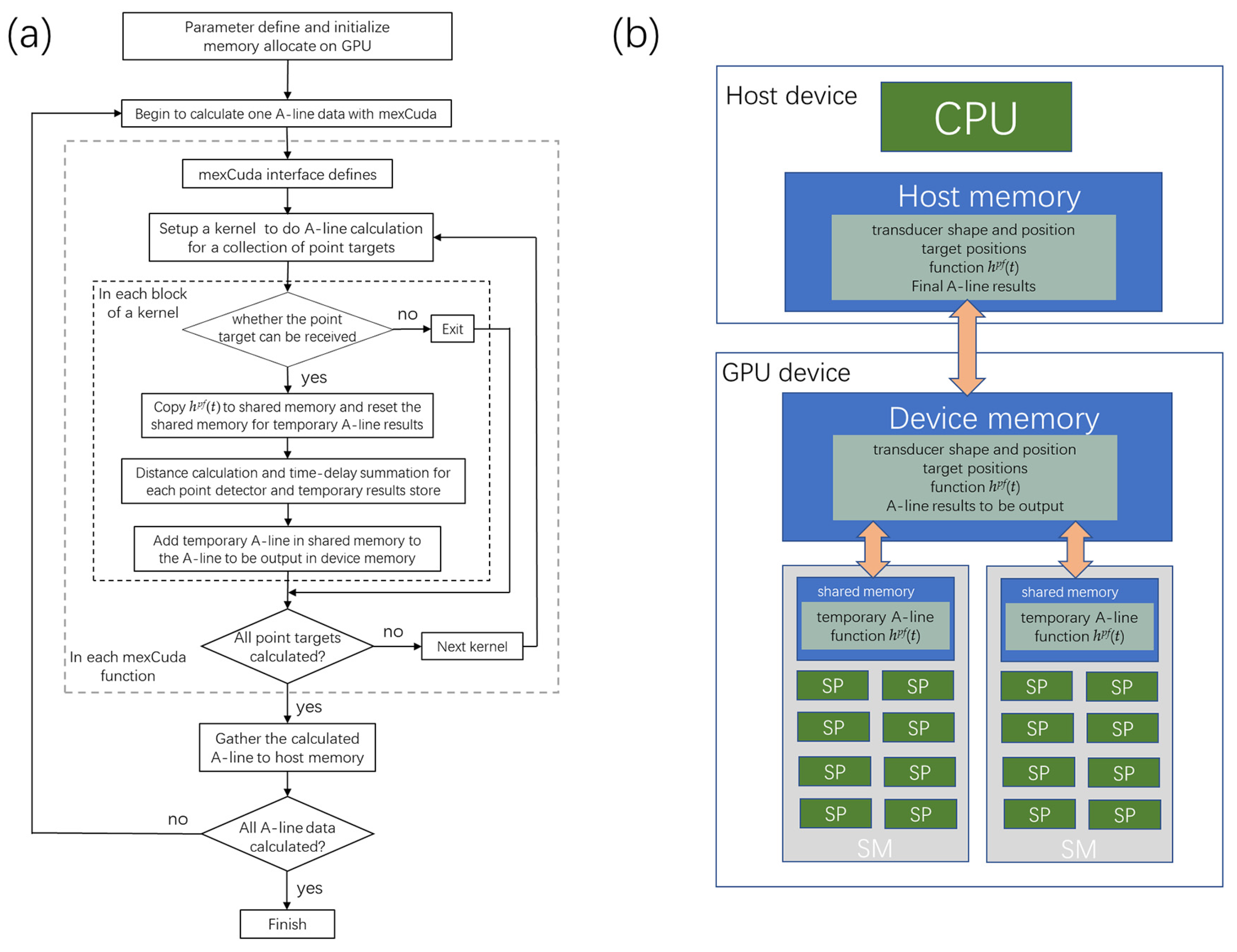
As seen in the flow chart in Figure 2a, after the parameter definition and initialization, input matrixes such as the transducer’s shape and position, target point positions, and the system’s point transfer function were changed into gpuArray, and stored in the device memory in the GPU card, as seen in Figure 2b. The mexCuda function (indicated with gray dotted lines) is programmed in C language, which defines interfaces between the C language and the Matlab language and calculates Equation (2). The mexCuda function is divided into several kernels (indicated with black dotted lines) for the A-line calculation, and each kernel deals with the parallel calculation of several thousand point targets—this kind of design helps to avoid possible kernel computation timeouts.

Each block calculates one point target of the blood vessel network in each kernel, which is calculated in the stream multiprocessor (SM). Each thread in the block deals with each point detector of the transducer, calculated in the stream processor (SP). In each block, the first thread judge whether the transducer can receive the point target. Then the threads copy the system’s point transfer function into the shared memory, calculate the distance from the point target to the point detectors, and compute the corresponding time-delay summing. The summing results in each block were stored in the shared memory. Using the shared memory can significantly improve the data transfer bandwidth and helps to improve the calculation speed. The temporary results for each point target are summed back to the A-line in the device memory, which is finally gathered by the Matlab program. Results show that the mexCuda-based forward data generation is about 300 to 500 times faster than the Matlab-based version.

2.3. The BP-Based Reconstruction Methods

The conventional B-mode photoacoustic image reconstruction is performed by simply back-aligning the acquired A-lines according to the flight time of ultrasound signals so that the resulting pixel value at position (x,y) is taken as the signal intensity of the A-line collected at x at time y/v [1,12]:

$$I(x,y)=S_x(y/v)$$

(3)

Here x donates the lateral position, and y donates the depth position, which is usually set relevant to the center of the detector surface. However, the lateral resolution in the out-of-focus regions is significantly reduced because it assumes that the acoustic beam travels along a thin line, only valid in the transducer’s focal zone.

Therefore, many BP-based algorithms have been proposed which account for the transducer’s detector geometry in a simple, robust, and quick way to restore the elongated lateral resolution. The synthetic-aperture-focusing-technique (SAFT) method assumes the focus of the transducer as a virtual point detector (VPD), then applies time delay relative to the position of VPDs in a circle, and sums the delayed signals with the transducer’s spatial impulse response (SIR) for intensity compensation, which is [12,16,21]:

$$I(x,y)={\displaystyle \sum _{i=1}^{circle}S(x_i,\Delta t(x-x_i,y))·SIR(x-x_i,y)}$$

(4)

Here the time delay Δt and the SIR are functions of the relative lateral position of the summed A-line x−x_i and the depth position of the pixel y. The synthesized aperture size of the circle is equivalent to the NA of the transducer. This Equation can be multiplied with a coherent factor (CF) to further improve the resolution by suppressing the side lobes, which is the SAFT-CF method [13,16,21]:

$$\begin{array}{cc}I(x,y)& =I_{SAFT}(x,y)·CF(x,y)\hfill \\ & =I_{SAFT}(x,y)\frac{{\left|{\displaystyle \sum _{i=1}^{circle}S(x_i,\Delta t(x-x_i,y))·SIR(x-x_i,y)}\right|}^2}{N{\displaystyle \sum _{i=1}^{circle}{\left|S(x_i,\Delta t(x-x_i,y))·SIR(x-x_i,y)\right|}^2}}\hfill \end{array}$$

(5)

Here the N is the number of synthesized A-lines, and the range of the CF weighting factor is from 0 to 1. It is noted that the summation in SAFT is performed within the NA of the transducer. To enable the summing out of the NA for code implementation simplicity, many other algorithms have been proposed recently, and the spatial–temporal response (STR)-based back-projection method (STR-BP) is one such method, which is [19]:

$$I(x,y)={\displaystyle \sum _{i=1}^{N}S(x_i,\Delta t_{STR}(x-x_i,y))·w_{STR}(x-x_i,y)}$$

(6)

where N is the total number of transducer positions and Δt_STR and w_STR are the time delay and weighting coefficient acquired with the STR of the transducer. The improved back-projection (IBP) method is another commonly used method that accounts for the geometry of the transducer detection surface, which can also be performed out of the NA of the transducer [17]. It assumes that the transducer detection surface is composed of a collection of point detectors and is given as:

$$I(x,y)={\displaystyle \sum _{i=1}^N{\displaystyle \sum _{j=1}^{NPd}S(x_i,\Delta t(x-x_{ij},y-y_{ij}))}}$$

(7)

Here the time delay Δt is calculated as the flight time from the pixel to the point detector. The signal from the whole transducer approximates the signal of all the point detectors.

2.4. Experiment Design

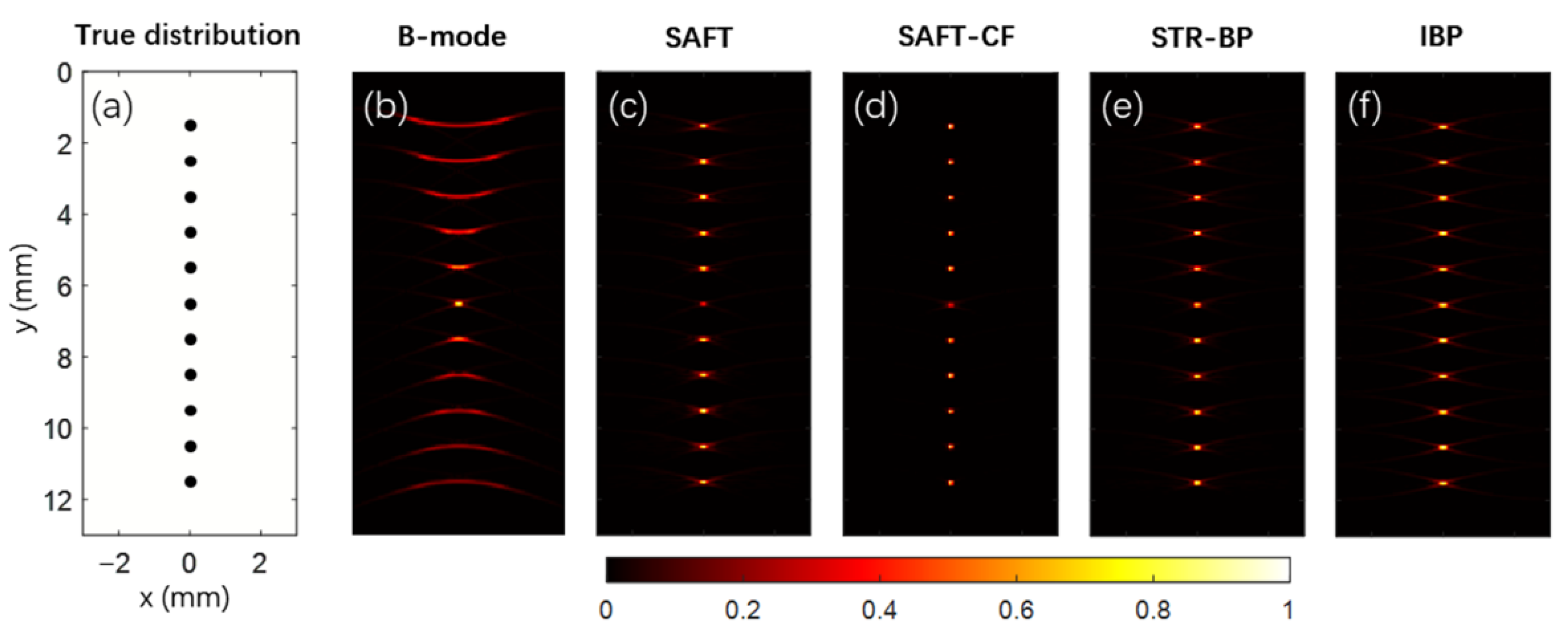
This research performed numerical simulations for point targets and complicated blood vessel networks. A focused transducer with 20 MHz central frequency and 80% bandwidth was employed in these simulations. The aperture size of the transducer was 6 mm, its focal length was 10 mm, and the focus was set at a depth of 6.5 mm. There were 301 transducer positions evenly distributed within a scanning range of 15 mm in the lateral direction. The origin of the coordinates was set at the center of the top boundary of the image domain, and the transducer detection surface was 3.5 mm above the image domain. The above are the default simulation parameters unless otherwise noted. The simulated data was applied with Hilbert transform, and the module of the complex pixel value was taken as the reconstruction results. Photoacoustic images reconstructed with the conventional B-mode method, the SAFT method, the SAFT-CF method, the STR-BP method, and the IBP method are compared. A total of 11 points were evenly distributed along the depth direction in the point target simulations, with a 1 mm interval. For resolution comparison, we take the full width at half-maximum (FWHM) of the lateral profile of the point target as its lateral resolution. 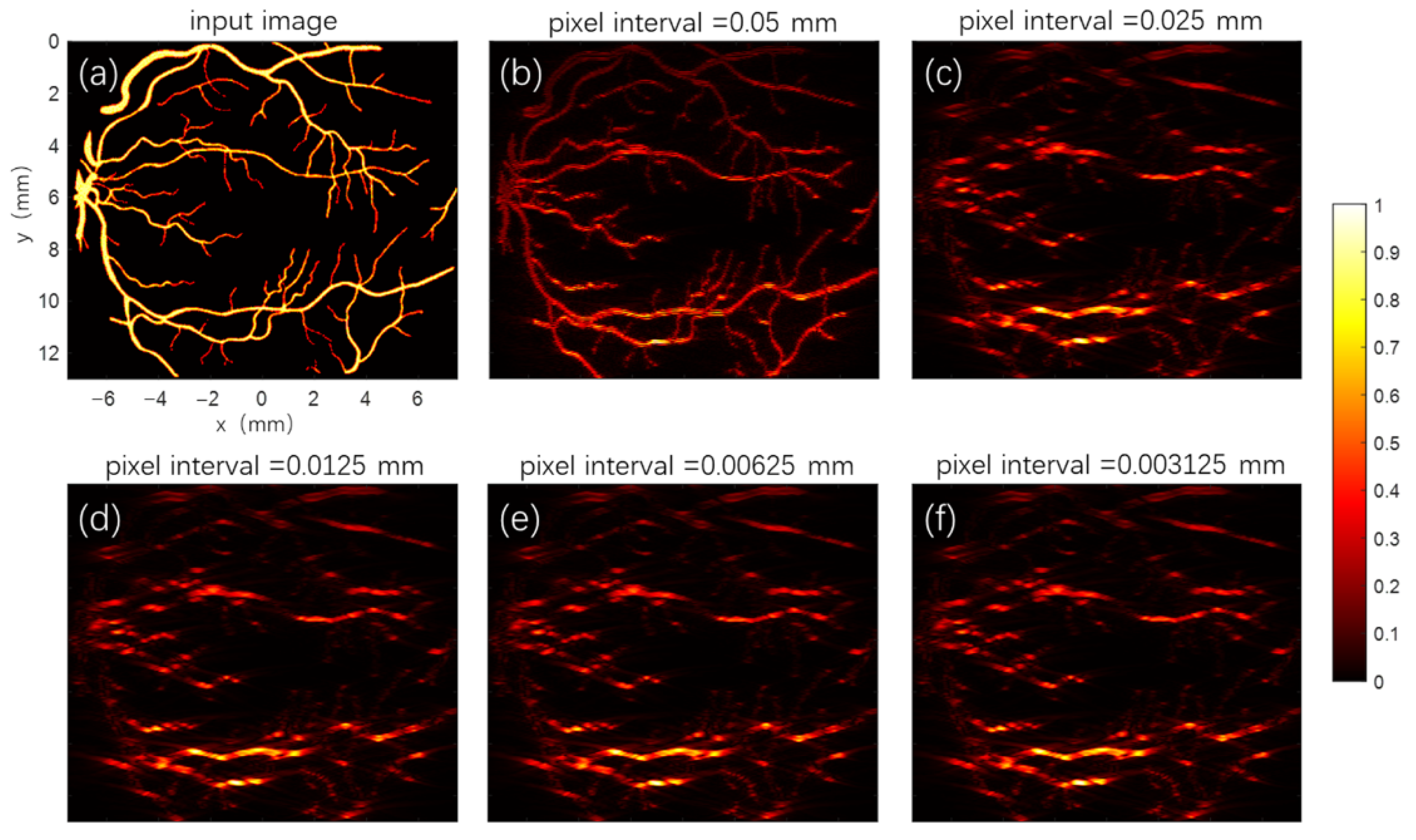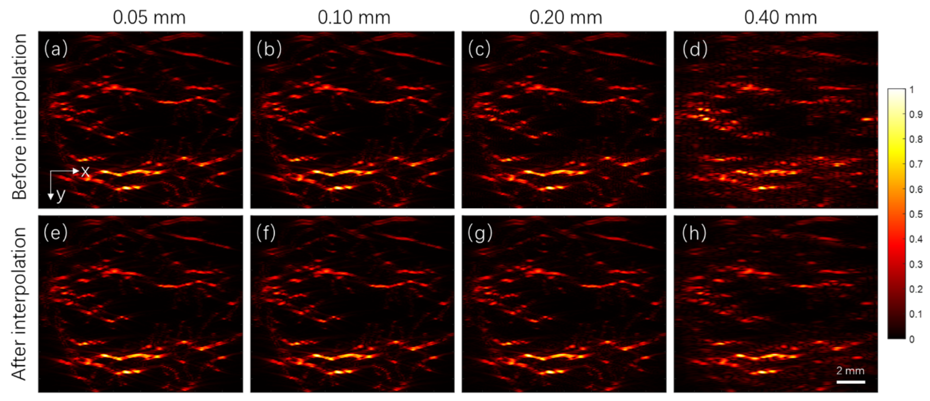For the stability test, an ensemble-based method was applied to calculate the signal-to-noise ratio (SNR) at the point target positions for each algorithm, with 5% Gaussian white noise added [22]. A complex digital blood vessel network was employed in the blood vessel network imaging. We studied the setting parameter of point density required in the simulation and compared the reconstructed images with these algorithms. We compared the results reconstructed with different numbers of A-lines. In the case of a small number of A-lines, we interpolated the data for more input numbers of A-lines and compared the results before the data interpolation. We also compared the reconstruction results under different noise levels to see the improvement in peak signal-to-noise ratio (PSNR) using the STR-BP method compared with the conventional B-mode method.

3. Results

3.1. Point Targets Simulations

Figure 3a shows the actual distribution of the point target and Figure 3b–f are the reconstructed images with the abovementioned five methods. In the conventional B-mode method, only the point target at the transducer focus has the optimal lateral resolution (in the x-axial direction). With the other four reconstruction methods, the lateral resolution out of the focal regions is almost entirely restored by accounting for the geometry of the transducer’s detection surface. In this work, all the maximum value of each photoacoustic image was normalized to 1, and the color bar indicates the normalized photoacoustic intensities of the pixels in arbitrary units, otherwise noted.

We extracted the change of lateral resolution, SNR, and relative amplitude with the target depth for each reconstruction method for further analysis. As seen in Figure 4a, the elongated lateral resolution of the B-mode method is well restored in the other four methods. Figure 4b is a zoomed image of Figure 4a, and it is seen that there are slight differences in the lateral resolution among the four back-projection-based methods. The SAFT-CF method has the best lateral resolution because it significantly depresses the side lobes using the CF coefficients. The B-mode, SAFT, and SAFT-CF methods have a similar lateral resolution at the transducer focus because they have the same formula at the transducer focus. For the STR-BP and IBP methods, their lateral resolution is relatively higher. The lateral resolutions by the SAFT, the STR-BP, and the IBP methods are near for the out-of-focus regions. However, because the CF coefficient is non-linear and noise sensitive, the SNR of the SAFT-CF method is lower than the SAFT, STR-BP, and IBP methods in the out-of-focus regions, as seen in Figure 4c.

Nevertheless, the four back-projection-based methods give much higher SNR than the conventional B-mode method in the out-of-focus regions. Figure 4d shows each method’s relative target amplitude reconstructed. It is seen that the target intensity at the transducer focus given by the SAFT and SAFT-CF is significantly lower than the out-of-focus regions because these two methods are only approximate methods, and the acoustic field of the focused transducer is not well modeled in these two methods. Comparatively, the STR-BP method employs a pre-calculated field map of the transducer. In the IBP method, the acoustic field of the transducer is inherently considered (although with a much higher computational cost). Thus, the reconstructed target intensity by the two methods is more consistent.

3.2. Determining the Density of Point Sources

Figure 5a is the input image of the complex blood vessel network for the simulations. Figure 5b is the reconstruction results of the STR-BP method, with a pixel interval of 0.05 mm for the input image. Here we choose the STR-BP method because it can balance the computational cost, SNR, and consistency of target intensity quite well. In Figure 5b, the whole blood vessel network is well reconstructed. However, as the pixel interval becomes 2, 4, 8, and 16 times smaller (for Figure 5c–f, respectively) only the blood vessels that are parallel to the lateral direction can be reliably reconstructed. A smaller pixel interval means more point sources are considered in the forward data generation with Equation (2). The blood vessel is more like a continuous target than a collection of isolated point sources. These results are consistent with the knowledge that only the oblique features of the transducer axis can be well detected. As the pixel interval is smaller than 0.025 mm, there is little difference in the reconstructed images. As seen in Figure 4b, the lateral resolution for the SAFT-CF method is around 0.1 mm and about 0.15 mm for the other three BP-based methods. This means that the pixel interval of the input image should be at least 4 to 6 times smaller. In this work, we chose a pixel interval of 0.0125 mm for the input image for insurance purposes.

3.3. Reconstruction Results with Different Methods

Figure 6 shows the reconstruction results given by different methods. As seen in Figure 6b, in the conventional B-mode algorithm, the image is seriously blurred in the lateral direction in the out-of-focal regions (focus at y = 6.5 mm). In contrast, this blur is well reduced in the other four methods. It is also noticed that there are more isolated points in the SAFT-CF method than the other reconstructed images, which proved that the SAFT-CF is more effective for point targets. It is also noticed that the mean signal intensity in the images with STR-BP and IBP is notably higher near the transducer focus than in the images by the SAFT and SAFT-CF method, as indicated with dotted white ellipses, which is consistent with the results in Figure 3d.

3.4. Image Reconstruction with a Small Number of A-Lines

Figure 7a–d show the reconstructed images by the STR-BP method when the step size was 0.05 mm, 0.1 mm, 0.2 mm, and 0.4 mm, respectively. It is seen that as the results in Figure 7a–c are similar, but Figure 7d is notably blurred in the lateral direction. This means that the step size of the lateral scan should be smaller than 0.4 mm to ensure the quality of the reconstructed image. Figure 7e–h shows the corresponding results to Figure 7a–d when the forward photoacoustic data was interpolated to keep a step size of 0.05 mm. However, we see that the results in Figure 7f–h are similar to those in Figure 7b–d. This indicates that data from a few A-lines cannot be interpolated to produce more A-lines to restore the lost information.

3.5. Reconstruction Results in Different Noise Levels

Figure 8a–d shows the reconstructed images by the conventional B-mode method and the STR-BP method when the noise level varied from 5% to 25%. The Gaussian white noise was generated with the Box–Muller method, and the noise level is defined as the noise’s standard deviation to the noise-free data’s maximum amplitude. As seen from Figure 8a–d, when the noise increases, the image quality dramatically deteriorates for the B-mode method. At each noise level, the image quality given by the STR-BP method (Figure 8e–h) is much higher than the B-mode method. For quantitative assessment, we chose a square background region of 2.25 mm² near the center of the image, obtained its standard deviation for pixel intensity as the image noise level, and calculated the PSNR of the image. Results showed that the PSNRs were 31.9 dB, 25.5 dB, 22.1 dB, and 18.8 dB for the noise level of 5%, 10%, 15%, and 25%, respectively, with the B-mode method. Comparatively, the corresponding PSNRs were 39.4 dB, 32.2 dB, 29.1 dB, and 23.6 dB, respectively, with the STR-BP method. Thus, the STR-BP method shows a 4.7 to 7.5 dB improvement in the PSNR. It is also noted that while few structures are seen in Figure 8d, the STR-BP method helps the image withstand a noise level of 25% so that many blood vessel structures remain in Figure 8h. Both the reconstructed images and the quantitative results of PSNR indicate that the BP-based algorithms help reveal more delicate features than the conventional B-mode method by directly improving the PSNR of the image.

4. Discussion

High-quality vascular imaging is crucial to the accurate diagnosis of cancers by AR-PAM. Compared with in vivo experiments, numerical simulation provides a low-cost and convenient means to characterize AR-PAM performance for vascular imaging. Through the in-depth simulation studies, we can find ways to optimize the scanning and image reconstruction of AR-PAM. On the other hand, there are debates about applying the SAFT-based methods in AR-PAM. Some researchers indicated that the SAFT-based techniques are only suitable for point-target imaging [14,18]. Some researchers think that although the CF coefficients can further improve the lateral resolution, they also induce noise amplification [18]. Some researchers have declared that the imaging results with these SAFT-based methods for targets near the transducer focus are not as good as those reconstructed by the conventional B-mode method [15,16]. These remaining issues require intensive and systematic simulation studies.

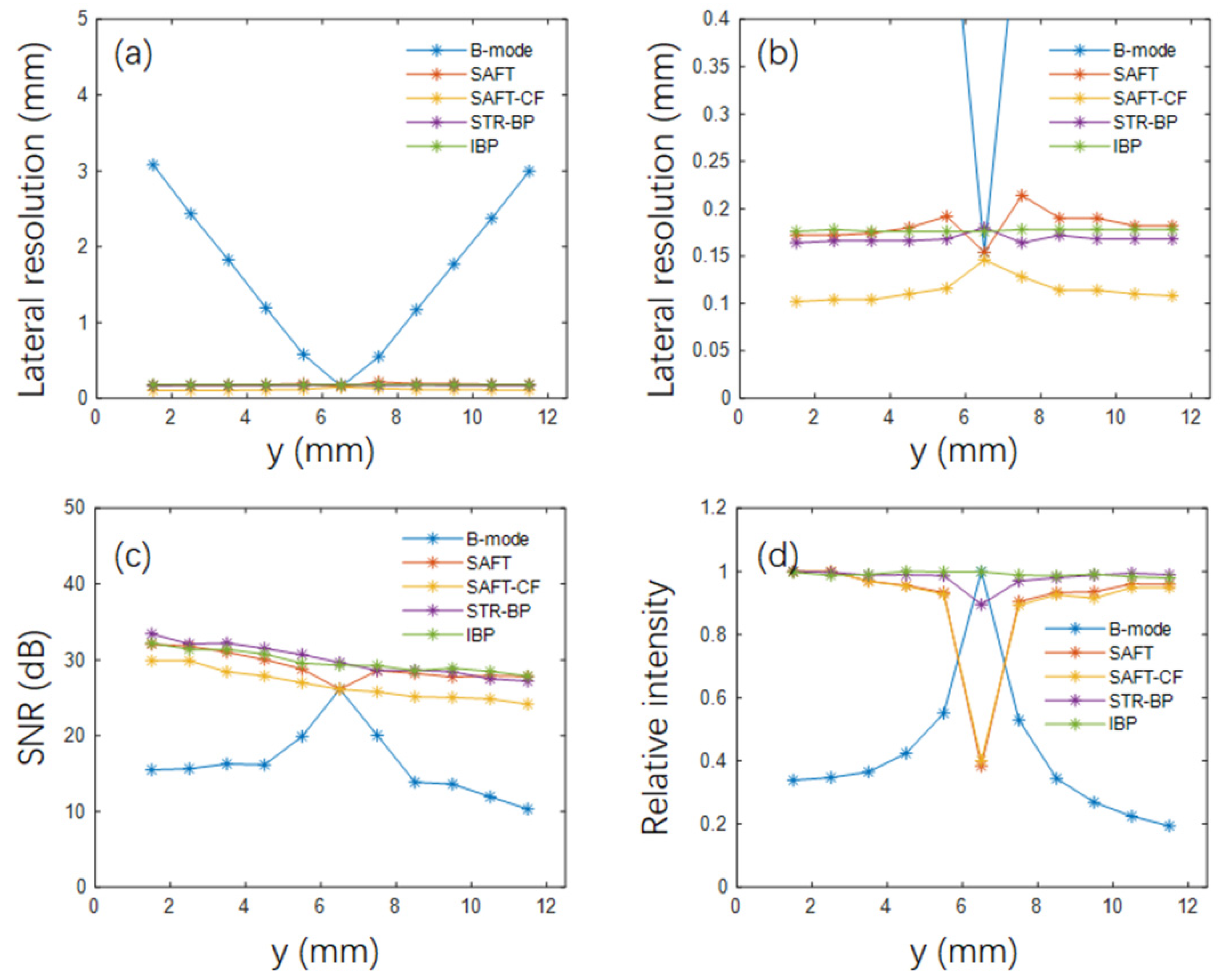
In this work, we set up a framework for generating photoacoustic signals of complicated objects and explored the potential and adaptability of different variations of BP-based methods in imaging complex vascular networks. In the point target simulation, we found that various BP-based advantages in lateral resolution, SNR, and signal intensity consistency. For example, the SAFT-CF method has the highest lateral resolution (about 0.1 mm, compared with about 0.15 mm for the other three BP-based methods). Still, its SNR is generally 2–3 dB lower because the nonlinear CF coefficient is sensitive to noise. The IBP method has the best signal intensity consistency because it inherently considers the acoustic field of the transducer by dividing the transducer aperture into small point detectors, but it significantly increases its computation cost.

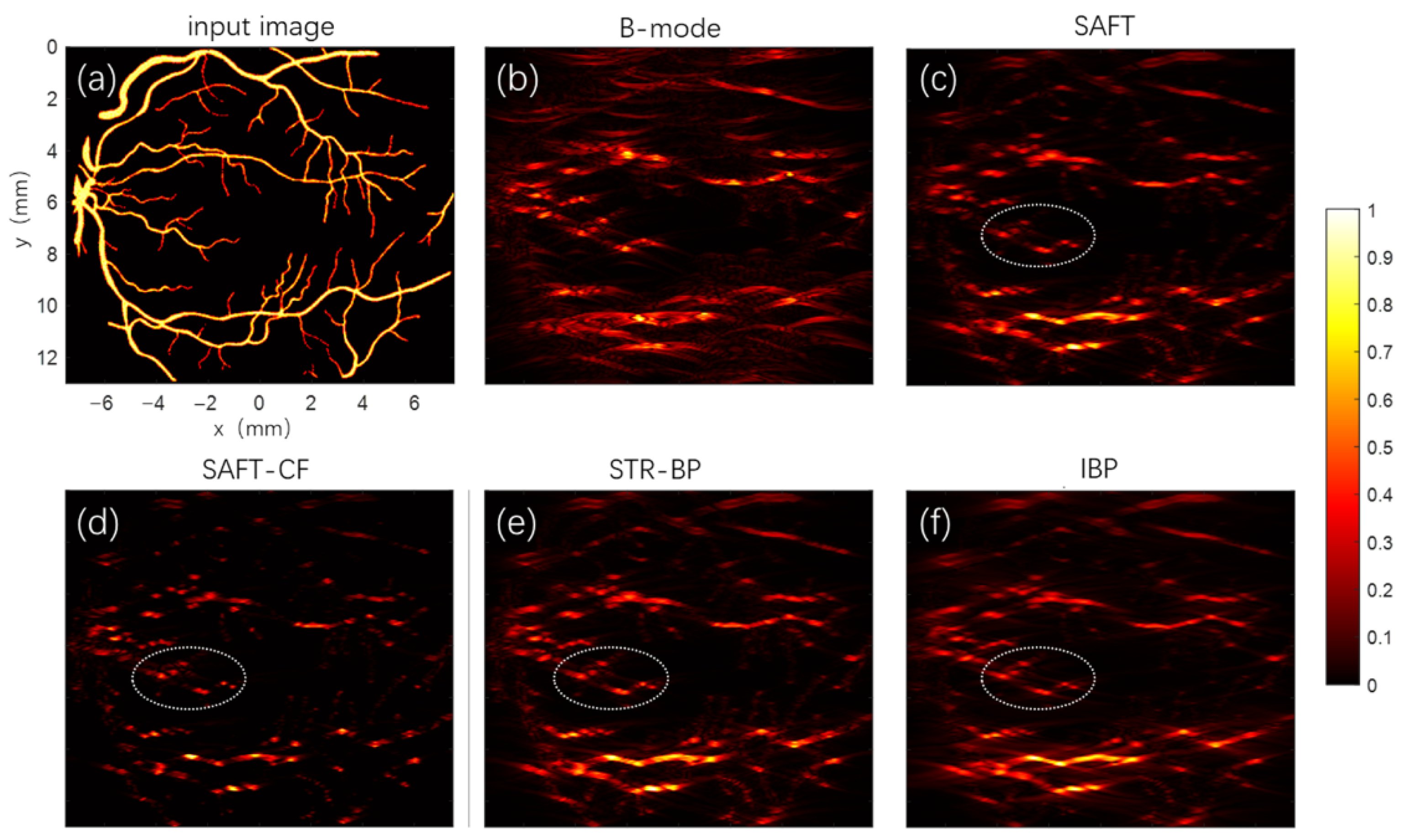
In current studies, the SAFT-CF method is mainly employed to improve the lateral resolution in the out-of-focus regions. However, its advantage is primarily demonstrated with point targets such as the cross-section of blood vessels. The blood vessel simulation in this work revealed that the proposed four BP methods improved the image quality in the off-focal regions. It is noted that three out of the four methods showed slightly different results since they are all based on the modeling of the acoustic field of the transducer, except for the SAFT-CF method, which is more effective for point targets. Although CF coefficients help to improve the lateral resolution of point targets (as seen in Figure 3b), they are sensitive to data noise (as seen in Figure 3c) and degrade the reconstructed image quality of the vascular networks (as seen in Figure 5d). Thus, the SAFT-CF method is not recommended in continuous blood vessel imaging. Therefore, we suggest choosing the STR-BP method because it can balance computational cost, SNR, and consistency of target intensity.

In actual experiments, we speculate which of the three reconstruction methods (the SAFT, STR-BP, and IBP) gives better results is only decided by which method models the acoustic field better. Because there are too many factors in the actual experiments, we must probably preprocess the data carefully and try each method before concluding. Although OR-PAM is frequently employed for skin vascular imaging, it cannot fully utilize the high-penetration advantage of PAI. Comparatively, AR-PAM with high-frequency and high NA is more preferred for vascular imaging due to the extended depth. The simulation shows that with the 20 MHz focused transducer, a lateral resolution of about 0.15 mm and an axial resolution of about 0.05 mm can be achieved. Results also show that the BP-based method can withstand a noise level higher than 25%. The noise level and sensitivity of the system drop fast with the increase of the penetration depth due to the strong optical scattering. Considering the spatial restraints of the AR-PAM system and the penetration depth of the commonly used 532 nm high-repetition pulsed laser, we expect that all the arteries and veins in the lateral direction within a depth of 5 mm can be visualized based on our experiences. AR-PAM gives better images of the blood vessels in the depth range of 1 to 5 mm. It is difficult to see the individual arterioles and venules due to the small diameters (generally smaller than 30 μm) [23]. There have already been many studies of imaging the deep-seated subcutaneous blood vessels with AR-PAM [8,10,24,25].

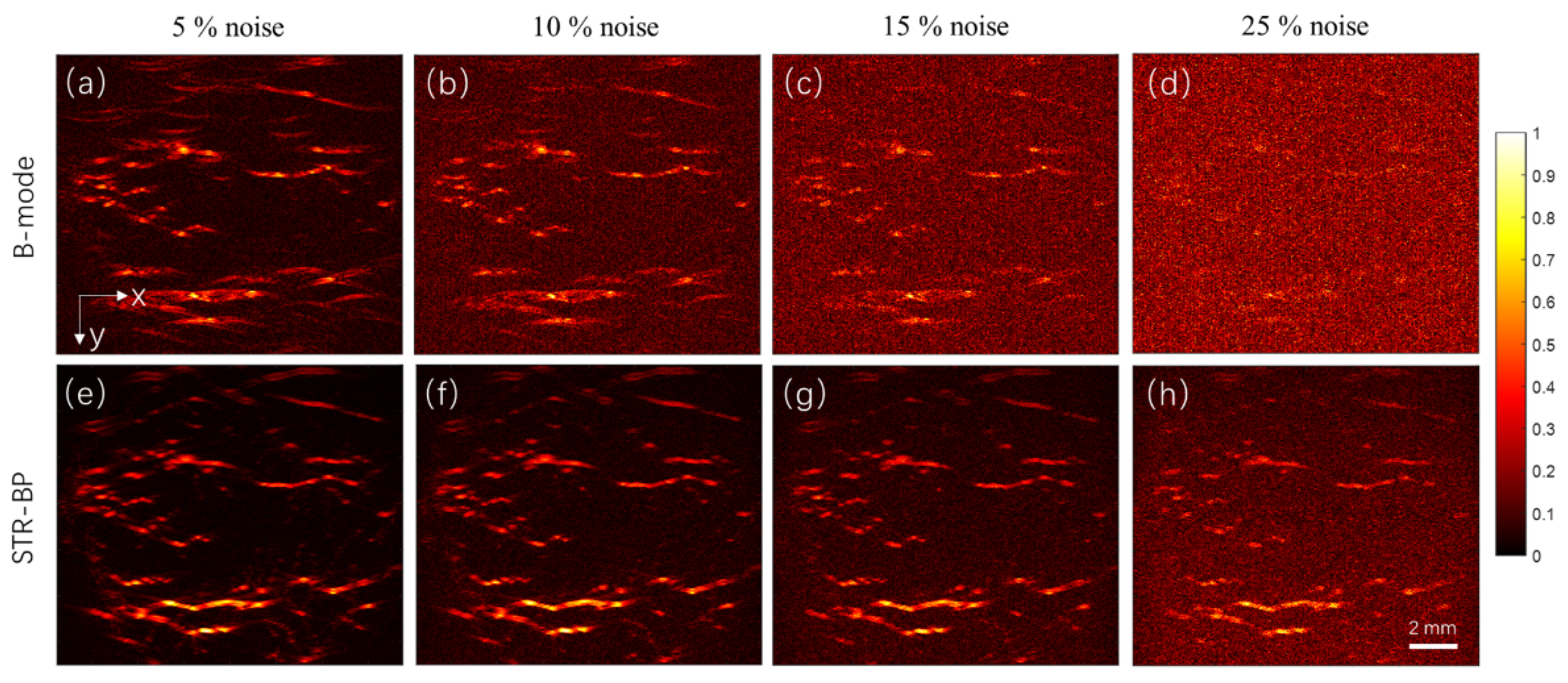
Another important conclusion we have drawn is that data interpolation does not improve image quality. Thus, we infer that the image quality degradation is not due to the back-projection artifacts but may be due to the lost information due to the small detector numbers. Another finding is that the image degradation exists both around the transducer focus and in the out-of-focus regions, as seen in Figure 6d,h, but is most notable around the transducer focus. This is because the sound fields of different A-lines overlap in the off-focal regions, so the information can be complementary.

As a preliminary simulation study of AR-PAM in vascular imaging, some shortcomings need to be overcome in the studies that follow. Firstly, only the data generation was paralleled with GPU in this work. In future results, we will also parallel the image reconstruction. Secondly, the vascular network mainly consists of line targets. We will use images containing point and line targets for simulation in future works. Thirdly, as the vascular networks are in 3D, we will develop 3D simulation and reconstruction frameworks in the future. Lastly, we will perform a more detailed and in-depth analysis of the reconstructed vascular images.

5. Conclusions

This study built a GPU-based framework for simulating AR-PAM signals for imaging vascular networks. On this basis, we compared the reconstruction results by different implementations of BP-based methods. Results confirmed that compared with the conventional B-mode image reconstruction method, the BP algorithms above improve image reconstruction for both point and continuous-line-like complex blood vessels outside of the focal regions. In particular, the SAFT-CF algorithm is more effective for point targets. Comparatively, the STR-BP has higher adaptability and can balance the computational cost, SNR, and consistency of target intensity well. The STR-BP method can improve the PSNR by about 5 to 8 dB compared with the conventional B-mode method, and it helps the image withstand a noise level of up to 25%. Results also showed that a sufficient small scanning step size is required to ensure the image quality, and simply interpolating the data for small detector intervals does not improve the quality of the images. The proposed simulation framework and the findings will guide the design of AR-PAM systems and the choice of appropriate image reconstruction methods.

References

1. Wang, L.V.; Hu, S. Photoacoustic Tomography: In Vivo Imaging from Organelles to Organs. Science 2012, 335, 1458–1462. [Google Scholar] [CrossRef] [PubMed] [Green Version]
2. Fu, Q.; Zhu, R.; Song, J.; Yang, H.; Chen, X. Photoacoustic Imaging: Contrast Agents and Their Biomedical Applications. Adv. Mater. 2019, 31, 31. [Google Scholar] [CrossRef] [PubMed]
3. Weidner, N.; Semple, J.P.; Welch, W.R.; Folkman, J. Tumor angiogenesis and metastasis—Correlation in invasive breast carcinoma. N. Engl. J. Med. 1991, 324, 1–8. [Google Scholar] [CrossRef]
4. Lin, L.; Hu, P.; Shi, J.; Appleton, C.M.; Maslov, K.; Li, L.; Zhang, R.; Wang, L.V. Single-breath-hold photoacoustic computed tomography of the breast. Nat. Commun. 2018, 9, 9. [Google Scholar] [CrossRef] [PubMed]
5. Taruttis, A.; Ntziachristos, V. Advances in real-time multispectral optoacoustic imaging and its applications. Nat. Photonics 2015, 9, 219–227. [Google Scholar] [CrossRef]
6. Attia, A.B.E.; Balasundaram, G.; Moothanchery, M.; Dinish, U.S.; Bi, R.; Ntziachristos, V.; Olivo, M. A review of clinical photoacoustic imaging: Current and future trends. Photoacoustics 2019, 16, 18. [Google Scholar] [CrossRef] [PubMed]
7. Jeon, S.; Kim, J.; Lee, D.; Baik, J.W.; Kim, C. Review on practical photoacoustic microscopy. Photoacoustics 2019, 15, 16. [Google Scholar] [CrossRef]
8. Wang, C.; Guo, L.; Wang, G.; Ye, T.; Wang, B.; Xiao, J.; Liu, X. In-vivo imaging of melanoma with simultaneous dual-wavelength acoustic-resolution-based photoacoustic/ultrasound microscopy. Appl. Opt. 2021, 60, 3772–3778. [Google Scholar] [CrossRef]
9. Hu, S.; Wang, L.V. Neurovascular photoacoustic tomography. Front. Neuroenerg. 2010, 2, 10. [Google Scholar] [CrossRef] [Green Version]
10. Omar, M.; Gateau, J.; Ntziachristos, V. Raster-scan optoacoustic mesoscopy in the 25–125 MHz range. Opt. Lett. 2013, 38, 2472–2474. [Google Scholar] [CrossRef]
11. Caballero, M.A.A.; Rosenthal, A.; Gateau, J.; Razansky, D.; Ntziachristos, V. Model-based optoacoustic imaging using focused detector scanning. Opt. Lett. 2012, 37, 4080–4082. [Google Scholar] [CrossRef] [PubMed]
12. Li, M.; Zhang, H.; Maslov, K.; Stoica, G.; Wang, L.V. Improved in vivo photoacoustic microscopy based on a virtual-detector concept. Opt. Lett. 2006, 31, 474–476. [Google Scholar] [CrossRef] [PubMed] [Green Version]
13. Deng, Z.; Yang, X.; Gong, H.; Luo, Q. Two-dimensional synthetic-aperture focusing technique in photoacoustic microscopy. J. Appl. Phys. 2011, 109, 6. [Google Scholar] [CrossRef]
14. Deng, Z.; Yang, X.; Gong, H.; Luo, Q. Adaptive synthetic-aperture focusing technique for microvasculature imaging using photoacoustic microscopy. Opt. Express 2012, 20, 7555–7563. [Google Scholar] [CrossRef] [PubMed]
15. Turner, J.; Estrada, H.; Kneipp, M.; Razansky, D. Improved optoacoustic microscopy through three-dimensional spatial impulse response synthetic aperture focusing technique. Opt. Lett. 2014, 39, 3390–3393. [Google Scholar] [CrossRef] [PubMed]
16. Cai, D.; Li, Z.; Chen, S. In vivo deconvolution acoustic-resolution photoacoustic microscopy in three dimensions. Biomed. Opt. Express 2016, 7, 369–380. [Google Scholar] [CrossRef] [PubMed] [Green Version]
17. Wang, B.; Wei, N.; Peng, K.; Xiao, J. Modified back-projection method in acoustic resolution-based photoacoustic endoscopy for improved lateral resolution. Med. Phys. 2018, 45, 4430–4438. [Google Scholar] [CrossRef] [PubMed]
18. Jeon, S.; Park, J.; Managuli, R.; Kim, C. A Novel 2-D Synthetic Aperture Focusing Technique for Acoustic-Resolution Photoacoustic Microscopy. IEEE Trans. Med. Imaging 2019, 38, 250–260. [Google Scholar] [CrossRef]
19. Wang, B.; Ye, T.; Wang, G.; Guo, L.; Xiao, J. Approximate back-projection method for improving lateral resolution in circular-scanning-based photoacoustic tomography. Med. Phys. 2021, 48, 3011–3021. [Google Scholar] [CrossRef]
20. Liu, S.; Feng, X.; Gao, F.; Jin, H.; Zhang, R.; Luo, Y.; Zheng, Y. GPU-accelerated two dimensional synthetic aperture focusing for photoacoustic microscopy. APL Photonics 2018, 3, 12. [Google Scholar] [CrossRef]
21. Cai, D.; Li, Z.; Li, Y.; Guo, Z.; Chen, S. Photoacoustic microscopy in vivo using synthetic-aperture focusing technique combined with three-dimensional deconvolution. Opt. Express 2017, 25, 1421–1434. [Google Scholar] [CrossRef] [PubMed]
22. Luo, X.; Xiao, J.; Wang, C.; Wang, B. Fast Correction of “Finite Aperture Effect” in Photoacoustic Tomography Based on Spatial Impulse Response. Photonics 2021, 8, 356. [Google Scholar] [CrossRef]
23. Müller, B.; Lang, S.; Dominietto, M.; Rudin, M.; Schulz, G.; Deyhle, H.; Germann, M.; Pfeiffer, F.; David, C.; Weitkamp, T. High-resolution tomographic imaging of microvessels. In Proceedings of the Developments in X-ray Tomography VI, San Diego, CA, USA, 10–14 August 2008; Volume 7078, p. 70780B. [Google Scholar] [CrossRef] [Green Version]
24. Hu, S.; Wang, L.V. Photoacoustic imaging and characterization of the microvasculature. J. Biomed. Opt. 2010, 15, 011101. [Google Scholar] [CrossRef] [PubMed]
25. Matsumoto, Y.; Asao, Y.; Yoshikawa, A.; Sekiguchi, H.; Takada, M.; Furu, M.; Saito, S.; Kataoka, M.; Abe, H.; Yagi, T.; et al. Label-free photoacoustic imaging of human palmar vessels: A structural morphological analysis. Sci. Rep. 2018, 8, 786. [Google Scholar] [CrossRef] [PubMed] [Green Version]
Figure 1. Schematic of AR-PAM scanning.
Photonics 09 00433 g001
Figure 2. The GPU-based parallel computation scheme for forward data generation. (a) The flowchart of the program and (b) the CPU-GPU parallel architecture, the data storage, and the data flow. SP, stream processor; SM, stream processor.
Photonics 09 00433 g002
Figure 3. Comparison of point targets at different depths reconstructed with different methods. (a) The actual distribution of the point target and (bf) the results given by the B-mode, SAFT, SAFT-CF, STR-BP, and IBP methods, respectively. Here the x-axial is the lateral direction, and the y-axial is the depth direction.
Photonics 09 00433 g003
Figure 4. The comparison of lateral resolution (a,b), SNR (c), and relative intensity (d) given by different reconstruction methods for targets at different depths.
Photonics 09 00433 g004
Figure 5. The reconstructed results of a digital blood vessel network with different pixel intervals of the input image. (a) The input digital blood vessel network and (bf) the reconstruction results given by the STR-BP method when the pixel interval of the input image was 1, 2, 4, 8, 16 times 0.05 mm, respectively.
Photonics 09 00433 g005
Figure 6. The reconstructed results of a digital blood vessel network with different methods. (a) The input digital blood vessel network and (bf) the reconstruction results given by the B-mode, SAFT, SAFT-CF, STR-BP, and IBP methods, respectively.
Photonics 09 00433 g006
Figure 7. The influences of scanning step size and data interpolation on the reconstruction results. (ad) The reconstruction results with the STR-BP method when the step size are 0.05 mm, 0.1 mm, 0.2 mm, and 0.4 mm, respectively, and (eh) the corresponding reconstruction results of (ad) when the forward data is interpolated to keep the step size back to 0.05 mm.
Photonics 09 00433 g007
Figure 8. Reconstructed results of a digital blood vessel network with different central frequencies and NAs of the transducer by the STR-BP method. (ad) The reconstruction results when the central frequencies are 5, 10, 20, and 40 MHz, respectively, and (eh) the reconstruction results when the aperture size of the transducer is 2, 4, 6 and 10 mm, respectively.
Photonics 09 00433 g008
Publisher’s Note: MDPI stays neutral with regard to jurisdictional claims in published maps and institutional affiliations.