A Compressed Reconstruction Network Combining Deep Image Prior and Autoencoding Priors for Single-Pixel Imaging


Abstract
:1. Introduction
- We propose a compressed reconstruction network (DPAP) based on DIP for single-pixel imaging. DPAP is designed as two learning stages, which enables DPAP to focus on statistical information of the image structure at different scales. In order to obtain prior information from the dataset, the measurement matrix is jointly optimized by a network and multiple Autoencoders are trained as regularization terms to be added to the loss function.
- We describe how DPAP optimizes network parameters with an optimized measurement matrix, enforcing network implicit priors. We also demonstrate by simulation that optimization of the measurement matrix can improve the network reconstruction accuracy.
- Extensive simulations and practical experiments demonstrate that the proposed network outperforms existing algorithms. Using the binarized measurement matrix, our designed network can be directly used in single-pixel imaging systems, which we have verified by practical experiments.
2. Related Work and Background
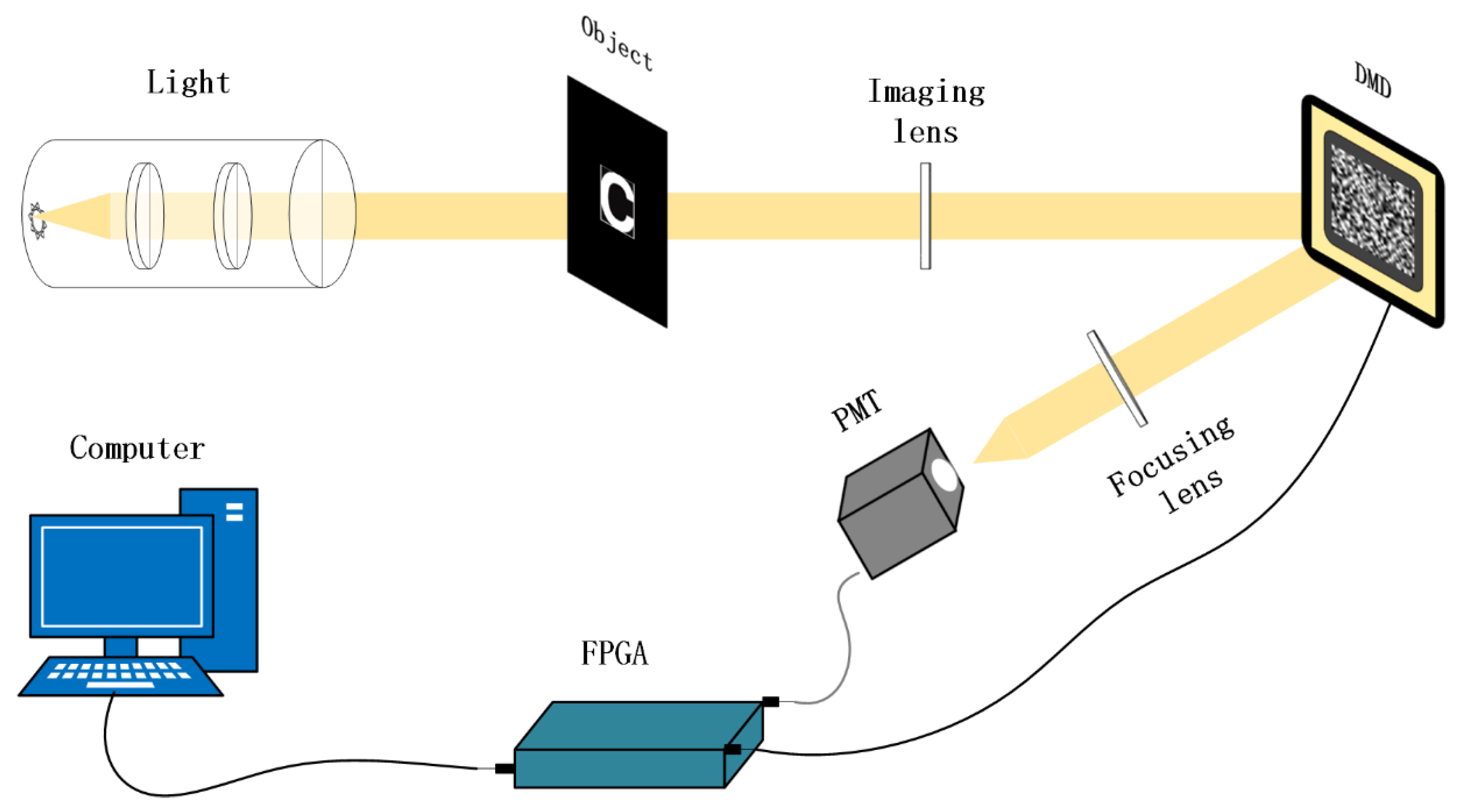
2.1. Single Pixel Imaging System
2.2. Deep-Learning-Based Compressed Sensing Reconstruction Network
2.3. Deep Image Prior
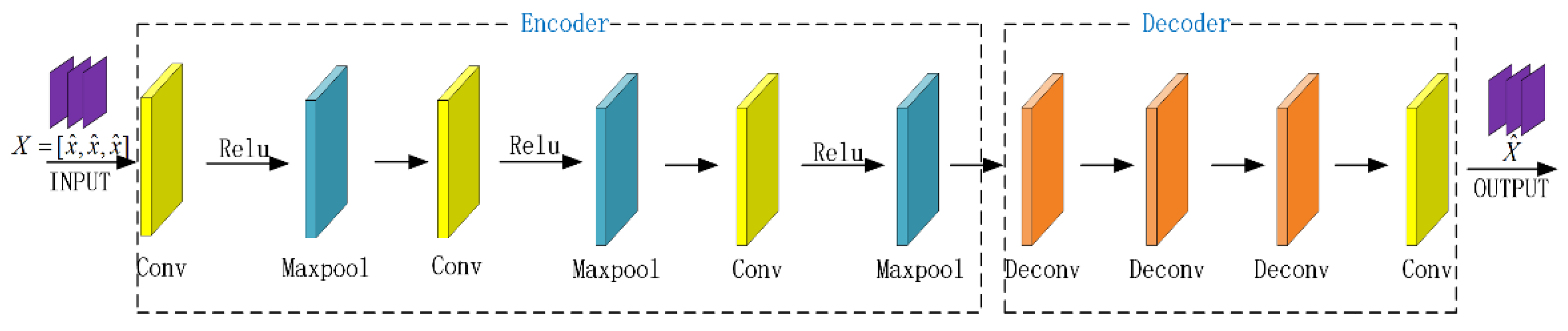
2.4. Denoising Autoencoder Prior
3. Proposed Network
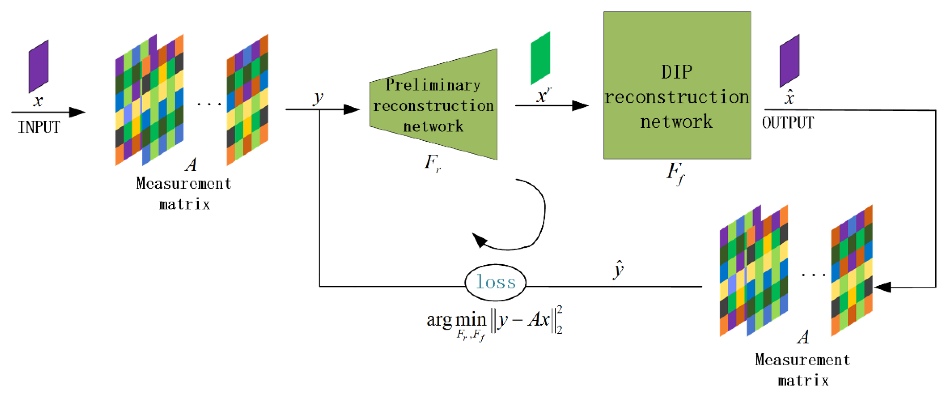
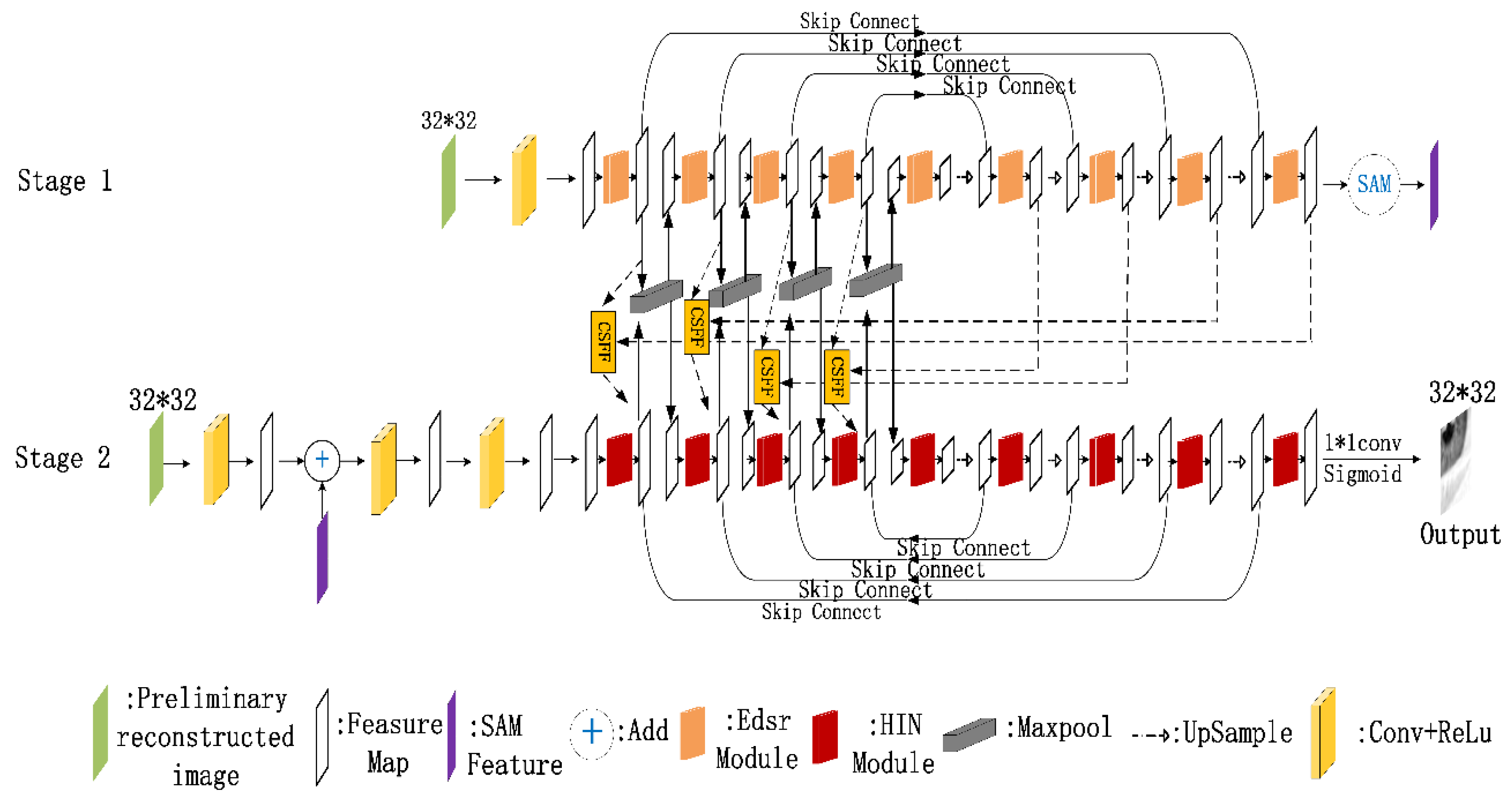
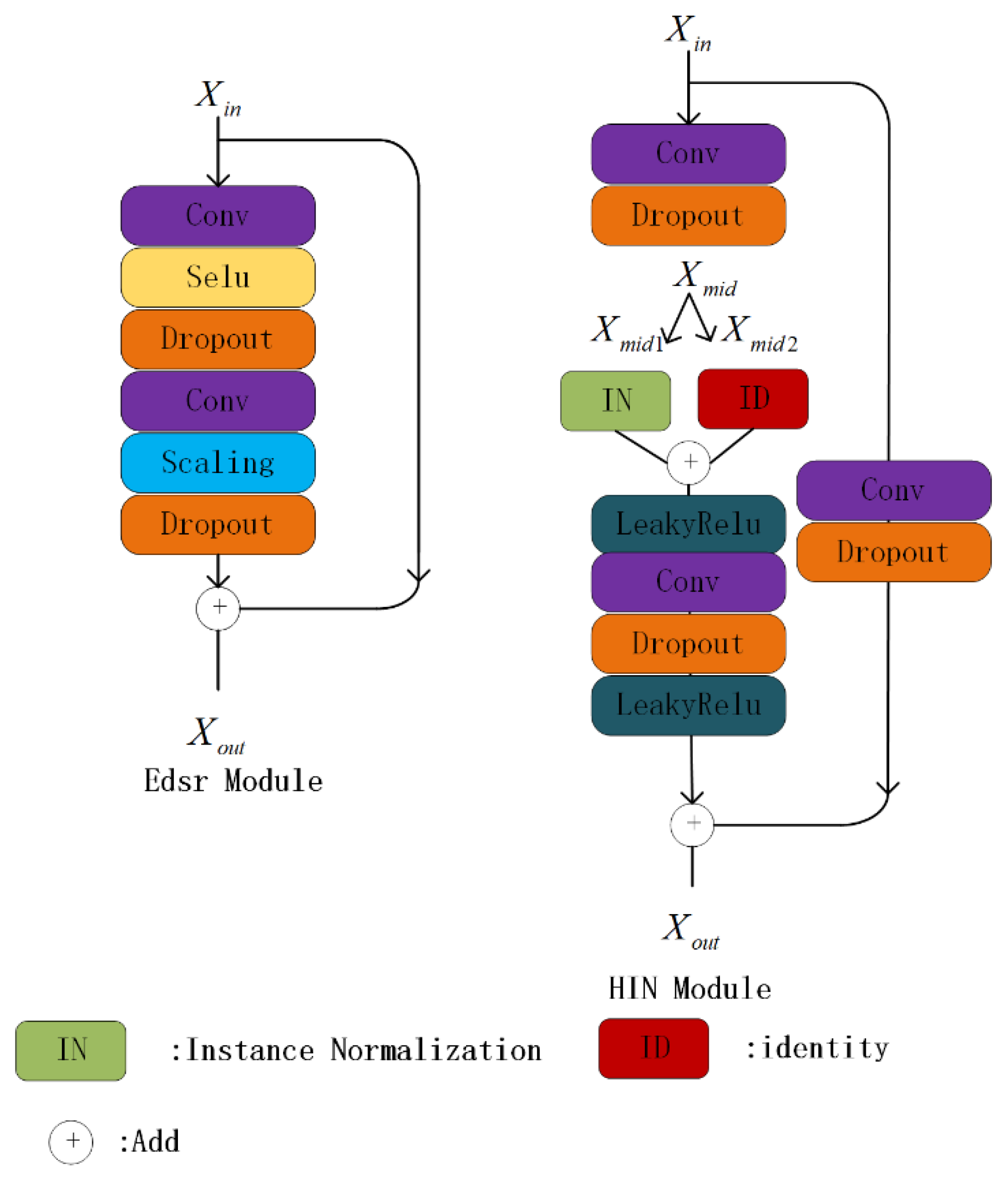
3.1. Network Architecture
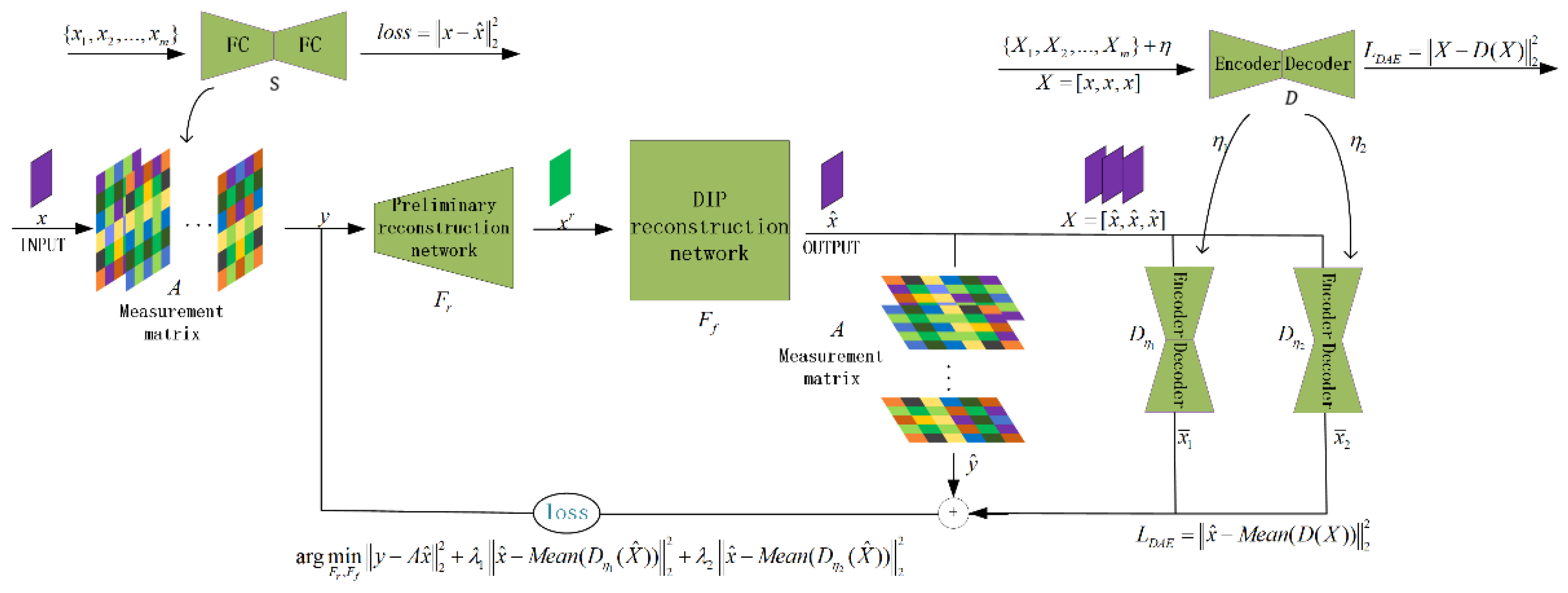
3.2. Loss Function/Regularization Term Design
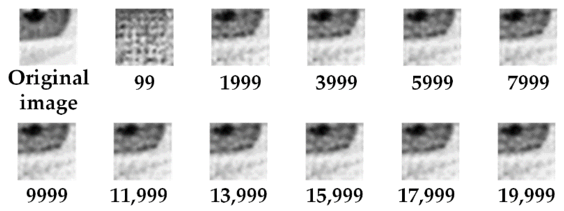
3.3. Training Method
| Algorithm 1 DPAP algorithm |
| Autoencoder training: |
| Initialize encoder weight and decoder weight . |
| For number of training iterations undertake the following: |
| Input batches of data , |
| For all i, Copy the input image as three-channels: |
| Generate Gaussian random noise: |
| Add Gaussian noise: , |
| Compute coded value: |
| Decode the coded value: |
| Updata the and to minimize the reconstruction error: |
| end for |
| Get and . |
| Measurement matrix training: |
| Initializes the weights of the two fully connected layers: . |
| For number of training iterations undertake the following: |
| Input batches of data , |
| For all i, compute the fully connected layer rebuild value: |
| Updata the to minimize the reconstruction error: |
| end for |
| Get and . |
| DPAP testing: |
| Initialize the weight of preliminary reconstruction network and DIP reconstruction network . |
| Restore the fully connected layer weight as the measurement matrix . |
| Restore the Autoencoder weight: and . |
| For number of training iterations undertake the following: |
| Input: just one image |
| Compute measurement value: |
| Compute the value of preliminary reconstruction network and DIP reconstruction network: |
| Compute the measurement value of the reconstruction: |
| Copy the input image as three-channels: |
| Compute Autoencoder error: |
| Compute measurement error: |
| If the Autoencoder error and measurement error are on the same order of magnitude: |
| Updata the preliminary reconstruction network and DIP reconstruction network to minimize reconstruction error: |
| else: |
| Updata the preliminary reconstruction network and DIP reconstruction network to minimize measurement error: |
| end for |
| Return . |
4. Results and Discussion
4.1. DIP Reconstruction Network Performance Verification Experiment
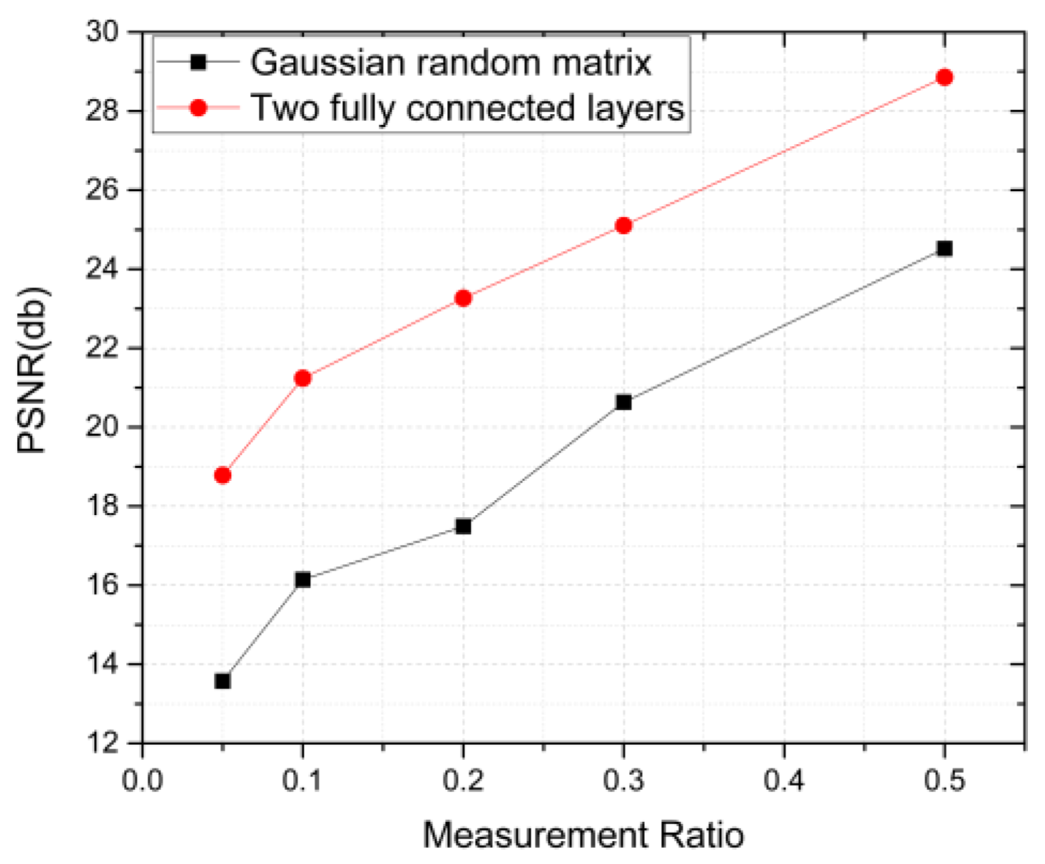
4.2. DPAP Performance Evaluation after Optimizing Measurement Matrix
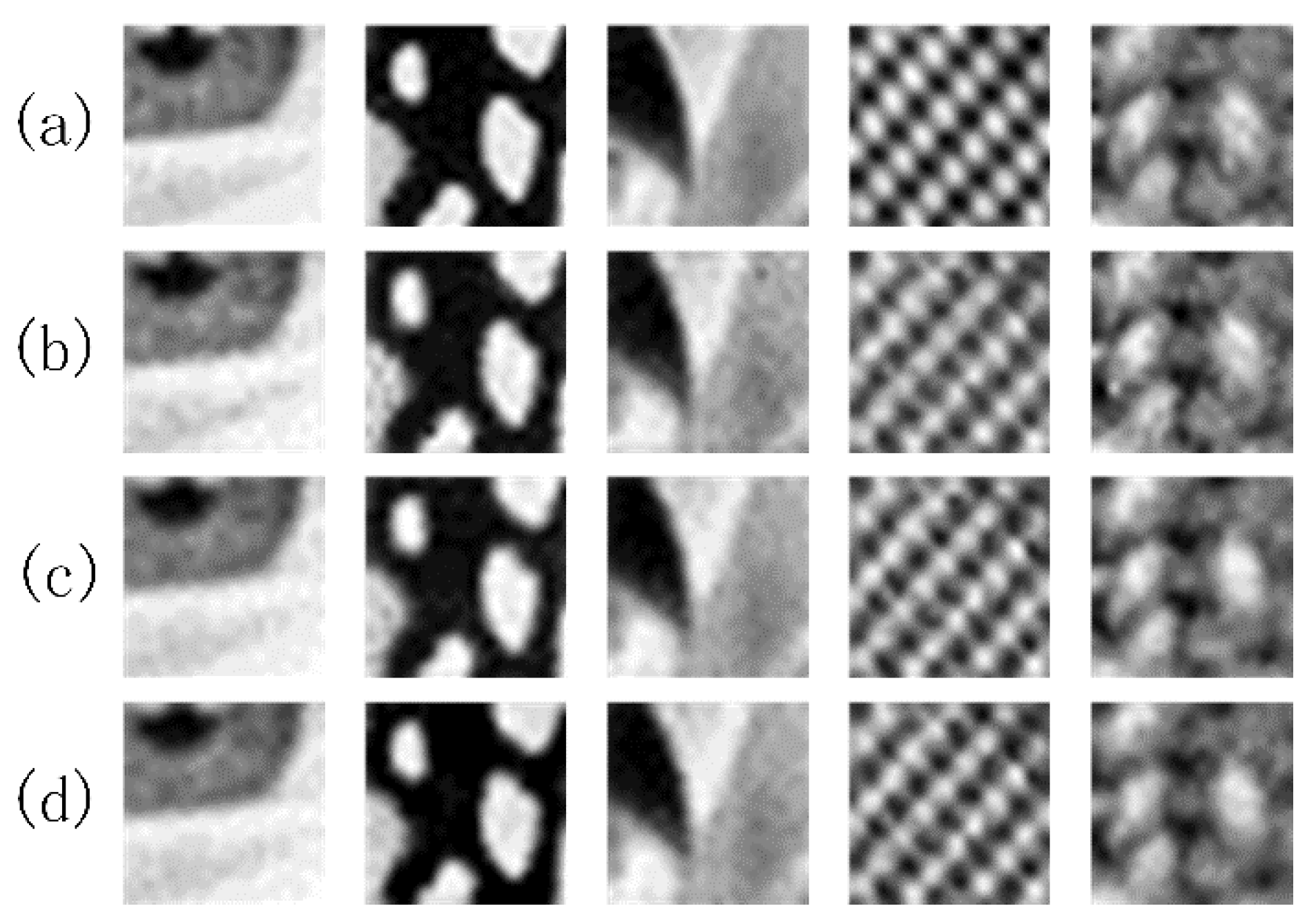
4.3. An Exploratory Experiment on Denoising Autoencoder Priors
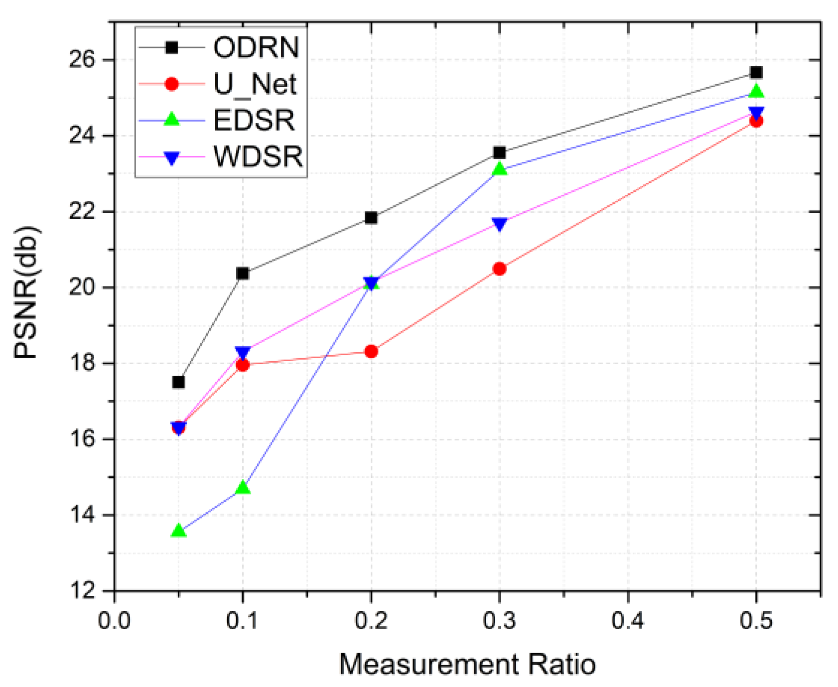
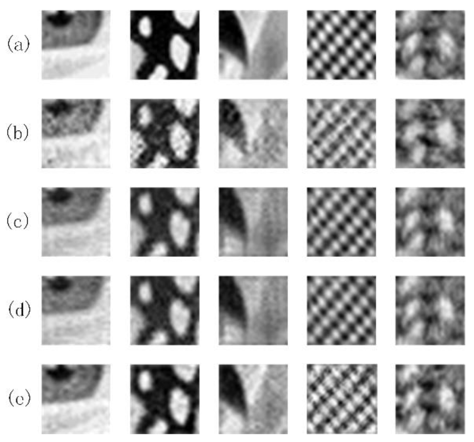
4.4. Comparison of DPAP with Other Existing Networks
4.5. Validation of DPAP on A Single Pixel Imaging System
5. Conclusions
Author Contributions
Funding
Institutional Review Board Statement
Informed Consent Statement
Data Availability Statement
Conflicts of Interest
References
- Studer, V.; Bobin, J.; Chahid, M.; Mousavi, H.S.; Candes, E.; Dahan, M. Compressive fluorescence microscopy for biological and hyperspectral imaging. Proc. Natl. Acad. Sci. USA 2012, 109, E1679–E1687. [Google Scholar] [CrossRef] [PubMed] [Green Version]
- Delogu, P.; Brombal, L.; Di Trapani, V.; Donato, S.; Bottigli, U.; Dreossi, D.; Golosio, B.; Oliva, P.; Rigon, L.; Longo, R. Optimization of the equalization procedure for a single-photon counting CdTe detector used for CT. J. Instrum. 2017, 12, C11014. [Google Scholar] [CrossRef]
- Yu, Y.; Liu, B.; Chen, Z. Improving the performance of pseudo-random single-photon counting ranging lidar. Sensors 2019, 19, 3620. [Google Scholar] [CrossRef] [PubMed] [Green Version]
- Wu, C.; Xing, W.; Feng, Z.; Xia, L. Moving target tracking in marine aerosol environment with single photon lidar system. Opt. Lasers Eng. 2020, 127, 105967. [Google Scholar] [CrossRef]
- Zhou, H.; He, Y.-H.; Lü, C.-L.; You, L.-X.; Li, Z.-H.; Wu, G.; Zhang, W.-J.; Zhang, L.; Liu, X.-Y.; Yang, X.-Y. Photon-counting chirped amplitude modulation lidar system using superconducting nanowire single-photon detector at 1550-nm wavelength. Chin. Phys. B 2018, 27, 018501. [Google Scholar] [CrossRef]
- Liu, Y.; Shi, J.; Zeng, G. Single-photon-counting polarization ghost imaging. Appl. Opt. 2016, 55, 10347–10351. [Google Scholar] [CrossRef]
- Liu, X.-F.; Yu, W.-K.; Yao, X.-R.; Dai, B.; Li, L.-Z.; Wang, C.; Zhai, G.-J. Measurement dimensions compressed spectral imaging with a single point detector. Opt. Commun. 2016, 365, 173–179. [Google Scholar] [CrossRef]
- Jiao, S.; Feng, J.; Gao, Y.; Lei, T.; Xie, Z.; Yuan, X. Optical machine learning with incoherent light and a single-pixel detector. Opt. Lett. 2019, 44, 5186–5189. [Google Scholar] [CrossRef]
- Zuo, Y.; Li, B.; Zhao, Y.; Jiang, Y.; Chen, Y.-C.; Chen, P.; Jo, G.-B.; Liu, J.; Du, S. All-optical neural network with nonlinear activation functions. Optica 2019, 6, 1132–1137. [Google Scholar] [CrossRef]
- Zheng, P.; Dai, Q.; Li, Z.; Ye, Z.; Xiong, J.; Liu, H.-C.; Zheng, G.; Zhang, S. Metasurface-based key for computational imaging encryption. Sci. Adv. 2021, 7, eabg0363. [Google Scholar] [CrossRef]
- Jiao, S.; Feng, J.; Gao, Y.; Lei, T.; Yuan, X. Visual cryptography in single-pixel imaging. Opt. Express 2020, 28, 7301–7313. [Google Scholar] [CrossRef] [PubMed]
- Tropp, J.A.; Gilbert, A.C. Signal recovery from random measurements via orthogonal matching pursuit. IEEE Trans. Inf. Theory 2007, 53, 4655–4666. [Google Scholar] [CrossRef] [Green Version]
- Figueiredo, M.A.; Nowak, R.D.; Wright, S.J. Gradient projection for sparse reconstruction: Application to compressed sensing and other inverse problems. IEEE J. Sel. Top. Signal Processing 2007, 1, 586–597. [Google Scholar] [CrossRef] [Green Version]
- Ji, S.; Xue, Y.; Carin, L. Bayesian compressive sensing. IEEE Trans. Signal Processing 2008, 56, 2346–2356. [Google Scholar] [CrossRef]
- Li, C. An Efficient Algorithm for Total Variation Regularization with Applications to the Single Pixel Camera and Compressive Sensing. Ph.D. Thesis, Rice University, Houston, TX, USA, 2010. [Google Scholar]
- Lyu, M.; Wang, W.; Wang, H.; Wang, H.; Li, G.; Chen, N.; Situ, G. Deep-learning-based ghost imaging. Sci. Rep. 2017, 7, 17865. [Google Scholar] [CrossRef] [PubMed]
- He, Y.; Wang, G.; Dong, G.; Zhu, S.; Chen, H.; Zhang, A.; Xu, Z. Ghost imaging based on deep learning. Sci. Rep. 2018, 8, 6469. [Google Scholar] [CrossRef] [Green Version]
- Higham, C.F.; Murray-Smith, R.; Padgett, M.J.; Edgar, M.P. Deep learning for real-time single-pixel video. Sci. Rep. 2018, 8, 2369. [Google Scholar] [CrossRef] [Green Version]
- Wang, F.; Wang, H.; Wang, H.; Li, G.; Situ, G. Learning from simulation: An end-to-end deep-learning approach for computational ghost imaging. Opt. Express 2019, 27, 25560–25572. [Google Scholar] [CrossRef]
- Wang, F.; Wang, C.; Chen, M.; Gong, W.; Zhang, Y.; Han, S.; Situ, G. Far-field super-resolution ghost imaging with a deep neural network constraint. Light Sci. Appl. 2022, 11, 1–11. [Google Scholar] [CrossRef]
- Zhu, R.; Yu, H.; Tan, Z.; Lu, R.; Han, S.; Huang, Z.; Wang, J. Ghost imaging based on Y-net: A dynamic coding and decoding approach. Opt. Express 2020, 28, 17556–17569. [Google Scholar] [CrossRef]
- Ulyanov, D.; Vedaldi, A.; Lempitsky, V. Deep image prior. In Proceedings of the IEEE conference on computer vision and pattern recognition, Salt Lake, UT, USA, 18–23 June 2018; pp. 9446–9454. [Google Scholar]
- Mousavi, A.; Patel, A.B.; Baraniuk, R.G. A deep learning approach to structured signal recovery. In Proceedings of the 2015 53rd annual allerton conference on communication, control, and computing (Allerton), Monticello, IL, USA, 29 September–2 October 2015; pp. 1336–1343. [Google Scholar]
- Kulkarni, K.; Lohit, S.; Turaga, P.; Kerviche, R.; Ashok, A. Reconnet: Non-iterative reconstruction of images from compressively sensed measurements. In Proceedings of the IEEE Conference on Computer Vision and Pattern Recognition, Las Vegas, NV, USA, 26 June–1 July 2016; pp. 449–458. [Google Scholar]
- Yao, H.; Dai, F.; Zhang, S.; Zhang, Y.; Tian, Q.; Xu, C. Dr2-net: Deep residual reconstruction network for image compressive sensing. Neurocomputing 2019, 359, 483–493. [Google Scholar] [CrossRef] [Green Version]
- Bora, A.; Jalal, A.; Price, E.; Dimakis, A.G. Compressed sensing using generative models. In Proceedings of the International Conference on Machine Learning, Sydney, Australia, 6–11 August 2017; pp. 537–546. [Google Scholar]
- Metzler, C.; Mousavi, A.; Baraniuk, R. Learned D-AMP: Principled neural network based compressive image recovery. Adv. Neural Inf. Processing Syst. 2017, 30, 1772–1783. [Google Scholar]
- Metzler, C.A.; Maleki, A.; Baraniuk, R.G. From denoising to compressed sensing. IEEE Trans. Inf. Theory 2016, 62, 5117–5144. [Google Scholar] [CrossRef]
- Yoo, J.; Jin, K.H.; Gupta, H.; Yerly, J.; Stuber, M.; Unser, M. Time-dependent deep image prior for dynamic MRI. IEEE Trans. Med. Imaging 2021, 40, 3337–3348. [Google Scholar] [CrossRef]
- Gong, K.; Catana, C.; Qi, J.; Li, Q. PET image reconstruction using deep image prior. IEEE Trans. Med. Imaging 2018, 38, 1655–1665. [Google Scholar] [CrossRef]
- Mataev, G.; Milanfar, P.; Elad, M. DeepRED: Deep image prior powered by RED. In Proceedings of the IEEE/CVF International Conference on Computer Vision Workshops, Seoul, Korea, 27–28 October 2019. [Google Scholar]
- Van Veen, D.; Jalal, A.; Soltanolkotabi, M.; Price, E.; Vishwanath, S.; Dimakis, A.G. Compressed sensing with deep image prior and learned regularization. arXiv 2018, arXiv:1806.06438. [Google Scholar]
- Tezcan, K.C.; Baumgartner, C.F.; Luechinger, R.; Pruessmann, K.P.; Konukoglu, E. MR image reconstruction using deep density priors. IEEE Trans. Med. Imaging 2018, 38, 1633–1642. [Google Scholar] [CrossRef]
- Zhang, K.; Zuo, W.; Chen, Y.; Meng, D.; Zhang, L. Beyond a gaussian denoiser: Residual learning of deep cnn for image denoising. IEEE Trans. Image Processing 2017, 26, 3142–3155. [Google Scholar] [CrossRef] [Green Version]
- Bigdeli, S.A.; Zwicker, M. Image restoration using autoencoding priors. arXiv 2017, arXiv:1703.09964. [Google Scholar]
- Alain, G.; Bengio, Y. What regularized auto-encoders learn from the data-generating distribution. J. Mach. Learn. Res. 2014, 15, 3563–3593. [Google Scholar]
- Dabov, K.; Foi, A.; Katkovnik, V.; Egiazarian, K. Image denoising by sparse 3-D transform-domain collaborative filtering. IEEE Trans. Image Processing 2007, 16, 2080–2095. [Google Scholar] [CrossRef]
- Zhang, K.; Zuo, W.; Zhang, L. FFDNet: Toward a fast and flexible solution for CNN-based image denoising. IEEE Trans. Image Processing 2018, 27, 4608–4622. [Google Scholar] [CrossRef] [PubMed] [Green Version]
- Shi, B.; Lian, Q.; Chang, H. Deep prior-based sparse representation model for diffraction imaging: A plug-and-play method. Signal Processing 2020, 168, 107350. [Google Scholar] [CrossRef]
- Saxe, A.M.; Koh, P.W.; Chen, Z.; Bhand, M.; Suresh, B.; Ng, A.Y. On random weights and unsupervised feature learning. In Proceedings of the ICML, Bellevue, WA, USA, 28 June–2 July 2011. [Google Scholar]
- Lim, B.; Son, S.; Kim, H.; Nah, S.; Mu Lee, K. Enhanced deep residual networks for single image super-resolution. In Proceedings of the IEEE Conference on Computer Vision and Pattern Recognition Workshops, Honolulu, HI, USA, 21–26 July 2017; pp. 136–144. [Google Scholar]
- Chen, L.; Lu, X.; Zhang, J.; Chu, X.; Chen, C. HINet: Half instance normalization network for image restoration. In Proceedings of the IEEE/CVF Conference on Computer Vision and Pattern Recognition, Nashville, TN, USA, 20–25 June 2021; pp. 182–192. [Google Scholar]
- Zamir, S.W.; Arora, A.; Khan, S.; Hayat, M.; Khan, F.S.; Yang, M.-H.; Shao, L. Multi-stage progressive image restoration. In Proceedings of the Proceedings of the IEEE/CVF Conference on Computer Vision and Pattern Recognition, Nashville, TN, USA, 20–25 June 2021; pp. 14821–14831. [Google Scholar]
- Liu, Q.; Yang, Q.; Cheng, H.; Wang, S.; Zhang, M.; Liang, D. Highly undersampled magnetic resonance imaging reconstruction using autoencoding priors. Magn. Reson. Med. 2020, 83, 322–336. [Google Scholar] [CrossRef] [PubMed]
- Wang, F.; Bian, Y.; Wang, H.; Lyu, M.; Pedrini, G.; Osten, W.; Barbastathis, G.; Situ, G. Phase imaging with an untrained neural network. Light Sci. Appl. 2020, 9, 77. [Google Scholar] [CrossRef] [PubMed]
- Dong, C.; Loy, C.C.; He, K.; Tang, X. Learning a deep convolutional network for image super-resolution. In Proceedings of the European Conference on Computer Vision, Zurich, Switzerland, 6–12 September 2014; pp. 184–199. [Google Scholar]
- Courbariaux, M.; Hubara, I.; Soudry, D.; El-Yaniv, R.; Bengio, Y. Binarized neural networks: Training deep neural networks with weights and activations constrained to+ 1 or-1. arXiv 2016, arXiv:1602.02830. [Google Scholar]
- Yu, J.; Fan, Y.; Yang, J.; Xu, N.; Wang, Z.; Wang, X.; Huang, T. Wide activation for efficient and accurate image super-resolution. arXiv 2018, arXiv:1808.08718. [Google Scholar]
- Boyd, S.; Parikh, N.; Chu, E.; Peleato, B.; Eckstein, J. Distributed optimization and statistical learning via the alternating direction method of multipliers. Found. Trends® Mach. Learn. 2011, 3, 1–122. [Google Scholar]


| Image Name | Methods | MR = 0.05 | MR = 0.1 | MR = 0.2 | MR = 0.3 | MR = 0.5 |
|---|---|---|---|---|---|---|
| eye | U_net | 17.577 | 22.079 | 17.344 | 23.273 | 26.354 |
| Edsr | 13.494 | 15.140 | 21.459 | 26.885 | 28.414 | |
| Wdsr | 18.615 | 19.830 | 20.896 | 23.190 | 26.333 | |
| ODRN | 21.087 | 23.990 | 27.102 | 27.425 | 28.314 | |
| butterfly | U_net | 16.494 | 17.177 | 18.141 | 18.344 | 27.669 |
| Edsr | 12.816 | 10.344 | 16.789 | 18.926 | 21.488 | |
| Wdsr | 14.979 | 16.872 | 17.060 | 19.690 | 23.491 | |
| ODRN | 15.898 | 18.808 | 19.211 | 21.296 | 23.943 | |
| parrot | U_net | 19.078 | 17.562 | 19.401 | 21.050 | 24.863 |
| Edsr | 13.530 | 14.666 | 19.204 | 25.923 | 26.244 | |
| Wdsr | 17.833 | 18.967 | 21.253 | 21.360 | 22.482 | |
| ODRN | 20.552 | 23.373 | 24.736 | 25.083 | 27.107 | |
| babara | U_net | 12.127 | 14.513 | 17.617 | 19.673 | 21.152 |
| Edsr | 12.276 | 14.862 | 21.703 | 20.159 | 25.351 | |
| Wdsr | 12.490 | 14.910 | 19.635 | 22.939 | 25.935 | |
| ODRN | 12.957 | 16.011 | 17.709 | 22.087 | 24.623 | |
| hat | U_net | 16.259 | 18.456 | 19.077 | 20.132 | 21.933 |
| Edsr | 15.635 | 18.436 | 21.311 | 23.585 | 24.206 | |
| Wdsr | 17.695 | 20.970 | 21.876 | 21.340 | 24.914 | |
| ODRN | 16.982 | 19.671 | 20.410 | 21.882 | 24.336 | |
| Mean PSNR | U_net | 16.307 | 17.958 | 18.316 | 20.494 | 24.394 |
| Edsr | 13.559 | 14.690 | 20.093 | 23.096 | 25.141 | |
| Wdsr | 16.322 | 18.310 | 20.144 | 21.705 | 24.631 | |
| ODRN | 17.495 | 20.370 | 21.834 | 23.555 | 25.664 |
| Image Name | Methods | MR = 0.05 | MR = 0.1 | MR = 0.2 | MR = 0.3 | MR = 0.5 |
|---|---|---|---|---|---|---|
| eye | Gaussian | 12.688 | 20.863 | 23.179 | 24.167 | 28.140 |
| FC | 23.307 | 25.736 | 27.499 | 29.216 | 32.837 | |
| butterfly | Gaussian | 14.841 | 10.935 | 17.025 | 18.745 | 24.315 |
| FC | 17.942 | 20.243 | 23.064 | 22.581 | 26.530 | |
| parrot | Gaussian | 14.377 | 17.605 | 18.836 | 22.790 | 26.103 |
| FC | 21.650 | 23.779 | 25.715 | 29.424 | 32.727 | |
| babara | Gaussian | 12.079 | 14.637 | 12.737 | 20.124 | 22.504 |
| FC | 12.825 | 16.057 | 17.227 | 21.985 | 26.837 | |
| hat | Gaussian | 13.905 | 16.697 | 15.671 | 17.342 | 21.545 |
| FC | 18.206 | 20.383 | 22.820 | 22.066 | 25.365 | |
| Mean PSNR | Gaussian | 13.574 | 16.142 | 17.489 | 20.635 | 24.522 |
| FC | 18.786 | 21.240 | 23.265 | 25.106 | 28.859 |
| Image Name | Methods | MR = 0.05 | MR = 0.1 | MR = 0.2 | MR = 0.3 | MR = 0.5 |
|---|---|---|---|---|---|---|
| eye | No DAE | 23.307 | 25.736 | 27.499 | 29.216 | 32.837 |
| Single-channel | 24.571 | 27.357 | 29.372 | 31.450 | 34.720 | |
| Three-channel | 25.183 | 27.789 | 29.748 | 30.682 | 34.793 | |
| butterfly | No DAE | 17.942 | 20.243 | 23.064 | 22.581 | 26.530 |
| Single-channel | 18.734 | 20.282 | 22.832 | 23.578 | 27.772 | |
| Three-channel | 19.051 | 20.393 | 24.141 | 24.534 | 28.605 | |
| parrot | No DAE | 21.650 | 23.779 | 25.715 | 29.424 | 32.727 |
| Single-channel | 23.820 | 27.377 | 28.256 | 30.104 | 36.140 | |
| Three-channel | 24.389 | 27.158 | 27.300 | 30.633 | 37.639 | |
| babara | No DAE | 12.825 | 16.057 | 17.227 | 21.985 | 26.837 |
| Single-channel | 13.344 | 16.614 | 18.837 | 22.401 | 28.920 | |
| Three-channel | 12.661 | 16.938 | 19.944 | 24.441 | 29.377 | |
| hat | No DAE | 18.206 | 20.383 | 22.820 | 22.066 | 25.365 |
| Single-channel | 18.963 | 21.620 | 23.251 | 23.604 | 28.653 | |
| Three-channel | 18.983 | 21.142 | 23.266 | 26.290 | 29.026 | |
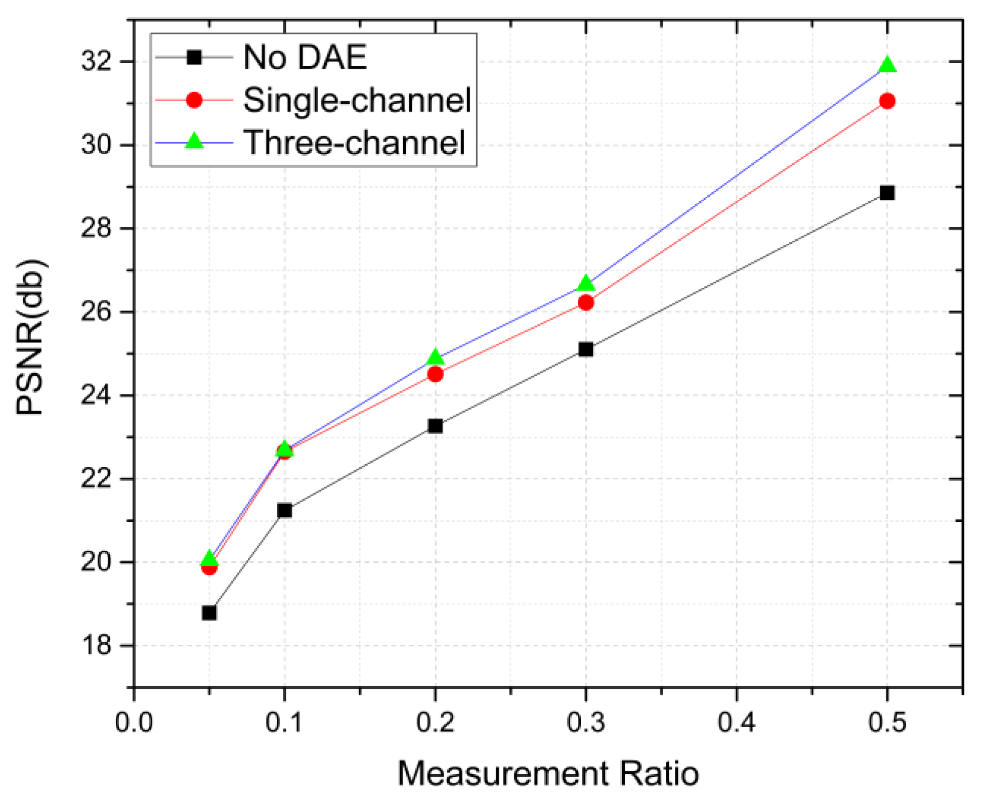
| Mean PSNR | No DAE | 18.786 | 21.240 | 23.265 | 25.106 | 28.859 |
| Single-channel | 19.886 | 22.650 | 24.510 | 26.228 | 31.058 | |
| Three-channel | 20.053 | 22.684 | 24.880 | 26.653 | 31.888 |
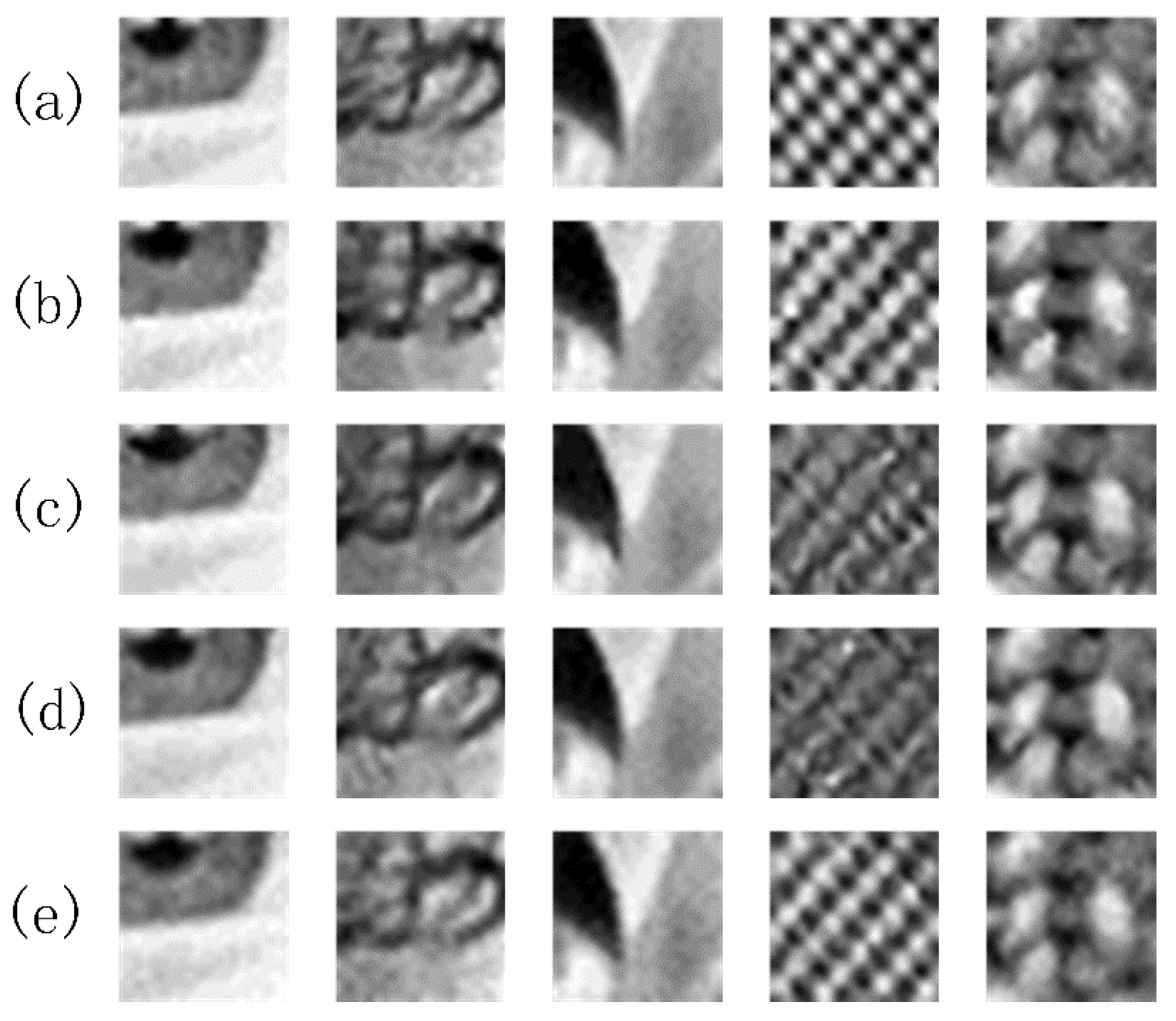
| Image Name | Methods | MR = 0.05 | MR = 0.1 | MR = 0.2 | MR = 0.3 | MR = 0.5 |
|---|---|---|---|---|---|---|
| eye | TVAL3 | 24.214 | 25.419 | 29.208 | 31.255 | 34.822 |
| ReconNet | 24.046 | 22.534 | 28.857 | 28.556 | 31.078 | |
| DR2Net | 21.999 | 27.876 | 29.522 | 30.799 | 30.404 | |
| DPAP | 25.183 | 27.789 | 29.748 | 31.682 | 34.793 | |
| hair | TVAL3 | 17.404 | 21.115 | 22.268 | 24.137 | 26.881 |
| ReconNet | 19.018 | 20.897 | 19.443 | 23.745 | 25.126 | |
| DR2Net | 18.533 | 21.479 | 22.367 | 18.735 | 24.301 | |
| DPAP | 19.043 | 21.305 | 22.555 | 23.049 | 25.651 | |
| parrot | TVAL3 | 23.284 | 23.030 | 27.597 | 29.275 | 34.395 |
| ReconNet | 22.736 | 26.245 | 27.647 | 16.051 | 18.995 | |
| DR2Net | 22.591 | 22.188 | 31.648 | 33.288 | 31.704 | |
| DPAP | 24.389 | 27.158 | 27.300 | 30.633 | 37.639 | |
| babara | TVAL3 | 12.585 | 16.159 | 18.865 | 21.274 | 26.366 |
| ReconNet | 12.737 | 16.261 | 16.501 | 18.955 | 24.574 | |
| DR2Net | 13.012 | 15.798 | 14.681 | 19.360 | 19.726 | |
| DPAP | 12.661 | 16.938 | 19.944 | 23.777 | 29.377 | |
| hat | TVAL3 | 17.512 | 18.754 | 21.815 | 22.878 | 26.960 |
| ReconNet | 19.362 | 21.045 | 22.839 | 24.133 | 25.811 | |
| DR2Net | 18.913 | 20.605 | 23.048 | 23.654 | 23.530 | |
| DPAP | 18.983 | 21.142 | 23.266 | 23.638 | 29.026 | |
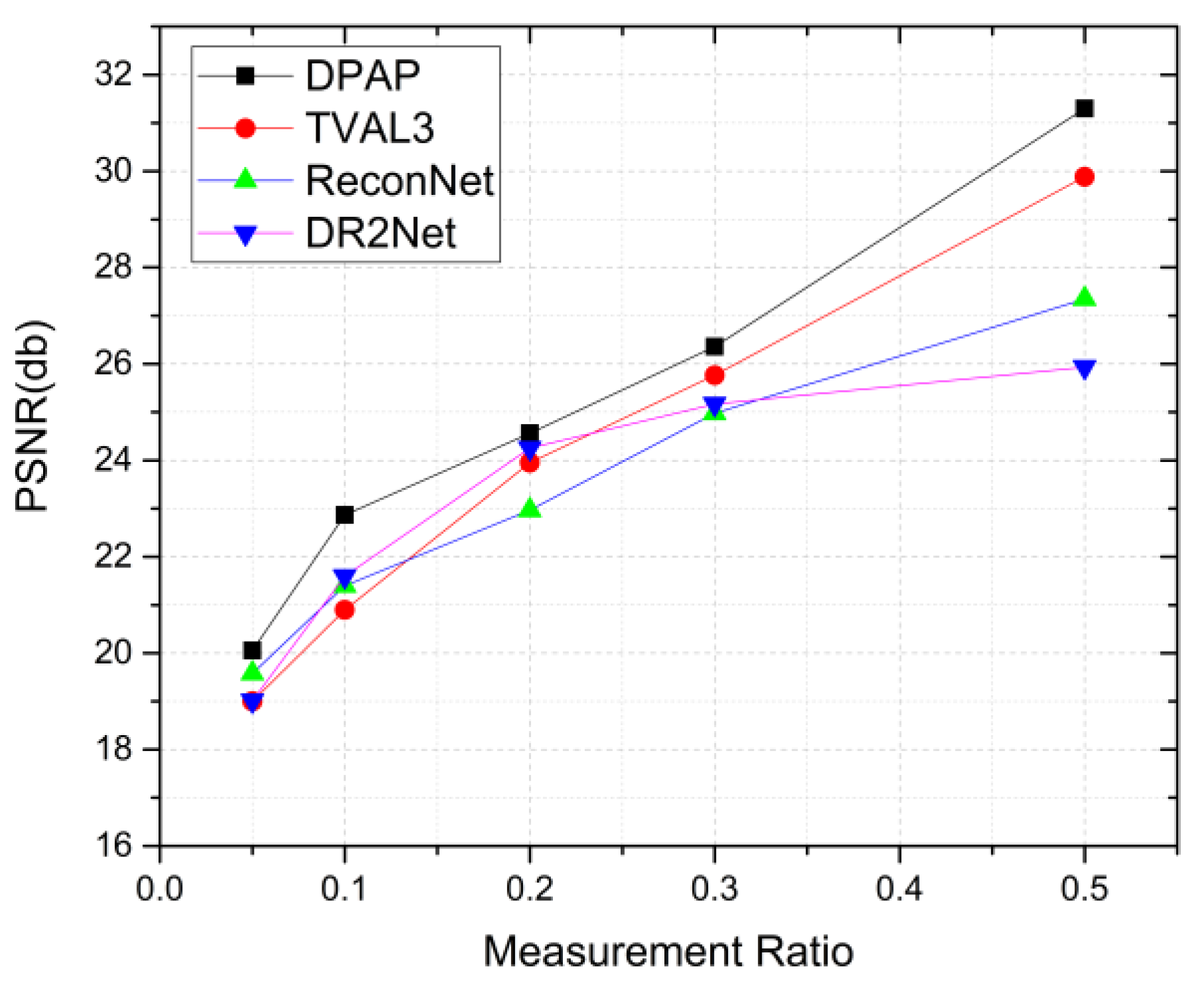
| Mean PSNR | TVAL3 | 19.000 | 20.895 | 23.951 | 25.764 | 29.885 |
| ReconNet | 19.580 | 21.397 | 22.967 | 24.977 | 27.346 | |
| DR2Net | 19.014 | 21.593 | 24.253 | 25.167 | 25.933 | |
| DPAP | 20.052 | 22.866 | 24.563 | 26.356 | 31.297 |
Publisher’s Note: MDPI stays neutral with regard to jurisdictional claims in published maps and institutional affiliations. |
© 2022 by the authors. Licensee MDPI, Basel, Switzerland. This article is an open access article distributed under the terms and conditions of the Creative Commons Attribution (CC BY) license (https://creativecommons.org/licenses/by/4.0/).
Share and Cite
Lin, J.; Yan, Q.; Lu, S.; Zheng, Y.; Sun, S.; Wei, Z. A Compressed Reconstruction Network Combining Deep Image Prior and Autoencoding Priors for Single-Pixel Imaging. Photonics 2022, 9, 343. https://doi.org/10.3390/photonics9050343
Lin J, Yan Q, Lu S, Zheng Y, Sun S, Wei Z. A Compressed Reconstruction Network Combining Deep Image Prior and Autoencoding Priors for Single-Pixel Imaging. Photonics. 2022; 9(5):343. https://doi.org/10.3390/photonics9050343
Chicago/Turabian StyleLin, Jian, Qiurong Yan, Shang Lu, Yongjian Zheng, Shida Sun, and Zhen Wei. 2022. "A Compressed Reconstruction Network Combining Deep Image Prior and Autoencoding Priors for Single-Pixel Imaging" Photonics 9, no. 5: 343. https://doi.org/10.3390/photonics9050343
APA StyleLin, J., Yan, Q., Lu, S., Zheng, Y., Sun, S., & Wei, Z. (2022). A Compressed Reconstruction Network Combining Deep Image Prior and Autoencoding Priors for Single-Pixel Imaging. Photonics, 9(5), 343. https://doi.org/10.3390/photonics9050343