Infrared Small Target Detection by Modified Density Peaks Searching and Local Gray Difference

Abstract
:1. Introduction
- A local heterogeneity indicator is proposed as a density feature to suppress high-brightness clutter;
- The efficiency of the algorithm is improved by iterative search;
- The LGD is proposed to describe the local contrast of candidate points, which highlights the targets better.
2. Density Peaks Searching
2.1. Density Peaks Searching
2.2. Shortcomings of DPS-GVR
3. Proposed Method
3.1. Modified Density Peaks Searching
3.1.1. Local Heterogeneity Indicator
3.1.2. Modified Density Peaks Searching Algorithm
- All of elements in D(k) are sorted from large to small, and the index of the sorted elements are represented as Ides;
- Traverse Ides, for each element (i, j) in Ides, execute 3, until all elements in the signed matrix S(k) are 1. Then stop the traversal and execute 4;
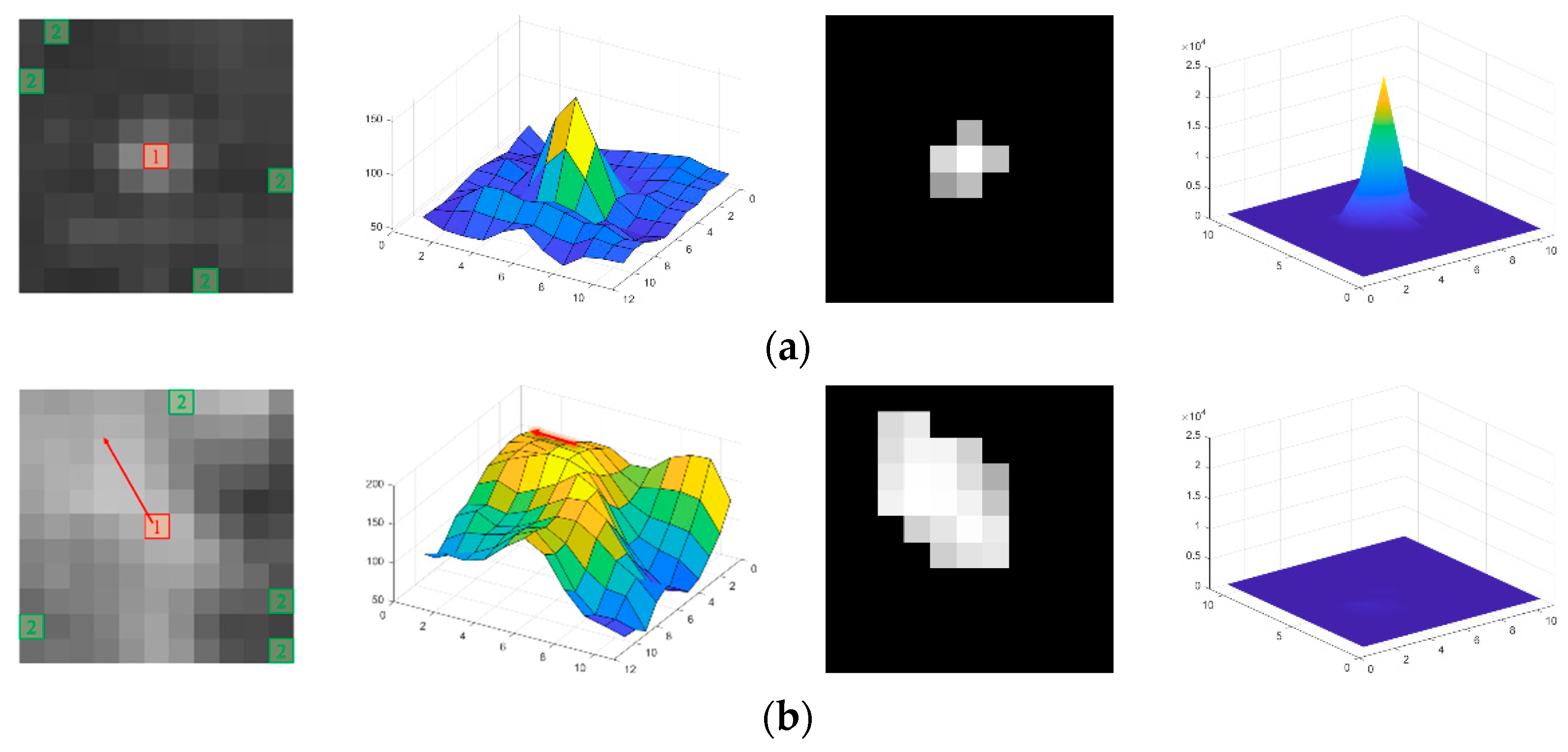
- Let S(k) (i, j) = 1. As shown in Figure 4b, U(i, j) represents an area of 3 × 3 window centered at (i, j) in D(k), for each point (s, t) in U(i, j), if S(k) (s, t) = 0: let S(k) (s, t) = 1, D(k) (s, t) = 0, the corresponding points of D(k) (s, t) and D(k) (i, j) in ρ are denoted as p and q, respectively. The δ-distance of point p can be calculated by Equation (7)
- Scale D(k) to half of the original, keep the points larger than 0 in D(k). Every element in the result D(k+1) can be calculated by Equation (8); the area represented by V(i, j) is shown in Figure 4b. Define the signed matrix S(k+1); every element in S(k+1) can be can be calculated by Equation (9). Then let k = k + 1.
| Algorithm 1 Modified Density Peaks Searching. |
| Input: Infrared image I ϵ ℝw×h |
| Output: Candidate target pixels set C |
| 1: Initialize: ρ = 0w×h, δ = 0w×h. |
| 2: Calculate the density ρ according to Equation (5). |
| 3: D(1) = ρ, S(1) = 0, k = 1, [m, n] = size(D(1)). |
| 4: while m > 1 or n > 1 |
| 5: Sort all elements in D(k) in descending order. The index vector of the sorted result is Ides. |
| 6: for each index (i, j) in Ides do |
| 7: S(k) (i, j) = 1. |
| 8: for (s, t) in U(i, j) do |
| 9: if S(k) (s, t) = 0 |
| 10: S(k) (s, t) =1, D(k) (s, t) = 0, calculate δ by Equation (7) |
| 11: end if |
| 12: end for |
| 13: end for |
| 14: Generate matrix D(k+1) = 0m/2×n/2, S(k+1) = 0m/2×n/2. |
| 15: The value of the pixel (i, j) in the D(k+1) is obtained by (8). |
| 16: The value of the pixel (i, j) in the S(k+1) is obtained by (9). |
| 17: [m, n] = size(D(k+1)), k = k + 1. |
| 18: end while |
| 19: For the last pixel i in D(k), δi = maxj(dij). |
| 20: Calculate the density peaks clustering index γ according to (6). |
| 21: Sort all the pixels by γ in descending order. |
| 22: Output candidate target pixels set C with the first np pixels. |
3.2. Local Gray Difference Indicator
3.3. Implementation of the Proposed Method
| Algorithm 2 The Proposed Detection Method Based on LGD. |
| Input: Infrared image I ϵ ℝw×h |
| Output: Detection result |
| 1: Obtain candidate target pixels set C according to Algorithm 1. |
| 2: for any ck ϵ C do |
| 3: Obtain core area Ak by RW algorithm. |
| 4: for any p ϵ Ak do |
| 5: Compute the MGDEp according to (12). |
| 6: end for |
| 7: Compute the according to (13). |
| 8: end for |
| 9: Extract targets from candidate target pixels using adaptive threshold in (14). |
4. Experimental Results and Analysis
4.1. Experimental Setup
4.1.1. Datasets and Baseline Methods
4.1.2. Evaluation Metrics
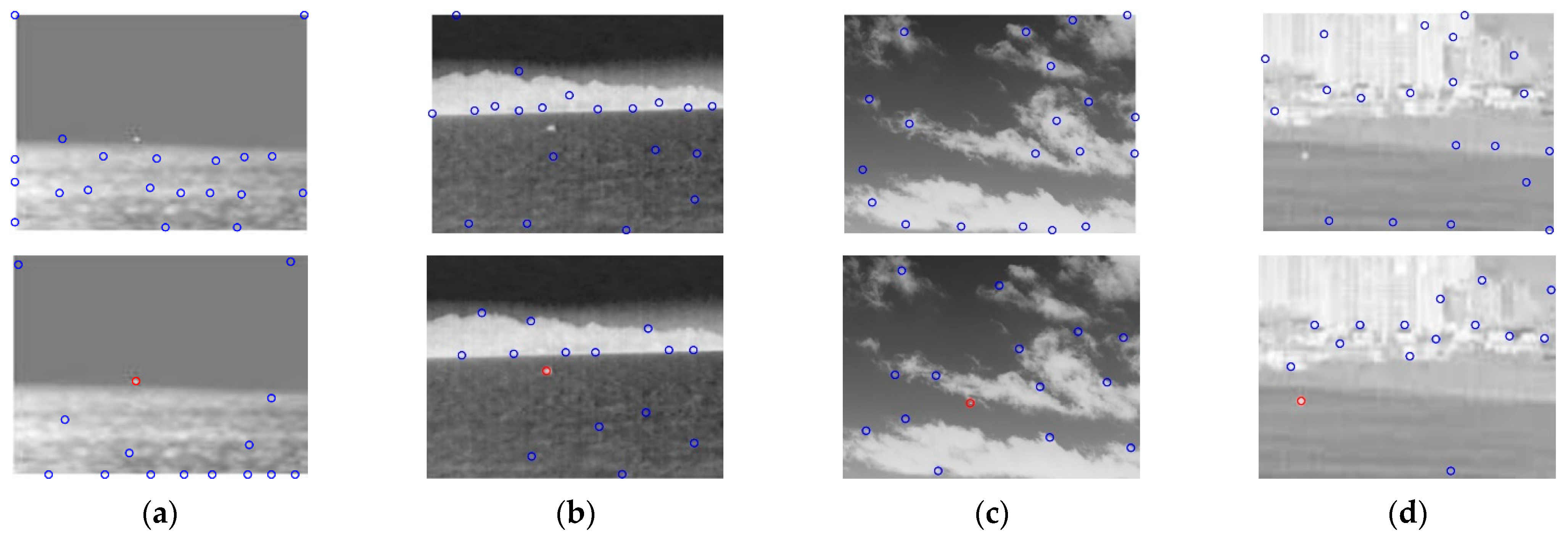
4.2. Anti-Noise Performance
4.3. Image Quality
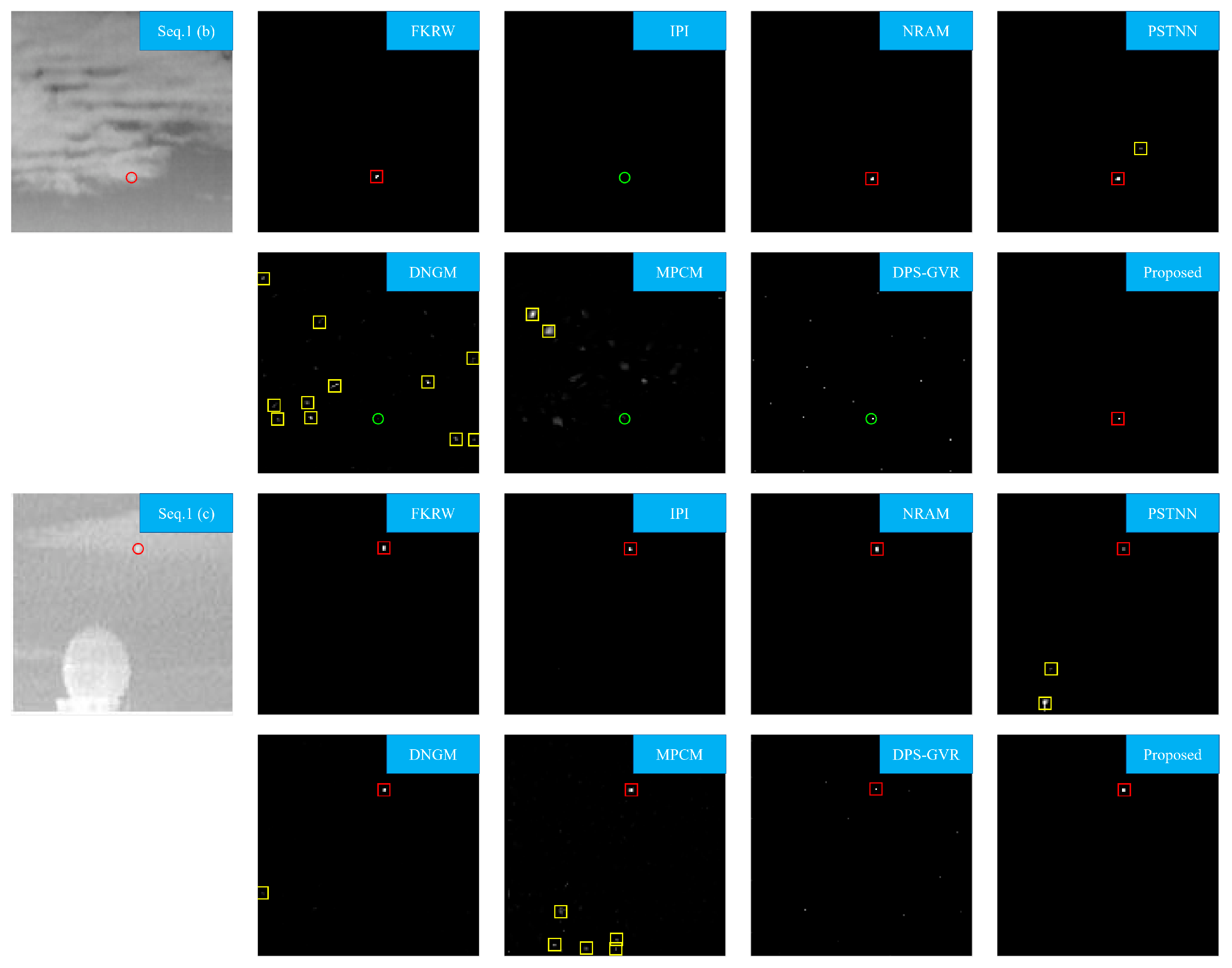
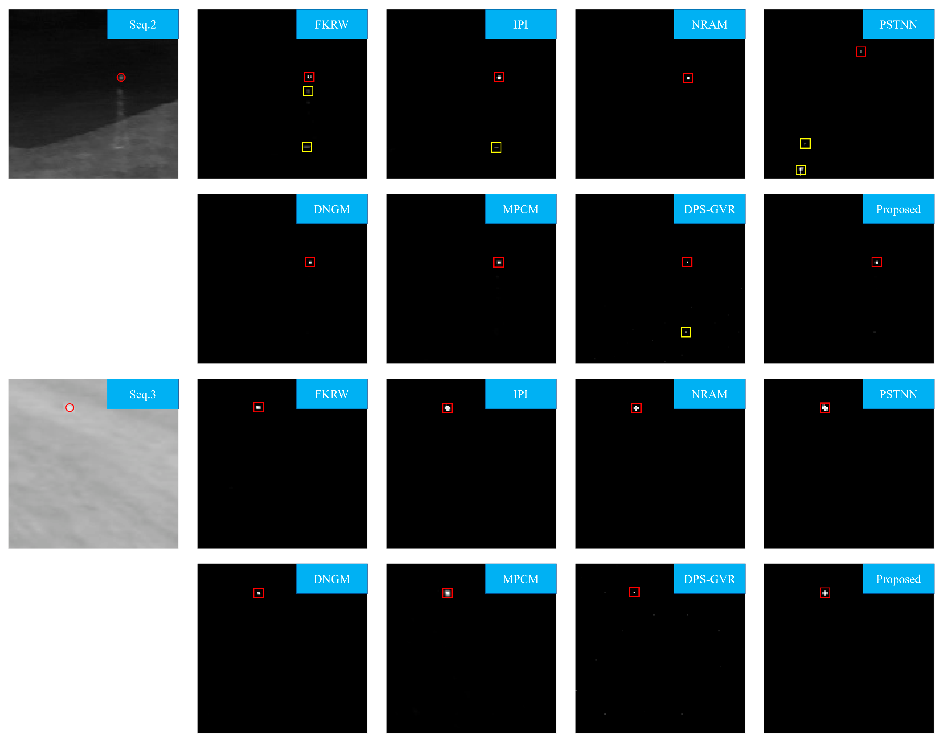
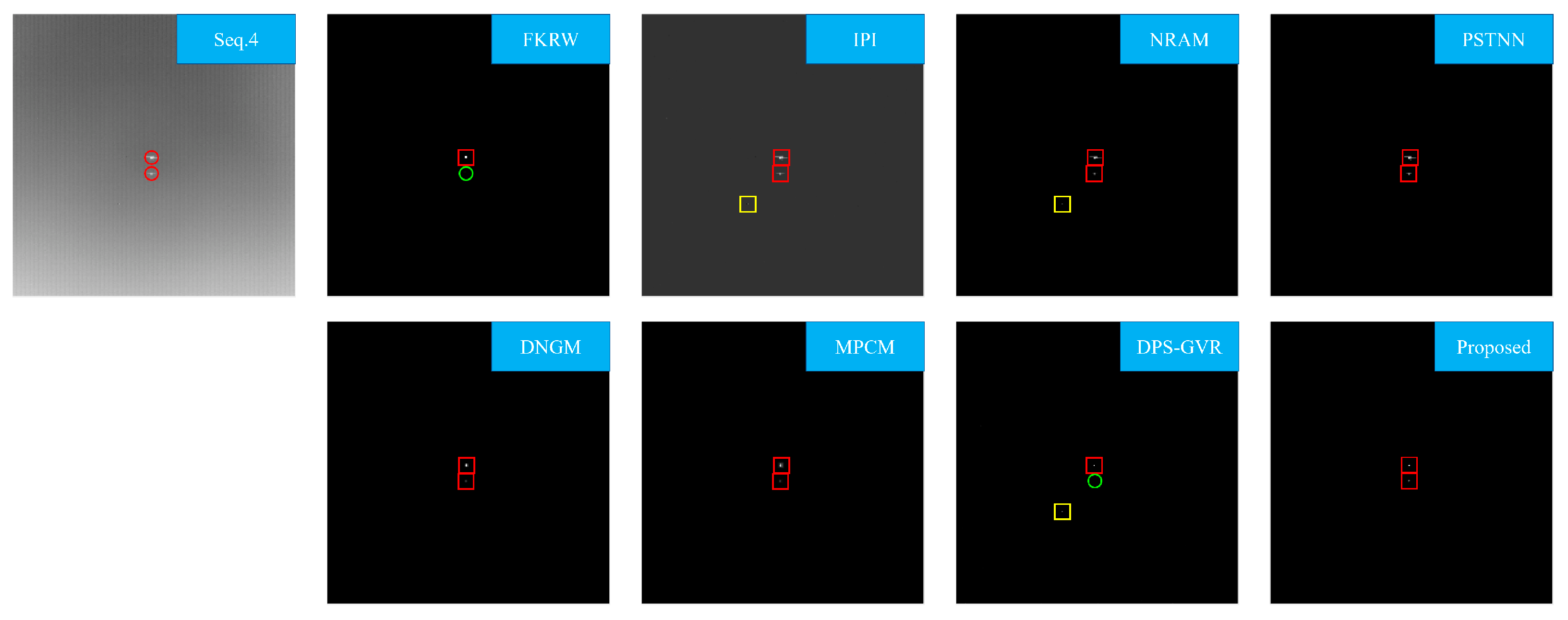
4.4. Detection Performance
4.5. Running Speed
5. Conclusions
Author Contributions
Funding
Data Availability Statement
Conflicts of Interest
References
- Chen, Y.; Song, B.; Wang, D.; Guo, L. An effective infrared small target detection method based on the human visual attention. Infrared Phys. Technol. 2018, 95, 128–135. [Google Scholar] [CrossRef]
- Kwan, C.; Larkin, J. Detection of Small Moving Objects in Long Range Infrared Videos from a Change Detection Perspective. Photonics 2021, 8, 394. [Google Scholar] [CrossRef]
- Li, W.; Zhao, M.; Deng, X.; Li, L.; Li, L.; Zhang, W. Infrared Small Target Detection Using Local and Nonlocal Spatial Information. IEEE J. Sel. Top. Appl. Earth Obs. Remote Sens. 2019, 12, 3677–3689. [Google Scholar] [CrossRef]
- Liu, R.; Wang, D.; Jia, P.; Sun, H. An Omnidirectional Morphological Method for Aerial Point Target Detection Based on Infrared Dual-Band Model. Remote Sens. 2018, 10, 1054. [Google Scholar] [CrossRef] [Green Version]
- Yang, P.; Dong, L.; Xu, W. Infrared Small Maritime Target Detection Based on Integrated Target Saliency Measure. IEEE J. Sel. Top. Appl. Earth Obs. Remote Sens. 2021, 14, 2369–2386. [Google Scholar] [CrossRef]
- Liu, D.; Cao, L.; Li, Z.; Liu, T.; Che, P. Infrared Small Target Detection Based on Flux Density and Direction Diversity in Gradient Vector Field. IEEE J. Sel. Top. Appl. Earth Obs. Remote Sens. 2018, 11, 2528–2554. [Google Scholar] [CrossRef]
- Zhao, M.; Li, L.; Li, W.; Tao, R.; Li, L.; Zhang, W. Infrared Small-Target Detection Based on Multiple Morphological Profiles. IEEE Trans. Geosci. Remote Sens. 2021, 59, 6077–6091. [Google Scholar] [CrossRef]
- Deng, H.; Sun, X.; Zhou, X. A Multiscale Fuzzy Metric for Detecting Small Infrared Targets Against Chaotic Cloudy/Sea-Sky Backgrounds. IEEE Trans. Cybern. 2019, 49, 1694–1707. [Google Scholar] [CrossRef]
- Cao, X.; Rong, C.; Bai, X. Infrared Small Target Detection Based on Derivative Dissimilarity Measure. IEEE J. Sel. Top. Appl. Earth Obs. Remote Sens. 2019, 12, 3101–3116. [Google Scholar] [CrossRef]
- Deng, H.; Wei, Y.; Tong, M. Small target detection based on weighted self-information map. Infrared Phys. Technol. 2013, 60, 197–206. [Google Scholar] [CrossRef]
- Zhao, M.; Li, W.; Li, L.; Hu, J.; Ma, P.; Tao, R. Single-Frame Infrared Small-Target Detection: A Survey. IEEE Geosci. Remote Sens. Mag. 2022, in press. [Google Scholar] [CrossRef]
- Bai, X.; Zhou, F. Analysis of new top-hat transformation and the application for infrared dim small target detection. Pattern Recognit. 2010, 43, 2145–2156. [Google Scholar] [CrossRef]
- Jianjun, Z.; Haoyin, L.; Fugen, Z. Infrared small target enhancement by using sequential top-hat filters. In Proceedings of the International Symposium on Optoelectronic Technology and Application 2014, Beijing, China, 13–15 May 2014. [Google Scholar]
- Suyog, D.D.; Meng Hwa, E.; Ronda, V.; Philip, C. Max-mean and max-median filters for detection of small targets. In Proceedings of the SPIE’s International Symposium on Optical Science, Engineering, and Instrumentation, Denver, CO, USA, 18 July 1999. [Google Scholar]
- Li, L.; Tang, Y.Y. Wavelet-hough transform with applications in edge and target detections. Int. J. Wavelets Multiresolution Inf. Processing 2006, 4, 567–587. [Google Scholar] [CrossRef]
- Soni, T.; Zeidler, J.R.; Ku, W.H. Performance evaluation of 2-D adaptive prediction filters for detection of small objects in image data. IEEE Trans. Image Processing 1993, 2, 327–340. [Google Scholar] [CrossRef]
- Bi, Y.; Chen, J.; Sun, H.; Bai, X. Fast Detection of Distant, Infrared Targets in a Single Image Using Multiorder Directional Derivatives. IEEE Trans. Aerosp. Electron. Syst. 2020, 56, 2422–2436. [Google Scholar] [CrossRef]
- Deng, H.; Sun, X.; Liu, M.; Ye, C.; Zhou, X. Small Infrared Target Detection Based on Weighted Local Difference Measure. IEEE Trans. Geosci. Remote Sens. 2016, 54, 4204–4214. [Google Scholar] [CrossRef]
- Gao, C.; Meng, D.; Yang, Y.; Wang, Y.; Zhou, X.; Hauptmann, A.G. Infrared Patch-Image Model for Small Target Detection in a Single Image. IEEE Trans. Image Processing 2013, 22, 4996–5009. [Google Scholar] [CrossRef]
- Zhang, L.; Peng, L.; Zhang, T.; Cao, S.; Peng, Z. Infrared Small Target Detection via Non-Convex Rank Approximation Minimization Joint l2,1 Norm. Remote Sens. 2018, 10, 1821. [Google Scholar] [CrossRef] [Green Version]
- Zhang, L.; Peng, Z. Infrared Small Target Detection Based on Partial Sum of the Tensor Nuclear Norm. Remote Sens. 2019, 11, 382. [Google Scholar] [CrossRef] [Green Version]
- Chen, C.L.P.; Li, H.; Wei, Y.; Xia, T.; Tang, Y.Y. A Local Contrast Method for Small Infrared Target Detection. IEEE Trans. Geosci. Remote Sens. 2014, 52, 574–581. [Google Scholar] [CrossRef]
- Han, J.; Ma, Y.; Zhou, B.; Fan, F.; Liang, K.; Fang, Y. A Robust Infrared Small Target Detection Algorithm Based on Human Visual System. IEEE Geosci. Remote Sens. Lett. 2014, 11, 2168–2172. [Google Scholar] [CrossRef]
- Wei, Y.; You, X.; Li, H. Multiscale patch-based contrast measure for small infrared target detection. Pattern Recognit. 2016, 58, 216–226. [Google Scholar] [CrossRef]
- Lv, P.; Sun, S.; Lin, C.; Liu, G. A method for weak target detection based on human visual contrast mechanism. IEEE Geosci. Remote Sens. Lett. 2018, 16, 261–265. [Google Scholar] [CrossRef]
- Wu, L.; Ma, Y.; Fan, F.; Wu, M.; Huang, J. A Double-Neighborhood Gradient Method for Infrared Small Target Detection. IEEE Geosci. Remote Sens. Lett. 2021, 18, 1476–1480. [Google Scholar] [CrossRef]
- Chen, Y.; Zhang, G.; Ma, Y.; Kang, J.U.; Kwan, C. Small Infrared Target Detection Based on Fast Adaptive Masking and Scaling With Iterative Segmentation. IEEE Geosci. Remote Sens. Lett. 2022, 19, 1–5. [Google Scholar] [CrossRef]
- Moradi, S.; Moallem, P.; Sabahi, M.F. Fast and robust small infrared target detection using absolute directional mean difference algorithm. Signal Processing 2020, 177, 107727. [Google Scholar] [CrossRef]
- Wang, C.; Wang, L. Multidirectional Ring Top-Hat Transformation for Infrared Small Target Detection. IEEE J. Sel. Top. Appl. Earth Obs. Remote Sens. 2021, 14, 8077–8088. [Google Scholar] [CrossRef]
- Deng, L.; Zhang, J.; Xu, G.; Zhu, H. Infrared small target detection via adaptive M-estimator ring top-hat transformation. Pattern Recognit. 2021, 112, 107729. [Google Scholar] [CrossRef]
- Deng, H.; Sun, X.; Liu, M.; Ye, C.; Zhou, X. Infrared small-target detection using multiscale gray difference weighted image entropy. IEEE Trans. Aerosp. Electron. Syst. 2016, 52, 60–72. [Google Scholar] [CrossRef]
- Xia, C.; Li, X.; Zhao, L. Infrared Small Target Detection via Modified Random Walks. Remote Sens. 2018, 10, 2004. [Google Scholar] [CrossRef] [Green Version]
- Grady, L. Random Walks for Image Segmentation. IEEE Trans. Pattern Anal. Mach. Intell. 2006, 28, 1768–1783. [Google Scholar] [CrossRef] [Green Version]
- Qin, Y.; Bruzzone, L.; Gao, C.; Li, B. Infrared Small Target Detection Based on Facet Kernel and Random Walker. IEEE Trans. Geosci. Remote Sens. 2019, 57, 7104–7118. [Google Scholar] [CrossRef]
- Qiu, Z.-B.; Ma, Y.; Fan, F.; Huang, J.; Wu, M.-H.; Mei, X.-G. A pixel-level local contrast measure for infrared small target detection. Def. Technol. 2021, in press. [Google Scholar] [CrossRef]
- Rodriguez, A.; Laio, A. Clustering by fast search and find of density peaks. Science 2014, 344, 1492–1496. [Google Scholar] [CrossRef] [Green Version]
- Huang, S.; Peng, Z.; Wang, Z.; Wang, X.; Li, M. Infrared Small Target Detection by Density Peaks Searching and Maximum-Gray Region Growing. IEEE Geosci. Remote Sens. Lett. 2019, 16, 1919–1923. [Google Scholar] [CrossRef]
- Zhu, Q.; Zhu, S.; Liu, G.; Peng, Z. Infrared Small Target Detection Using Local Feature-Based Density Peaks Searching. IEEE Geosci. Remote Sens. Lett. 2022, 19, 1–5. [Google Scholar] [CrossRef]
- Xia, C.; Li, X.; Zhao, L.; Yu, S. Modified Graph Laplacian Model With Local Contrast and Consistency Constraint for Small Target Detection. IEEE J. Sel. Top. Appl. Earth Obs. Remote Sens. 2020, 13, 5807–5822. [Google Scholar] [CrossRef]


| Frame Number | Frame Size | Targets | Target Size | Background | Clutter Description | |
|---|---|---|---|---|---|---|
| Seq.1 | 100 | 278 × 360, 128 × 128 | 141 | 3 × 3 to 9 × 9 | Building, sea, etc. | Heavy noise, salient strong edges |
| Seq.2 | 300 | 256 × 256 | 300 | 3 × 3 to 5 × 5 | Cloudy sky | Irregular cloud |
| Seq.3 | 180 | 256 × 256 | 300 | 6 × 6 to 11 × 11 | Sea | Sea-level background with much clutter |
| Seq.4 | 100 | 256 × 256 | 200 | 10 × 3, 3 × 2 | Sky | Banding noise, PNHB |
| Methods | Parameter Setting |
|---|---|
| MKRW | K = 4, p = 6, β = 200, window size: 11 × 11 |
| IPI | patch size: 50 × 50, sliding setp:10, , ε = 10−7 |
| NRAM | patch size: 50 × 50, sliding setp:10, , ε = 10−7, γ = −0.002 |
| PSTNN | patch size: 50 × 50, sliding setp:40, , ε = 10−7, γ = −0.002 |
| DNGM | N = 3 |
| MPCM | N = 3, 5, 7, 9, L = 3 |
| DSP-GVR | np = 20, nk = 0.0015 × mn |
| Proposed | l = 4, d = 11, m = 5, τ = 8 |
| Original Image | Enhanced Image | Nosie-Added Image | Enhanced Image | |
|---|---|---|---|---|
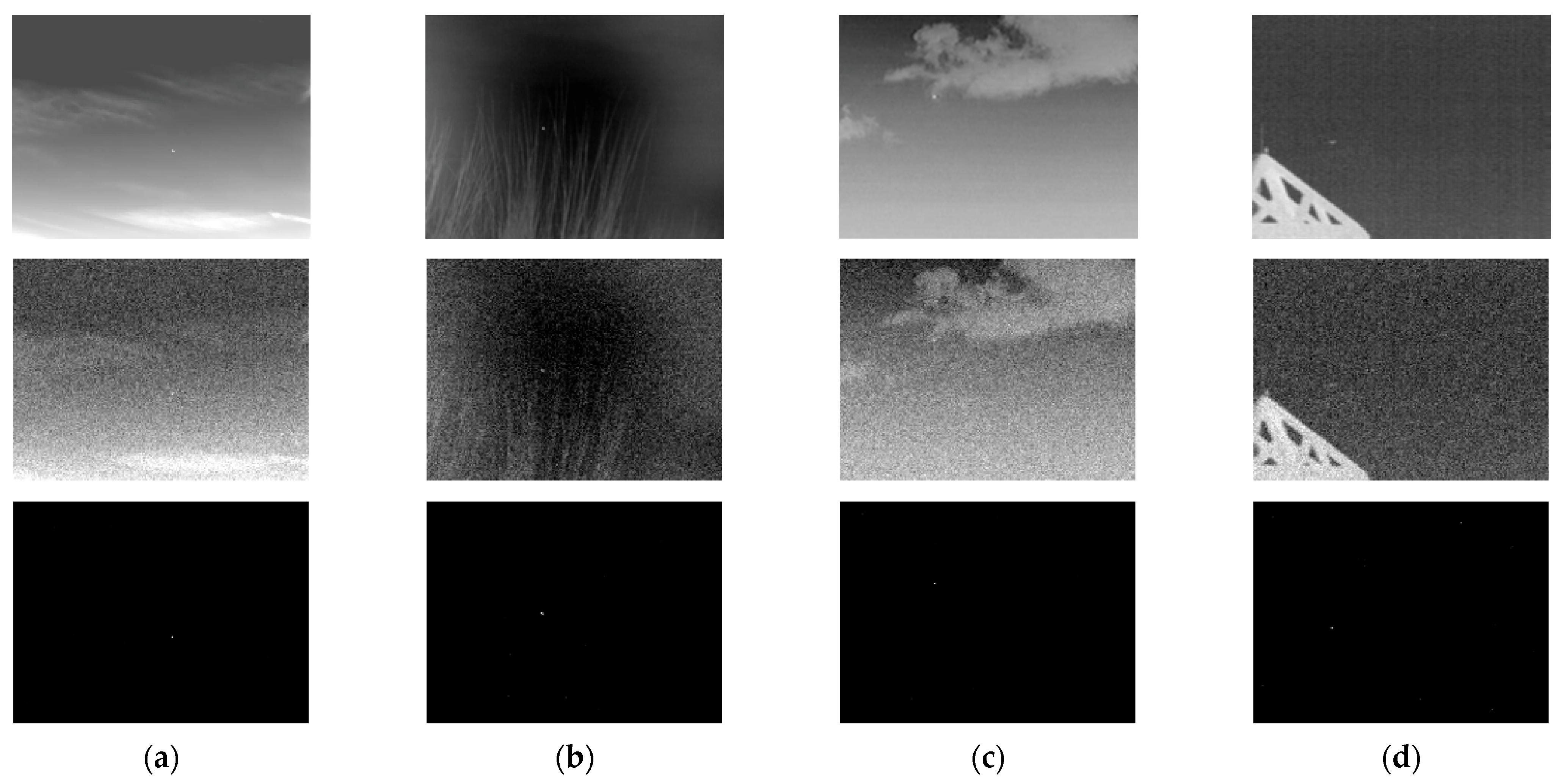
| Figure 7a | 2.8262 | 31.5807 | 1.7068 | 27.3232 |
| Figure 7b | 6.3872 | 23.0794 | 3.4259 | 22.9246 |
| Figure 7c | 5.8426 | 21.6889 | 2.8987 | 21.0840 |
| Figure 7d | 7.2077 | 26.3750 | 2.1380 | 24.2110 |
| FKRW | IPI | NRAM | PSTNN | DNGM | MPCM | DPS-GVR | Proposed | ||
|---|---|---|---|---|---|---|---|---|---|
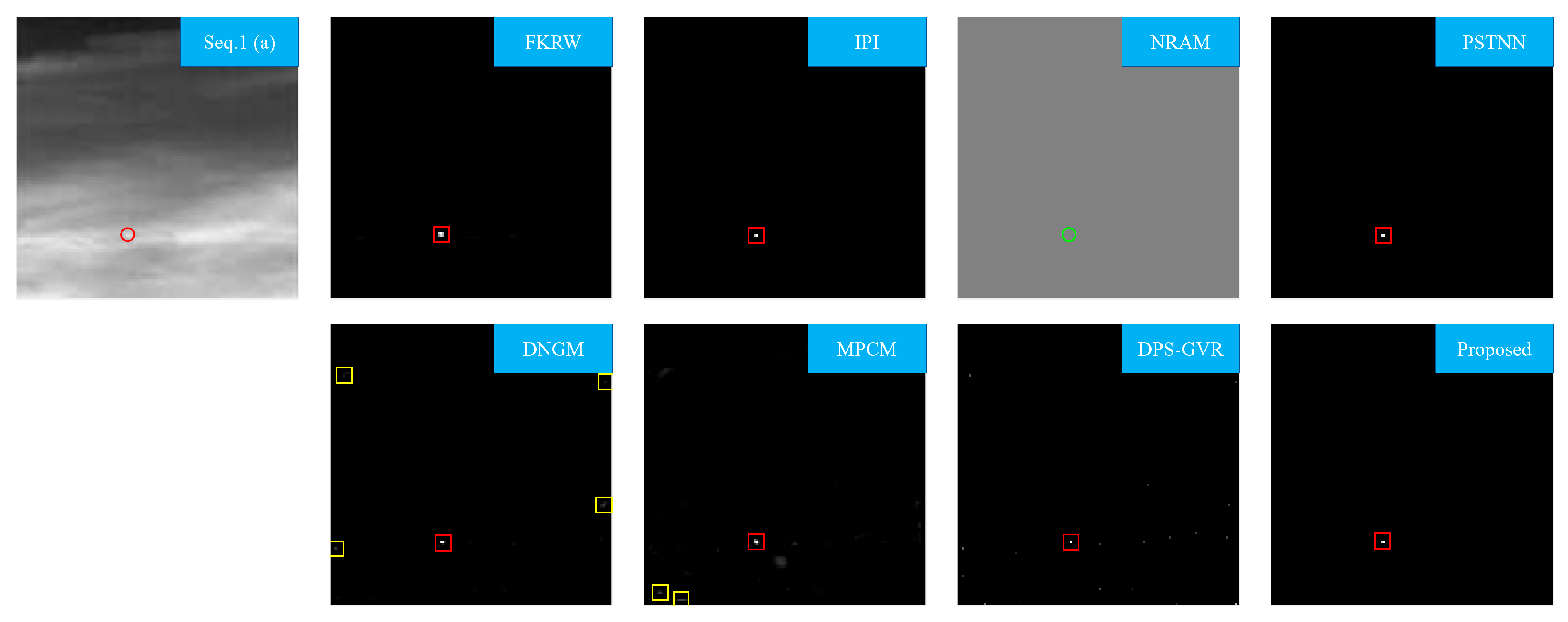
| Seq.1 | BSF | 311.51 | 32.41 | 94.36 | 28.94 | 175.11 | 23.95 | 42.04 | 329.79 |
| INF in BSF | 0 | 5 | 20 | 9 | 0 | 0 | 0 | 14 | |
| CG | 5.45 | 5.25 | 5.19 | 5.62 | 6.92 | 7.13 | 5.27 | 6.49 | |
| Seq.2 | BSF | 639.17 | 424.56 | 102.54 | 36.42 | 305.86 | 15.46 | 41.93 | 2.17 × 10³ |
| INF in BSF | 12 | 72 | 127 | 105 | 0 | 0 | 0 | 102 | |
| CG | 8.45 | 9.47 | 10.73 | 9.83 | 10.72 | 11.0361 | 11.23 | 11.71 | |
| Seq.3 | BSF | 164.93 | 561.83 | 40.72 | 28.38 | 320.08 | 40.71 | 14.24 | 421.03 |
| INF in BSF | 38 | 43 | 56 | 93 | 0 | 0 | 0 | 35 | |
| CG | 6.22 | 5.72 | 5.06 | 5.43 | 6.62 | 6.62 | 6.48 | 6.55 | |
| Seq.4 | BSF | 174.99 | 65.07 | 92.15 | 133.19 | 559.60 | 47.60 | 65.66 | 5.00 × 10³ |
| INF in BSF | 0 | 0 | 0 | 50 | 0 | 0 | 0 | 76 | |
| CG | 3.35 | 3.11 | 3.98 | 4.08 | 3.28 | 3.27 | 2.55 | 3.81 |
| FKRW | IPI | NRAM | PSTNN | DNGM | MPCM | DPS-GVR | Proposed | |
|---|---|---|---|---|---|---|---|---|
| Seq.1 | 0.1468 | 3.4239 | 1.0260 | 0.1715 | 2.1835 | 0.0331 | 0.3626 | 0.0840 |
| Seq.2 | 0.2330 | 3.4830 | 1.2912 | 0.2806 | 3.1556 | 0.0724 | 0.4964 | 0.1336 |
| Seq.3 | 0.2270 | 3.2550 | 1.2408 | 0.2696 | 3.0464 | 0.0732 | 0.5332 | 0.1376 |
| Seq.4 | 0.1080 | 3.6193 | 1.6296 | 0.1542 | 3.1383 | 0.0380 | 0.5648 | 0.1322 |
Publisher’s Note: MDPI stays neutral with regard to jurisdictional claims in published maps and institutional affiliations. |
© 2022 by the authors. Licensee MDPI, Basel, Switzerland. This article is an open access article distributed under the terms and conditions of the Creative Commons Attribution (CC BY) license (https://creativecommons.org/licenses/by/4.0/).
Share and Cite
Wu, M.; Chang, L.; Yang, X.; Jiang, L.; Zhou, M.; Gao, S.; Pan, Q. Infrared Small Target Detection by Modified Density Peaks Searching and Local Gray Difference. Photonics 2022, 9, 311. https://doi.org/10.3390/photonics9050311
Wu M, Chang L, Yang X, Jiang L, Zhou M, Gao S, Pan Q. Infrared Small Target Detection by Modified Density Peaks Searching and Local Gray Difference. Photonics. 2022; 9(5):311. https://doi.org/10.3390/photonics9050311
Chicago/Turabian StyleWu, Mo, Lin Chang, Xiubin Yang, Li Jiang, Meili Zhou, Suining Gao, and Qikun Pan. 2022. "Infrared Small Target Detection by Modified Density Peaks Searching and Local Gray Difference" Photonics 9, no. 5: 311. https://doi.org/10.3390/photonics9050311
APA StyleWu, M., Chang, L., Yang, X., Jiang, L., Zhou, M., Gao, S., & Pan, Q. (2022). Infrared Small Target Detection by Modified Density Peaks Searching and Local Gray Difference. Photonics, 9(5), 311. https://doi.org/10.3390/photonics9050311