Accelerated Phase Deviation Elimination for Measuring Moving Object Shape with Phase-Shifting-Profilometry

Abstract

Eliminating the phase deviation caused by object motion plays a vital role to obtain the precise phase map to recover the object shape with phase-shifting-profilometry. Pixel-by-pixel phase retrieval using the least-squares algorithm has been widely employed to eliminate the phase deviation caused by moving object. However, pixel-level operation can only eliminate phase deviation within a limited range, and will bring high computational burden. In this paper, we propose an image-level phase compensation method with stochastic gradient descent (SGD) algorithm to accelerate the phase deviation elimination. Since the iteration calculation is implemented at the image-level, the proposed method can accelerate the convergence significantly. Furthermore, since the proposed algorithm is able to correct the phase deviation within $(-\pi ,\pi )$, the algorithm can tolerate a greater motion range. In addition to simulation experiments, we consider 2-D motion of the object, and conduct a series of comparative experiments to validate the effectiveness of the proposed method in a larger motion range.

1. Introduction

Fringe projection profilometry modulates the surface depth information of object into the phase maps of fringe patterns, which has been extensively adopted in modern industries to measure the 3D shape of object due to its high accuracy and non-contact characteristics [1,2,3]. To obtain the precise wrapped phase maps, phase-shifting-profilometry (PSP) is one of the most commonly used methods in fringe projection profilometry. In PSP, the digital projector illuminates the stationary object by a series of fringe patterns with equally spaced phase. Through the modulated fringe patterns and triangle relationship, the accurate surface height of the object can be reconstructed. However, the rapid growth of industrial inspection requires to recover the 3D shape of moving object is required to be recovered [4,5,6], thus reconstructing the surface of moving object with PSP has become a practical issue that should be considered [7,8,9].

When PSP based method is applied to recover the surface of moving object, the phase deviation caused by object motion often results in severe artifacts [6,7]. In order to reduce the phase deviation caused by motion, there are two main approaches. One is to capture the fringe patterns with high-speed photography hardware. Zheng et al. [10] develop a method based on PSP with projector defocusing for high speed 3D shape measurement and analyze the phase deviation model. However, use of high speed equipment [10,11,12,13,14] implies a significant increase in the cost and the complexity of system [15]. Another approach is to reduce the phase deviation caused by motion through phase compensation.

Based on this consideration, Lu et al. [1] propose to use a set of marks on the object surface to describe the rotation matrix and translation vector of the phase deviation, an iterative least-squares algorithm is presented to perform pixel-level phase compensation. Lu et al. [16] also extend the method to the case of 3-D movement of the object. Feng et al. [6] propose a robust motion-compensated method for three-step PSP, which corrects the phase deviation with adjacent pixels. To estimate phase deviation caused by the object motion, Wang et al. [17] apply the Hilbert transform to phase-shifted fringe patterns to generate another set of fringe patterns. This method is less computationally expensive, but there is an underlying assumption that requires the object to move slower than the camera speed. Wang et al. [18] also propose a novel motion-induced method using additional samplings. Given that the method needs to capture two fringe patterns in one cycle, the accuracy of the external trigger will affect the quality of the reconstruction result. Duan et al. [19] propose a method for 2-D moving objects by introducing an adaptive reference phase map and motion tracking based on the composite image. However, the method encounters challenges when objects perform a wide range of motion. Li et al. [20] redefine the order of the projected stripe patterns and use the Hilbert transformation to compensate for the motion-induced errors and improve the utilization of the stripe. Since these phase compensation methods are developed on pixel-level, they still suffer from high computational amount [21]. In order to reduce the computational burden, Guo et al. [22] develop a Fourier-based method using dual-frequency composite phase-shifted grating patterns to achieve region-level phase compensation. However, due to the limitations of FTP, the method might not be available on case of dynamically deformable objects [8]. On the other hand, these algorithms are effective only when the phase deviation is within a limited range. When the phase deviation exceeds this range, these algorithms will not converge, which means the object with large motion range could not be reconstructed by these algorithms.

In addition to the aforementioned methods, Spoorthi et al. [23] propose a phase compensation method with deep learning to improve the accuracy of measurement, but it requires a large number of actual phase values obtained by iterative method for learning. Moreover, there are other methods [24,25,26] that use deep learning to correct phase deviation caused by motion. In specific application scenario, a large amount of actual phase data calculated through iterative method is difficult to acquire, it is impractical to use the deep learning to calibrate the phase deviation caused by motion in industrial measurement right now. Therefore, it is still necessary to develop the phase compensation method with high efficiency and accuracy under common resources.

To our knowledge, the existing pixel-level iterative methods have been suffered by two problems: limited motion range of object, and high computational burden. In this paper, we propose an image-level phase compensation method with SGD algorithm to accelerate phase deviation elimination. In this method, the difference among deformed fringe patterns is used to construct the iterative expression, which can reduce the computational burden of pixel-level based methods significantly. Furthermore, in the proposed SGD algorithm, each update of the iteration will randomly select a gradient direction, so the algorithm can escape from the saddle point to find the global optimum. Therefore, the large phase deviation can be eliminated effectively, which means our proposed method can reconstruct the object with larger motion range than existing methods.

2. Problem Formulation

PSP is one of the most promising approaches of 3-D shape reconstruction. Under the N-step PSP scenarios, $I_n(x,y)$ is the n-th deformed fringe patterns captured from the object, it can be described respectively as:

$$I_n(x,y)=a(x,y)+bcos(\omega y+\mathsf{\Phi }(x,y)+\frac{2\pi n}{N})$$

(1)

where $\left\{n\right|n\in \{0,1,\dots ,N-1\}\}$; $a(x,y)$ is the background ambient light intensity; b is the amplitude of the intensity of fringe patterns; $\omega$ is the angular frequency of fringe projection; $\omega y$ is the phase of the reference plane along the direction perpendicular to the fringe; $\mathsf{\Phi }(x,y)$ is the phase under the modulation of object height information; $\frac{2\pi n}{N}$ is the n-th preset phase shift of the fringe projection.

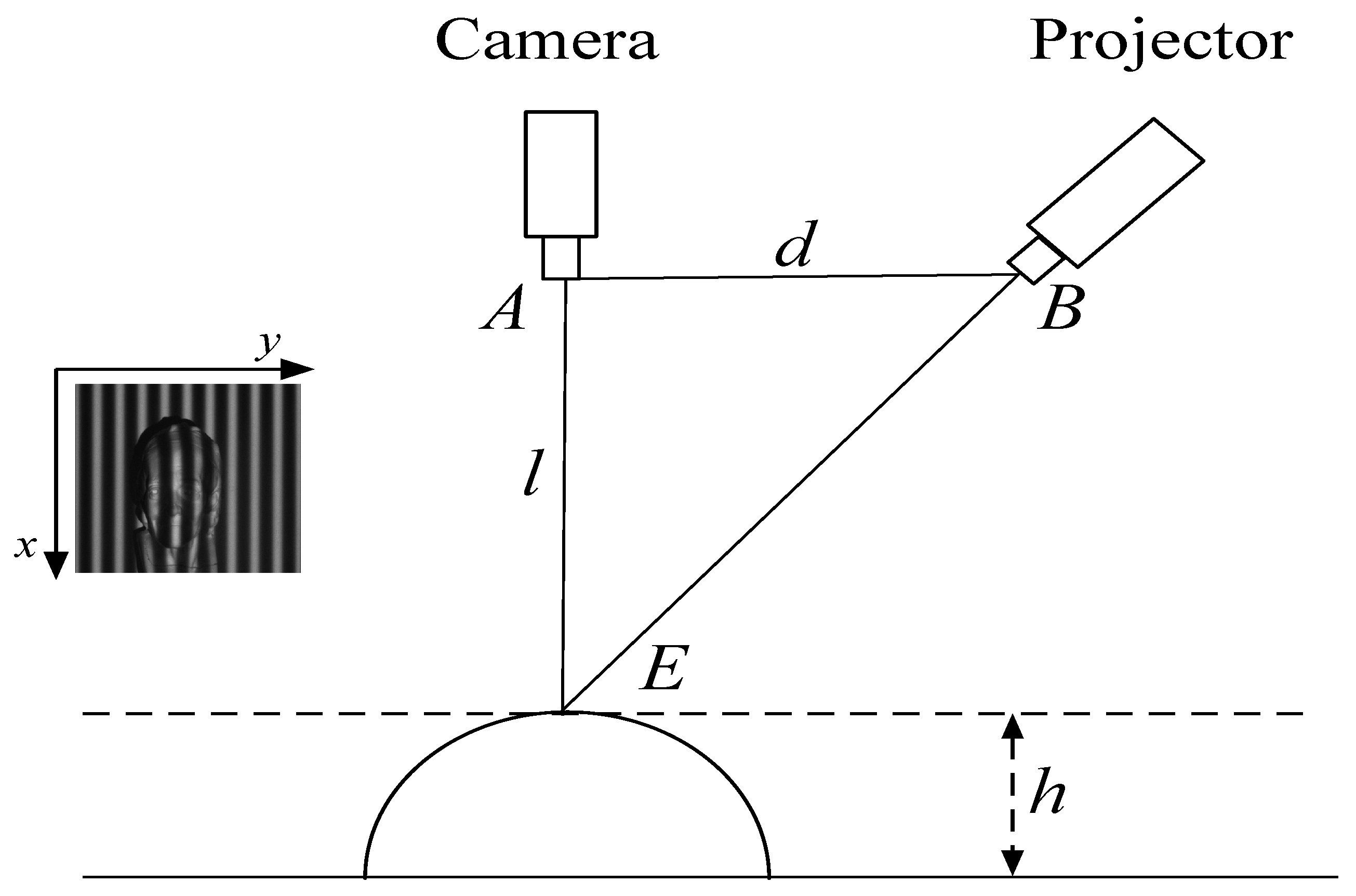
The direction of movement is shown in the Figure 1. A typical system consists of a camera A, and a projector B. The height h of a point E on the object surface is calculated by the modulated phase information. The distance between the camera and the projector is d, and the distance from the camera to the reference plane is $l+h$.

To simplify the analysis, we assume that the direction of the moving object is on the y-axis direction. When the direction of the y-axis is perpendicular to the direction of the fringe, we use $\mathrm{\Delta }{y}_n$ to describe displacement of the object in pixel on the n-th captured pattern. Through coordinates transformation, we yield the following:

$$\begin{array}{cc}\hfill I_n(x,y-\mathrm{\Delta }{y}_n)=& a(x,y)+bcos(\omega y+\mathsf{\Phi }(x,y)+(\frac{2\pi n}{N}-\omega \mathrm{\Delta }{y}_n))\hfill \end{array}$$

(2)

Since the pixels are discrete, the calculated result of $\mathrm{\Delta }{y}_n$ is an integer. We use $\mathrm{\Delta }{\mathsf{\Phi }}_n^{{}^{\prime }}=\frac{2\pi n}{N}-\omega \mathrm{\Delta }{y}_n=\frac{2\pi n}{N}-\omega \left[\mathrm{\Delta }{y}_n\right]$ to describe the actual phase to be calibrated. To further simplify the expression, we let ${\mathsf{\Phi }}^{{}^{\prime }}(x,y)$ as: ${\mathsf{\Phi }}^{{}^{\prime }}(x,y)=\omega y+\mathsf{\Phi }(x,y)$. The actual phase is difficult to solve directly and accurately due to the rounding error of $\mathrm{\Delta }{y}_n$.

In order to solve the actual phase, Lu et al. [1] propose a least-square iteration algorithm, which constructs the iteration equation with the gray value difference between the pixels with the same coordinate on different deformed fringe patterns. But this kind of algorithm always suffers from high computational complexity and falling to local optimal point due to its iterative operation at the pixel-level.

3. Derivation of the Proposed Algorithm

In order to accelerate the convergence, our proposed algorithm calculate the arithmetic average value of the difference between the different deformed fringe gray scales to construct the iteration equation, which reduces the computational complexity. The iteration equation illustrates the distance between the deformed fringe patterns difference and the actual phase. After obtaining an accurate deformed fringe patterns difference, we compensate the actual phase under this distance. If the accuracy of iteration calculation does not reach the stopping criterion, the actual phase to be calibrated is updated through the random gradient descent method, the iteration stops until the accuracy requirement is met.

3.1. Calculation of Deformed Fringe Patterns Difference

We use $K_{ij}$ to describe the absolute average value $〈\left|I_i(x,y)-I_j(x,y)\right|〉$ of the difference between the i-th deformed fringe patterns and the j-th deformed fringe patterns:

$$\begin{array}{cc}\hfill K_{ij}=& 〈\left|2bsin({\mathsf{\Phi }}^{{}^{\prime }}(x,y)+\frac{\mathrm{\Delta }{\mathsf{\Phi }}_i^{{}^{\prime }}+\mathrm{\Delta }{\mathsf{\Phi }}_j^{{}^{\prime }}}{2})\right|〉·|sin(\frac{\mathrm{\Delta }{\mathsf{\Phi }}_i^{{}^{\prime }}-\mathrm{\Delta }{\mathsf{\Phi }}_j^{{}^{\prime }}}{2})|\hfill \end{array}$$

(3)

where $\{i,j|i,j\in \{0,1,\dots ,N-1\},i\ne j\}$. Under grid motion, $〈\left|2bsin({\mathsf{\Phi }}^{{}^{\prime }}(x,y)+\frac{\mathrm{\Delta }{\mathsf{\Phi }}_i^{{}^{\prime }}+\mathrm{\Delta }{\mathsf{\Phi }}_j^{{}^{\prime }}}{2})\right|〉$ will be a fixed quantify. $c=〈\left|2bsin({\mathsf{\Phi }}^{{}^{\prime }}(x,y)+\frac{\mathrm{\Delta }{\mathsf{\Phi }}_i^{{}^{\prime }}+\mathrm{\Delta }{\mathsf{\Phi }}_j^{{}^{\prime }}}{2})\right|〉$ is the difference between the deformed fringe patterns to be calculated, which reflects the macroscopic differences between the patterns. We can calculate c through least square method [27] in Equation (4).

$$\left\{\begin{array}{c}\mathrm{\Delta }K=\sum _{i=1}^{N-1}\sum _{j=0}^{i-1}{\left(K_{ij}^{\prime }-K_{ij}\right)}^2\hfill \\ \frac{\partial \mathrm{\Delta }K}{\partial c}=\frac{\partial \mathrm{\Delta }K}{\partial \mathrm{\Delta }{\mathsf{\Phi }}_n^{{}^{\prime }}}=0\hfill \end{array}\right.$$

(4)

where $K_{ij}^{\prime }$ is the actual value of difference between deformed fringe patterns, and $K_{ij}$ is the value of difference between deformed fringe patterns, the actual value is the closest to the theoretical value. When $\frac{\partial \mathrm{\Delta }K}{\partial c}=\frac{\partial \mathrm{\Delta }K}{\partial \mathrm{\Delta }{\mathsf{\Phi }}_n^{{}^{\prime }}}=0$ is satisfied, $\mathrm{\Delta }K$ get the minimum value, c can be calculated iteratively as follows:

$$\begin{array}{cc}\hfill c=& \frac{{\sum }_{i=1}^{N-1}{\sum }_{j=0}^{i-1}{K}_{ij}^{\prime }|sin(\frac{\mathrm{\Delta }{\mathsf{\Phi }}_i^{{}^{\prime }}-\mathrm{\Delta }{\mathsf{\Phi }}_j^{{}^{\prime }}}{2})|}{{\sum }_{i=1}^{N-1}{\sum }_{j=0}^{i-1}{sin}^2(\frac{\mathrm{\Delta }{\mathsf{\Phi }}_i^{{}^{\prime }}-\mathrm{\Delta }{\mathsf{\Phi }}_j^{{}^{\prime }}}{2})}\hfill \\ \hfill =& \frac{4{\sum }_{i=1}^{N-1}{\sum }_{j=0}^{i-1}{K}_{ij}^{\prime }|sin(\frac{\mathrm{\Delta }{\mathsf{\Phi }}_i^{{}^{\prime }}-\mathrm{\Delta }{\mathsf{\Phi }}_j^{{}^{\prime }}}{2})|}{N(N-1)-2{\sum }_{i=1}^{N-1}{\sum }_{j=0}^{i-1}cos(\mathrm{\Delta }{\mathsf{\Phi }}_i^{{}^{\prime }}-\mathrm{\Delta }{\mathsf{\Phi }}_j^{{}^{\prime }})}\hfill \end{array}$$

(5)

With iterations, c will approach to the true value.

3.2. Differential Constrained Phase Compensation

After obtaining accurate c, we can calculate the actual phase $\mathrm{\Delta }{\mathsf{\Phi }}_n^{{}^{\prime }}$ under the constraints of c. We can take $\left\{m\right|m\in \{0,1,\dots ,N-1\}\}$, then the partial derivative $\frac{\partial \mathrm{\Delta }K}{\partial \mathrm{\Delta }{\mathsf{\Phi }}_n^{{}^{\prime }}}=0$ can be converted to the following:

$$\begin{array}{cc}\hfill & \frac{\partial }{\partial \mathrm{\Delta }{\mathsf{\Phi }}_m^{{}^{\prime }}}[\sum _{j=0}^{m-1}{\left(K_{mj}^{\prime }-c|sin(\frac{\mathrm{\Delta }{\mathsf{\Phi }}_m^{{}^{\prime }}-\mathrm{\Delta }{\mathsf{\Phi }}_j^{{}^{\prime }}}{2})|\right)}^2\hfill \\ \hfill & +\sum _{i=m+1}^{N-1}{\left(K_{im}^{\prime }-c|sin(\frac{\mathrm{\Delta }{\mathsf{\Phi }}_i^{{}^{\prime }}-\mathrm{\Delta }{\mathsf{\Phi }}_m^{{}^{\prime }}}{2})|\right)}^2]=0\hfill \end{array}$$

(6)

where $\{i|i\in \{m+1,m+2,...,N-1\}\}$ and $\{j|j\in \{0,1,...,m-1\}\}$. Through simplification, the solutions can be expressed as Equation (7).

$$\left\{\begin{array}{c}\hfill K_{mj}^{\prime }-c|sin(\frac{\mathrm{\Delta }{\mathsf{\Phi }}_m^{{}^{\prime }}-\mathrm{\Delta }{\mathsf{\Phi }}_j^{{}^{\prime }}}{2})|=0\\ \hfill K_{im}^{\prime }-c|sin(\frac{\mathrm{\Delta }{\mathsf{\Phi }}_i^{{}^{\prime }}-\mathrm{\Delta }{\mathsf{\Phi }}_m^{{}^{\prime }}}{2})|=0\end{array}\right.$$

(7)

When $c\ne 0$, $cos(\frac{\mathrm{\Delta }{\mathsf{\Phi }}_i-\mathrm{\Delta }{\mathsf{\Phi }}_m}{2})\ne 0$, Equation (7) can be expressed as:

$$\left\{\begin{array}{cc}\hfill \mathrm{\Delta }{\mathsf{\Phi }}_m^{{}^{\prime }}=\mathrm{\Delta }{\mathsf{\Phi }}_j^{{}^{\prime }}-2arcsin(\frac{K_{mj}^{\prime }}{c})& ,\mathrm{\Delta }{\mathsf{\Phi }}_m^{{}^{\prime }}<\mathrm{\Delta }{\mathsf{\Phi }}_j^{{}^{\prime }}\hfill \\ \hfill \mathrm{\Delta }{\mathsf{\Phi }}_m^{{}^{\prime }}=\mathrm{\Delta }{\mathsf{\Phi }}_j^{{}^{\prime }}+2arcsin(\frac{K_{mj}^{\prime }}{c})& ,\mathrm{\Delta }{\mathsf{\Phi }}_m^{{}^{\prime }}\ge \mathrm{\Delta }{\mathsf{\Phi }}_j^{{}^{\prime }}\hfill \\ \hfill \mathrm{\Delta }{\mathsf{\Phi }}_m^{{}^{\prime }}=\mathrm{\Delta }{\mathsf{\Phi }}_i^{{}^{\prime }}-2arcsin(\frac{K_{im}^{\prime }}{c})& ,\mathrm{\Delta }{\mathsf{\Phi }}_m^{{}^{\prime }}<\mathrm{\Delta }{\mathsf{\Phi }}_i^{{}^{\prime }}\hfill \\ \hfill \mathrm{\Delta }{\mathsf{\Phi }}_m^{{}^{\prime }}=\mathrm{\Delta }{\mathsf{\Phi }}_i^{{}^{\prime }}+2arcsin(\frac{K_{im}^{\prime }}{c})& ,\mathrm{\Delta }{\mathsf{\Phi }}_m^{{}^{\prime }}\ge \mathrm{\Delta }{\mathsf{\Phi }}_i^{{}^{\prime }}\hfill \end{array}\right.$$

(8)

We can calculate the arithmetic average of the actual phase to be calibrated as follows:

$$\begin{array}{cc}\hfill \overline{\mathrm{\Delta }{\mathsf{\Phi }}_m^{{}^{\prime }}}=& \frac{1}{N-1}[\sum _{i=0,i\ne m}^{N-1}\mathrm{\Delta }{\mathsf{\Phi }}_i^{{}^{\prime }}-2\sum _{i\in G_0}arcsin(\frac{K_{mi}^{\prime }}{c})\hfill \\ \hfill & +2\sum _{i\in G_1}arcsin(\frac{K_{mi}^{\prime }}{c})-2\sum _{i\in G_2}arcsin(\frac{K_{im}^{\prime }}{c})\hfill \\ \hfill & +2\sum _{i\in G_3}arcsin(\frac{K_{im}^{\prime }}{c})]\hfill \end{array}$$

(9)

where $G_0=\{x|x\in \{0,1,...,m-1\},\mathrm{\Delta }{\mathsf{\Phi }}_m^{{}^{\prime }}<\mathrm{\Delta }{\mathsf{\Phi }}_x^{{}^{\prime }}\}$, $G_1=\{x|x\in \{0,1,...,m-1\},\mathrm{\Delta }{\mathsf{\Phi }}_m^{{}^{\prime }}\ge \mathrm{\Delta }{\mathsf{\Phi }}_x^{{}^{\prime }}\}$, $G_2=\{x|x\in \{m+1,m+2,...,N-1\},\mathrm{\Delta }{\mathsf{\Phi }}_m^{{}^{\prime }}<\mathrm{\Delta }{\mathsf{\Phi }}_x^{{}^{\prime }}\}$, $G_3=\{x|x\in \{m+1,m+2,...,N-1\},\mathrm{\Delta }{\mathsf{\Phi }}_m^{{}^{\prime }}\ge \mathrm{\Delta }{\mathsf{\Phi }}_x^{{}^{\prime }}\}$.

3.3. Iteration Process

For the initial iteration, the actual phase to be calibrated is $\mathrm{\Delta }{\mathsf{\Phi }}_n^{{}^{\prime }}=\frac{2\pi n}{N}-\omega \left[\mathrm{\Delta }{y}_n\right]$. In subsequent iteration, the actual phase to be calibrated is the results obtained in the previous iteration. In each iteration, we make a judgment whether the result of this iteration meets the phase compensation accuracy requirement $ϵ$ as:

$$\sqrt{\frac{{\sum }_{i=0}^{N-1}{\left(\mathrm{\Delta }{\mathsf{\Phi }}_i^{{}^{\prime }(t)}-\mathrm{\Delta }{\mathsf{\Phi }}_i^{{}^{\prime }(t-1)}\right)}^2}{N}}<ϵ$$

(10)

where t is the number of iterations; $ϵ$ is the preset accuracy requirement to stop iterations. If the difference between two consecutive iterations satisfies Equation (10), we stop the iteration. Otherwise, the SGD method is introduced to obtain the new actual phase to be calibrated and proceed to the next iteration.

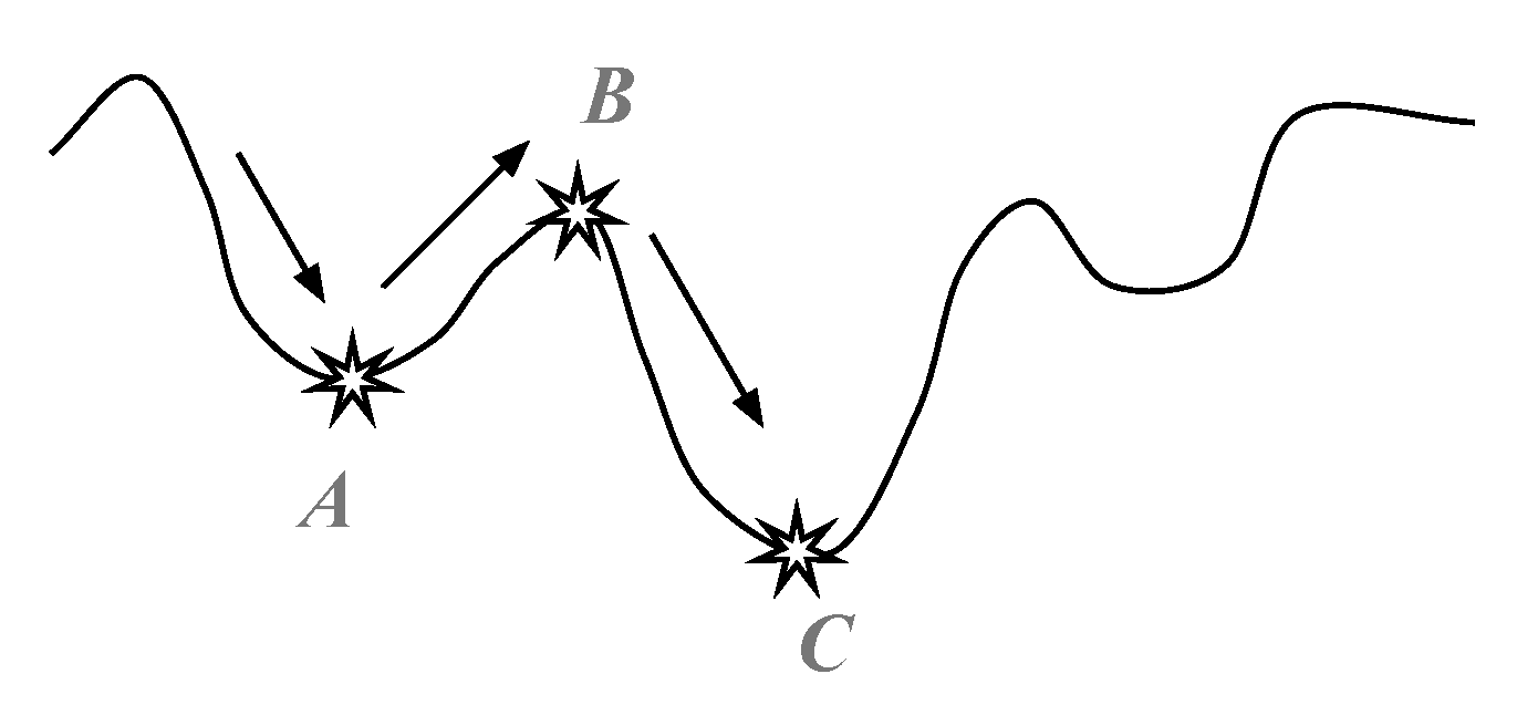
The reason for introducing SGD [28] is that the ordinary iteration process has no exploration mechanism, and it is easy to fall into the local optimum, as shown in Figure 2.

Before starting the SGD, we have precalculated the following parameters: the initial value of the descending step length s; the direction parameter r; the Euclidean distance of the actual phase compensation results of two consecutive iterations $dis(\mathrm{\Delta }{\mathsf{\Phi }}^{{}^{\prime }(t)},\mathrm{\Delta }{\mathsf{\Phi }}^{{}^{\prime }(t-1)})$; and the gradient value between the actual phase compensation results of consecutive iterations $g(\mathrm{\Delta }{\mathsf{\Phi }}^{{}^{\prime }(t)},\mathrm{\Delta }{\mathsf{\Phi }}^{{}^{\prime }(t-1)})$. Finally, we can calculate the input phase of the next generation $\mathrm{\Delta }{\mathsf{\Phi }}_n^{{}^{\prime }(t+1)}$.

We use Equation (11) to describe the updated descending step $s^{{}^{\prime }}$:

$$\begin{array}{cc}\hfill s^{{}^{\prime }}& =\frac{g(\mathrm{\Delta }{\mathsf{\Phi }}^{{}^{\prime }(t)},\mathrm{\Delta }{\mathsf{\Phi }}^{{}^{\prime }(t-1)})}{dis(\mathrm{\Delta }{\mathsf{\Phi }}^{{}^{\prime }(t)},\mathrm{\Delta }{\mathsf{\Phi }}^{{}^{\prime }(t-1)})}s=\frac{\mathrm{\Delta }{\mathsf{\Phi }}^{{}^{\prime }(t)},\mathrm{\Delta }{\mathsf{\Phi }}^{{}^{\prime }(t-1)}}{(t-(t-1))dis(\mathrm{\Delta }{\mathsf{\Phi }}^{{}^{\prime }(t)},\mathrm{\Delta }{\mathsf{\Phi }}^{{}^{\prime }(t-1)})}s\hfill \\ \hfill & =\frac{{\left(\begin{array}{c}\mathrm{\Delta }{\varphi }_0^{{}^{\prime }(t)}-\mathrm{\Delta }{\varphi }_0^{{}^{\prime }(t-1)},\mathrm{\Delta }{\varphi }_1^{{}^{\prime }(t)}-\mathrm{\Delta }{\varphi }_1^{{}^{\prime }(t-1)},\cdots ,\mathrm{\Delta }{\varphi }_{N-1}^{{}^{\prime }(t)}-\mathrm{\Delta }{\varphi }_{N-1}^{{}^{\prime }(t-1)}\end{array}\right)}^T}{dis(\mathrm{\Delta }{\mathsf{\Phi }}^{{}^{\prime }(t)},\mathrm{\Delta }{\mathsf{\Phi }}^{{}^{\prime }(t-1)})}s\hfill \end{array}$$

(11)

Similarly, specific to the n-th step size $s_n^{{}^{\prime }}$:

$$s_n^{{}^{\prime }}=\frac{\mathrm{\Delta }{\mathsf{\Phi }}_n^{{}^{\prime }(t)}-\mathrm{\Delta }{\mathsf{\Phi }}_n^{{}^{\prime }(t-1)}}{dis(\mathrm{\Delta }{\mathsf{\Phi }}^{{}^{\prime }(t)},\mathrm{\Delta }{\mathsf{\Phi }}^{{}^{\prime }(t-1)})}s$$

(12)

Then, we use Equation (13) and a random function $rand()$ to determine the gradient descent direction $dir(\mathrm{\Delta }{\mathsf{\Phi }}_n^{{}^{\prime }(t)})$:

$$dir(\mathrm{\Delta }{\mathsf{\Phi }}_n^{{}^{\prime }(t)})=\left\{\begin{array}{cc}\hfill 1& ,rand()\le p_0\hfill \\ \hfill -1& ,rand()>p_0\hfill \end{array}\right.$$

(13)

where $p_0=\frac{r}{1+r}$ reflects the probability along the fastest direction of the gradient. When $dir(\mathrm{\Delta }{\mathsf{\Phi }}_n^{{}^{\prime }(t)})=-1$, the iteration direction is changed to the opposite direction, otherwise no change will be made. Then, we can calculate $\mathrm{\Delta }{\mathsf{\Phi }}_n^{{}^{\prime }(t+1)}$ as follows:

$$\mathrm{\Delta }{\mathsf{\Phi }}_n^{{}^{\prime }(t+1)}=\mathrm{\Delta }{\mathsf{\Phi }}_n^{{}^{\prime }(t)}+dir(\mathrm{\Delta }{\mathsf{\Phi }}_n^{{}^{\prime }(t)})s_n^{{}^{\prime }}$$

(14)

The above derivation can also be extended to the object with 2D movement on the x-axis direction. The point on the object surface only has translational motion as the height is not changed with the movement. In the Figure 1, the phase deviation caused by the object moving in different directions can be solved using the proposed algorithm.

Summarily, the improvement of the calculation time of the proposed method in this paper can be explained by the calculation complexity. Obviously, the time complexity of our method is $O(M{N}^2)$, the time complexity of the pixel-level approaches represented by Ref. [16] is $O(M^{2}N)$, where the resolution of deformed fringe pattern is M, the number of deformed fringe patterns is N.

4. Experiments

In this section, we compare the performance between our method and other methods through experiments. The first experiment shows the time cost difference of the proposed method and method in Ref. [16]; the second experiment shows the performances the two methods under different phase deviation; the third experiment shows the results of surface reconstruction of object moving along the y-axis, and compared with the results of static object surface reconstruction; the fourth experiment shows the effect of the proposed method and method in Ref. [29] in different motion directions and step length on the reconstruction results.

We built a fringe projection system comprised of a DLP projector (LightCrafter 4500, TI) and a black and white industrial camera (Blackfly S BFS-U3-32S4M). We employed such an approach using Matlab on LENOVO Y7000 computer with 2.7 GHz CPU and 16 G memory. The resolution of the camera is $948\times 604$, with a maximum frame rate of 30 frames per second. And we place different statues on the sliding rails to achieve the 2D movement along the parallel or vertical stripes. In order to verify the effectiveness of the proposed algorithm, four groups of experiments were carried out by differing the motion step length and direction.

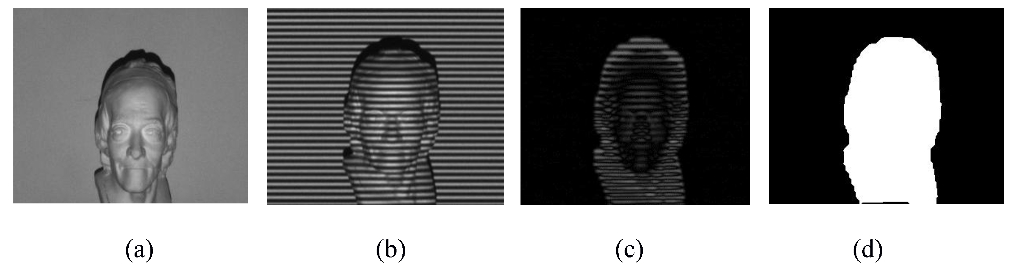
Take the Voltaire statue used in the experiment as an example to show the preprocessing of captured fringe patterns, the statue is shown as Figure 3a. And the object image with fringe patterns can be captured in three components(red component, blue component and green component) as shown in Figure 3b. After background subtraction, the calculated Figure 3c can accurately distinguish the object and the background. In order to further eliminate the effect of holes and noise, by using the morphological filter, the Figure 3d can be obtained.

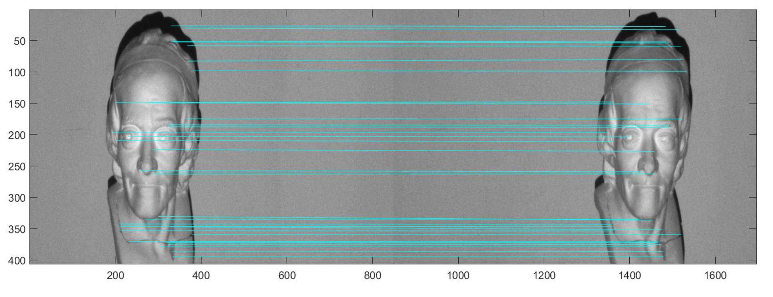
The ASIFT [30] algorithm is applied to track the object movement using the captured images with the corresponding relationship. And the output of the ASIFT algorithm is the coordinates of match points, as shown in Figure 4. According to the coordinates of match points, the corresponding relationship can also found.

4.1. Quantitative Experiments Based on Computational Performance

This experiment discusses the performance comparison of the two methods at different projection frequencies. In order to quantify the difference in accuracy of the two methods, we first compared the phase compensation results of different methods with different preset deformed phase. When the projection frequency is $30$ Hz, the compensation results of different methods are shown in

Table 1. Phase compensation results of different methods.

Method	Preset Deformed Phase (${}^{\circ }$)
	0	10	20	30	40	50
method in Ref. [16] (${}^{\circ }$)	$0.9322$	$11.0005$	$21.3034$	$31.0420$	$41.3998$	$51.0328$
Our method (${}^{\circ }$)	$1.2211$	$11.4410$	$20.9574$	$30.2873$	$40.6716$	$50.9693$
	60	70	80	90	100	110
method in Ref. [16] (${}^{\circ }$)	$61.3550$	$71.2935$	$80.9131$	$90.5499$	$100.3419$	$110.3698$
Our method (${}^{\circ }$)	$62.1627$	$71.7829$	$81.0582$	$91.3023$	$101.4257$	$111.8201$
	120	130	140	150	160	170
method in Ref. [16] (${}^{\circ }$)	$120.0243$	$130.4847$	$140.5074$	$150.4744$	$160.3691$	$170.1656$
Our method (${}^{\circ }$)	$120.8163$	$130.9091$	$140.5823$	$151.1774$	$160.4379$	$170.4528$
	180	190	200	210	220	230
method in Ref. [16] (${}^{\circ }$)	$180.0487$	$189.5176$	$200.1042$	$209.5452$	$219.5894$	$229.3869$
Our method (${}^{\circ }$)	$180.3607$	$189.5218$	$200.5750$	$210.9659$	$220.6261$	$230.2743$
	240	250	260	270	280	290
method in Ref. [16] (${}^{\circ }$)	$238.8631$	$249.1729$	$258.6368$	$268.7223$	$279.1238$	$288.9783$
Our method (${}^{\circ }$)	$239.1686$	$250.1688$	$258.9183$	$269.6454$	$279.5191$	$288.9242$
	300	310	320	330	340	350
method in Ref. [16] (${}^{\circ }$)	$298.6066$	$308.6045$	$319.1106$	$329.4160$	$339.4323$	$349.3838$
Our method (${}^{\circ }$)	$299.0089$	$309.0647$	$319.4346$	$329.6236$	$339.4916$	$349.4996$

.

In order to quantitatively evaluate the difference in phase compensation accuracy of different methods, we use Equation (15) to calculate the mean square error (MSE) of the two methods.

$$MSE=\sqrt{\frac{{\sum }_{i=0}^{N-1}{\left(\mathrm{\Delta }{\mathsf{\Phi }}_i^{{}^{\prime }(0)}-\mathrm{\Delta }{\mathsf{\Phi }}_i^{{}^{\prime }(1)}\right)}^2}{N}}$$

(15)

where $\mathrm{\Delta }{\mathsf{\Phi }}_i^{{}^{\prime }(0)}$ is the phase compensation result of the i-th deformed fringe patterns in Ref. [16], and $\mathrm{\Delta }{\mathsf{\Phi }}_i^{{}^{\prime }(1)}$ is the phase compensation result of the i-th deformed fringe patterns in our method. As shown in

Table 2. The MSE of the two methods.

Method	Frequency (Hz)
	5	10	15	20	25	30
MSE of the two methods ${(}^{\circ })$	$0.8864$	$0.5758$	$0.4801$	$0.8342$	$0.7471$	$0.6361$

, the MSE of the phase compensation results of the two methods under different projection frequencies is controlled within $1^{\circ }$.

Next, we will compare the computational cost of the two methods for phase compensation of 36 different preset deformed phase fringe patterns, the image resolution is $948\times 604$. The results are shown in the following table (

Table 3. The calculation time of different methods.

Method	Frequency (Hz)
	5	10	15	20	25	30
method in Ref. [16] (s)	$183.2324$	$193.2366$	$190.8281$	$183.0466$	$185.6055$	$184.1551$
Our method (s)	$37.3501$	$37.2767$	$37.4151$	$37.2874$	$37.3287$	$37.5048$

):

And Table 3 shows the comparison of calculation time between two methods. And the average computational cost of the method in Ref. [16] is $5.1857$ seconds/frame, our method is $1.0378$ seconds/frame. The calculation cost of our method is only $20.0127\%$ of the calculation cost of the method in Ref. [16], which greatly reduces the calculation complexity.

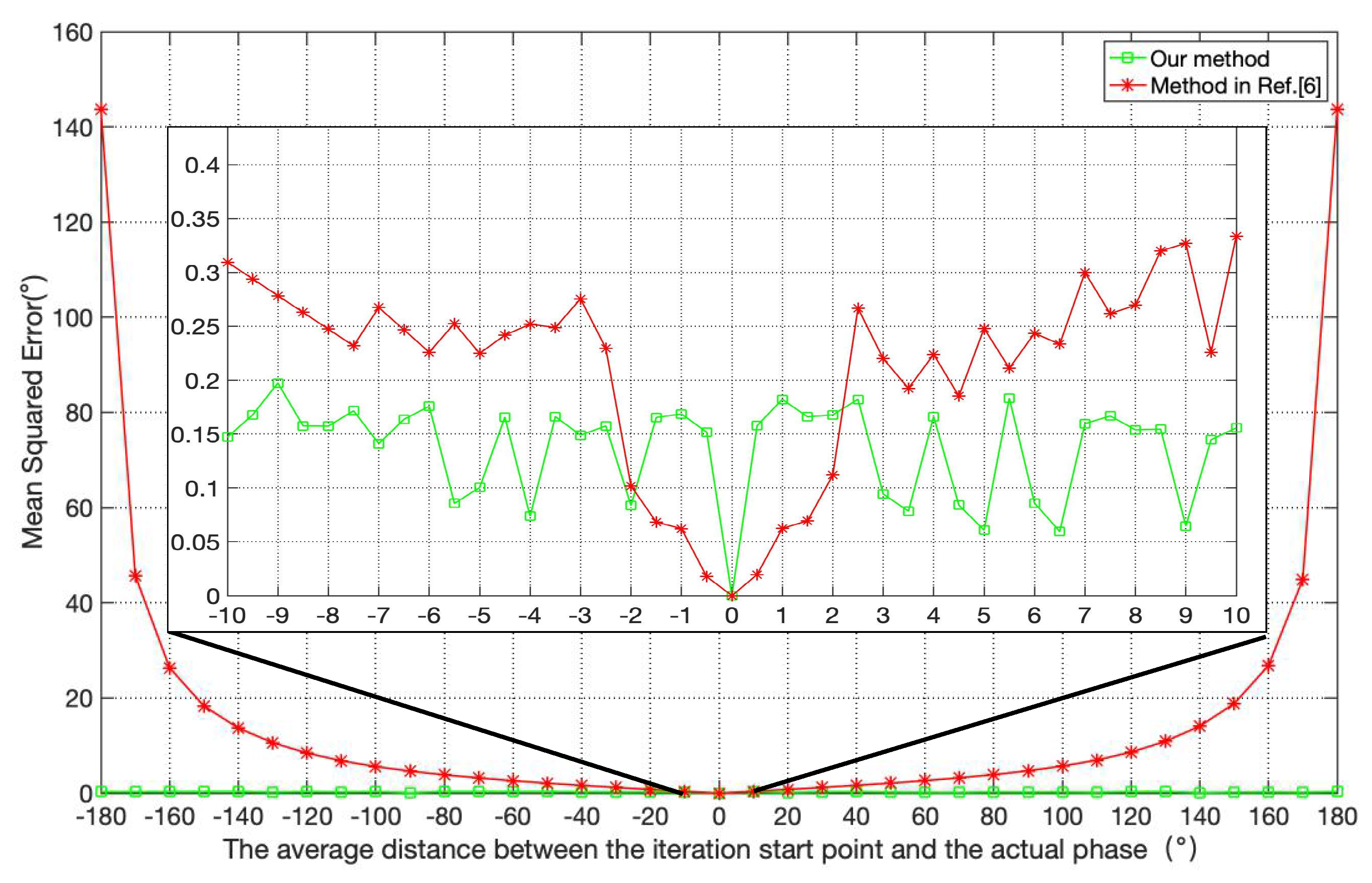
4.2. Simulation Experiment of Phase Deviation Cancellation

We selected different phase deviation within $(-\pi ,\pi )$ to verify the convergence of our method and the method in Ref. [16]. In order to facilitate quantitative analysis, we also use Equation (15) to calculate MSE between the phase compensation results and the actual phase.

At this time, $\mathrm{\Delta }{\mathsf{\Phi }}_i^{{}^{\prime }(0)}$ is the phase compensation result of the i-th deformed fringe patterns, $\mathrm{\Delta }{\mathsf{\Phi }}_i^{{}^{\prime }(1)}$ is the actual phase of the i-th deformed fringe patterns. And we assume that $\theta$ is the phase deviation, which can be calculated by the difference between the iteration starting point $\mathrm{\Delta }{\mathsf{\Phi }}_i^{{}^{\prime }(0)}$ and the actual phase $\mathrm{\Delta }{\mathsf{\Phi }}_i^{{}^{\prime }(1)}$.

When frequency is $30$ Hz, we set the $\theta =\{-{180}^{\circ },-{170}^{\circ },-{160}^{\circ },\dots ,{160}^{\circ },{170}^{\circ },{180}^{\circ }\}$. The original result is shown in the Figure 5. In order to further illustrate the effect in details, we conducted an experiment where $\theta \in [-{10}^{\circ },{10}^{\circ }]$.

It can be seen from Figure 5 that our method can converge to the actual phase at different iteration starting points within $(-\pi ,\pi )$. The MSE of our method is always controlled within $0.4^{\circ }$ and the average MSE is $0.{2437}^{\circ }$. As $\theta$ increases, the MSE of the method in Ref. [16] expands rapidly, indicating that this method is easy to fall into the local iterative optima. In the partial enlarged view, the MSE of our method is always controlled within $0.2^{\circ }$, and the average MSE is $0.{1370}^{\circ }$. When $\theta \in [-2^{\circ },2^{\circ }]$, the method in Ref. [16] is more accurate because we greatly reduce the computational complexity while sacrificing part of the accuracy. And the MSE between two methods does not exceed $0.{12}^{\circ }$. Once it exceeds this range, the MSE of the method in Ref. [16] increases with the increase of $\theta$.

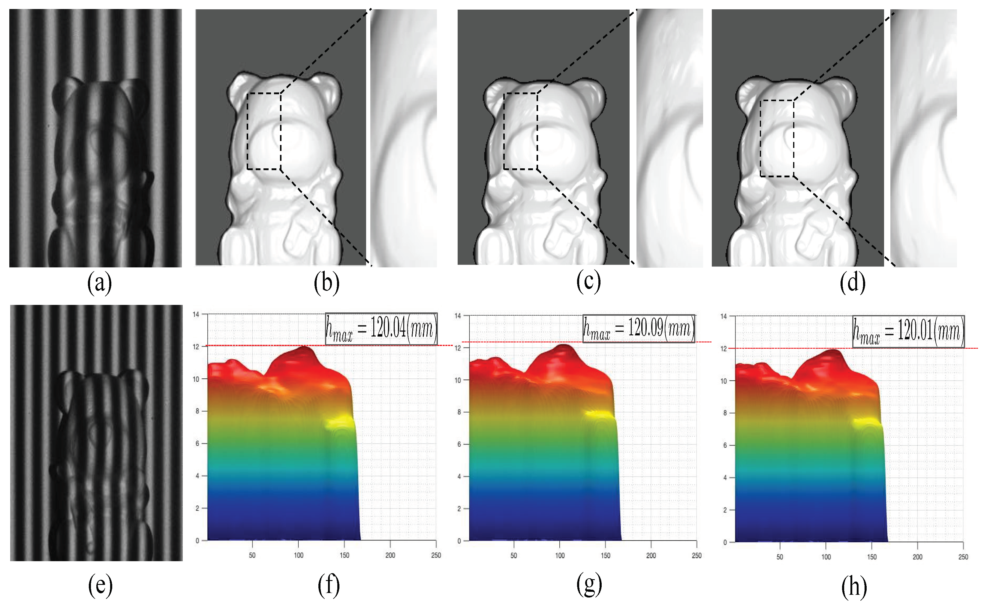
4.3. Quantitative Experiment of Free-Moving Object

We applied the proposed method to the 3D surface reconstruction of scenarios where the object is moving or stationary. For the bear statue that moves along the y-axis, we make the moving length uncontrolled each step. The surface reconstruction results of our method in different scenes are shown in Figure 6. The object moves at 3 (mm/step) between the first two fringe patterns taken, and at 5 (mm/step) between the last two fringe patterns taken. As shown in Figure 6, the proposed method has better performance in terms of details.

Due to the insignificant shape error assessment (in mm), we introduce average pixel difference ($APD$) to calculate difference between the reconstruction results of different scenarios:

$$APD=\frac{1}{h_{s,max}}\sqrt{\frac{{\sum }_{i=1}^X{\sum }_{j=1}^Y{(h_d(i,j)-h_{s,max}(i,j))}^2}{|x_{max}-x_{min}|·|y_{max}-y_{min}|}}$$

(16)

where $h_d$ is the height of surface reconstruction result in dynamic scene; $h_s$ is the height of our surface reconstruction result in static scene; $h_{s,max}$ is the height of the highest point of surface reconstruction result in static scene (i.e., the highest point of the nose of the Voltaire statue or bear statue); $x_{min}$ and $x_{max}$ are the minimum and maximum points of reconstruction result projected onto the x-axis, which are the x coordinates of the leftmost and rightmost points of the object; similarly, $y_{min}$ and $y_{max}$ are the minimum and maximum points of reconstruction result projected onto the y-axis; $APD$ shows the proportion of the error to the whole reconstruction result and further illustrates the reconstruction quality.

Calculated by Equation (16), $APD$$=5.4896\%$. If we exclude the effect of cavity area caused by changes in light and shadow, $APD$$=1.4205\%$, which means that the gap between the surface reconstruction results of moving objects and static objects is controlled in $0.1\%$.

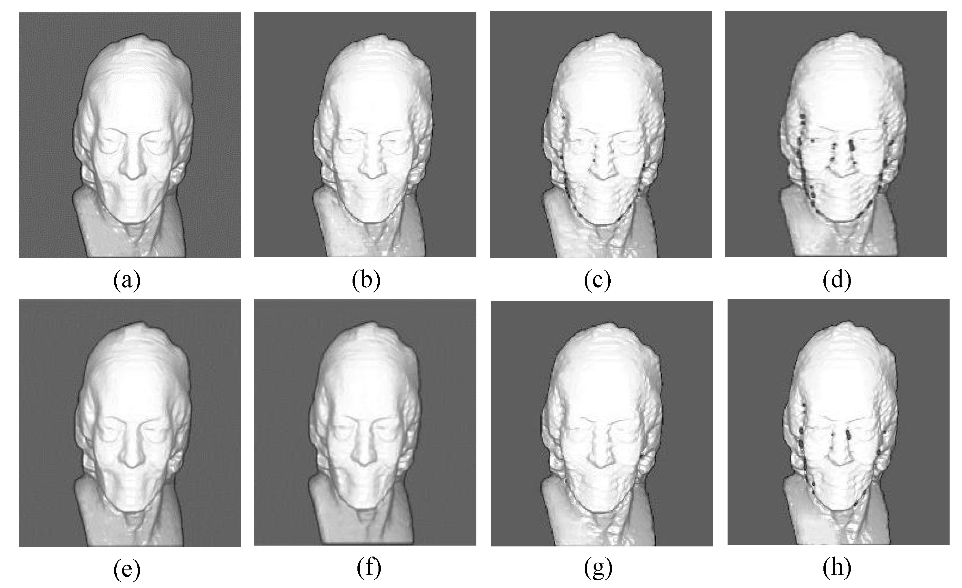
4.4. Quantitative Experiment of Different Speed

We verify the effectiveness of the proposed method by further expanding moving distance in each step and changing the movement direction of the object to the x-axis. The model used in the experiment and captured fringe pattern are shown in Figure 3a,b. The reconstruction results from traditional PSP [29] are shown in Figure 7a–d, and the reconstruction result from proposed method are shown in Figure 7e–h.

It can be seen intuitively that with the continuous expansion of the motion step length, the quality of the reconstruction result gradually deteriorates, which is caused by the limited shooting frame rate and viewing angle of the industrial camera used in the experiment. When the object is stationary and moving with a step length of 10 (mm/step), the difference between our method and traditional PSP in the reconstruction results is not intuitive.

In order to further illustrate the reconstruction quality, we use Equation (16) to calculate $APD$, which indicates difference between different reconstruction results for each motion step, and the results are shown in

Table 4. The APDs of reconstruction results with different motion steps.

Method	Motion Step (mm/step)
	0	10	20	30
Traditional PSP method	$0.0000$	$2.3860$	$4.4095$	$4.5851$
Our method	$0.0000$	$1.4045$	$2.5108$	$3.8553$

. As the motion step is expanded to 20 (mm/step), the reconstruction result of traditional method produces obvious errors in the contours of the statue, and our method still maintains good performance. When the motion step is expanded to 30 (mm/step), the distance between the initial position and the final position of the object has reached $30(N-1)$ mm while using N-step PSP. When the range of motion is expanded, the fringe patterns captured at different positions will have the perspective difference shown in Figure 7, which will lead to the information loss during the reconstruction of complex objects, such as the facial contours and nose of the Voltaire statue. If the motion step length needs to be further expanded, the camera and projection hardware used in experiments must be upgraded.

Since the shooting frame rate of the industrial camera used in the experiment is 30 frames per second, the object movement speed allowed by the experimental hardware is 400 mm/s, which can already meet the requirements of the measurement scene on the industrial assembly lines.

5. Discussion

With the idea of employing object tracking to reconstruct moving objects, one of the highlights of this paper is to significantly reduce the computational burden of traditional pixel-level phase correction methods [16]. On the other hand, the Hilbert transform-based methods [17,20] employ the Hilbert transform to shift the phase information. We will compare the object tracking-based approach with the Hilbert transform-based approach (at the principle level and in terms of performance) in future work.

Another highlight of this paper is the ability to maintain good performance even when the motion range is extended. The commonly used iterative methods are highly sensitive to the initial values and can not maintain good performance when the motion introduces large phase changes. Therefore, we redefine the iterative process and introduce an exploration mechanism to change the direction of gradient descent to find the global optimal solution and avoid getting trapped in a local optimum. With the introduction of the SGD algorithm, we have greatly improved the robustness of the method, which has been demonstrated by simulation experiments and practical experiments.

6. Conclusions

In this paper, an image-level phase compensation method in N-step PSP is presented to solve the phase deviation caused by motion. The difference among the deformed fringe patterns is introduced to construct iterative expression, which can significantly reduce the computational burden. The proposed algorithm adopts the SGD method to avoid falling into the local optima and extends the phase deviation range over existing methods. Experiments prove that the proposed method is effective when the object uses different speeds for 2-D movement. The proposed method uses a smaller time cost to achieve a larger allowable range of motion, and achieves a balance between computational complexity and algorithm effective range.