Evolutionary Strategy for Practical Design of Passive Optical Networks

Abstract

Passive optical networks (PONs) are an important and interesting technology for broadband access as a result of the growing demand for bandwidth over the past 10 years. An arduous and complex step in the design of such networks involves determining the placement of equipment, optical fiber cables and several other parameters relevant to the proper functioning of the network. In this paper, we propose an evolutionary strategy to optimize the infrastructure design of PONs by using genetic algorithm technique. This meta-heuristic is capable of elaborating fast, automatic and efficient solutions for the design and planning of PONs. Our proposal has been developed using real maps, aiming to minimize deployment costs and time spent to carry out PON projects, achieving pre-defined quality criteria. We considered, in our simulations, two scenarios (non-dense and dense), four possible topologies and two regions of interest. The non-dense consists of a scenario in which subscribers are distributed in a dispersed manner in the region of interest. The dense has a considerably higher number of subscribers distributed in a very close way to each other. Based on the obtained results, the potential of our proposal is quite clear, as well as its relevance from a technical, economic, and commercial point of view.

1. Introduction

The emergence of new services using the Internet (applications such as video-on-demand, 3D high-definition television (TV), 4K, or 8K ultra-high definition (UHD), machine-to-machine (M2M), cloud computing, virtual/augmented reality (VR/AR) and fifth-generation mobile network (5G), for example) will require optical networks to transport traffic with different values of quality-of-service (QoS) and bandwidth requirements [1,2,3]. As reported by Cisco Systems [4], the number of global Internet users will be $5.3$ billion (66% of the global population) by 2023. Fixed broadband speeds will be more than double by 2023. By 2023, global fixed broadband speeds will reach $110.4$ Mbps, up from $45.9$ Mbps in 2018. According to Federal Communications Commission’s (FCC) broadband guide [5], a common house with regularly simultaneous uses of two or three devices, using applications that require basic or moderate traffic (e.g., email, browsing, video, voice-over-internet protocol (VoIP) and at least one streaming HD video or an online gaming application), requires a service that offers a bandwidth of 12 to 25 Mbps. As a result, the consumer’s demands may not be satisfactorily met if a high-quality access network service is not available in the subscriber’s region.

Broadband services have traditionally been provided over digital line subscriber (DSL) or cable modem networks [6]. However, it becomes even harder to support the fast-growing demand of users due to the fundamental bandwidth limitations of copper-based networks [7]. As a result, technologies based on optical fiber emerge as an alternative to meet these demands and the high quality-of-service required in access networks [8]. According to the Brazilian National Telecommunications Agency (ANATEL) report [9], in August 2019, approximately $65.2$% of the Brazilian’s access networks were still based on copper cables. However, it is worth mentioning the recent growth in the use of optical fiber (reaching the percentage of $26.3$% on the same date). Another relevant piece of data is that only $46.7$% of Brazilian households have fixed broadband access, which means that the optical fiber access network services will grow in the next few years.

Several fiber access network architectures have been developed (e.g., point-to-point, active optical network and passive optical network) [10]. However, passive optical networks (PONs) stand out. A passive optical network means that it does not need electrical power in the outside plant. PONs’ advantages include [11]: easy installation and updating; low cost of operation and maintenance; high reliability, electromagnetic immunity; and compact size cables. Nowadays, PONs have been launched into the practical market with Gigabit-capable PON (GPON), and following on from this, with its next generations XGS-PON and HS-PON (which are already standardized by ITU-T). Their ITU-T recommendations containing all technicals details are available in [12,13,14]. It should be noted that network designers and planners are therefore faced with several key challenges at all stages of the design process and this is not always an easy task, as many possibilities exist [15]. Thus, the PONs planning task can require several days to be completed, wasting resources that could be allocated to other assignment and demands.

In this paper we propose an algorithm for PON planning based on the use of genetic algorithm (GA) technique. By using basic information such as streets, avenues, central office (CO) position, subscriber location and four possible topologies, the proposed algorithm finds a solution to the PON planning problem, considering four possible topologies in two simulation scenarios (non-dense and dense) and two different regions of interest. In the non-dense scenario, subscribers are distributed in a dispersed manner in the region of interest. The dense scenario has a considerably higher number of subscribers distributed very close to each other. The objective is to minimize the network deployment cost, as well as reduce the time spent to find the problem solution. In addition, we explain in detail the capital expenditure (Capex) model, concepts of graphs theory used by our proposed algorithm for PONs planning optimization, the process of importing maps in real time and the optical power budget. This paper is organized as follows: In Section 2, the problem characterization is discussed. In Section 3, we present the four possible topologies adopted in our simulations. In Section 4, our proposed algorithm for PON optimization and, in Section 5, the simulation scenarios considered in this paper are described in detail. In Section 6, the results are discussed and, finally, in Section 7, we present the conclusions.

2. Discussion

There are numerous optical network technologies. However, PON stands out by offering a highly efficient and cost-effective access network [1]. A PON’s main feature is that it is implemented as a point-to-multipoint architecture, in which unpowered fiber optic splitters are used to enable a single optical fiber to serve multiple end-points (consumers) [16]. Due to the consideration of many design factors, the optical network planning process often exhibits several challenges from the optimization point of view [17,18]. To design a cost-effective PON, it is required the consideration of many factors such as the split ratio, position of optical splitters in the optical distribution network (ODN) and the assignment of subscriber premises to the splitters. In addition, all the planning rules must be satisfied including constraints on equipment capacity and the maximum cabling distances which are derived from power budget constraints [19]. For this purpose, several optimization techniques have been used for access network planning in order to find an efficient infrastructure to meet requirements, aiming to obtain the lowest possible deployment cost [20]. Nowadays, network planning is one of the most important topics of PONs. Therefore, several proposals based on mathematical techniques, heuristic and meta-heuristic algorithms have been reported for this optimization problem [18,20,21,22].

Chu et al. [18] proposed a heuristic algorithm based on ant colony optimization (ACO) to minimize the PON deployment cost. In summary, the ACO algorithm is a probabilistic technique for solving computational problems. This technique is inspired by the behavior of ants that leave their nest seeking the shortest path between their colony and a source of food. Chu et al. [18] developed a system that was able to minimize the PON deployment for a specific tree PON topology. The considered topology was limited to use just one level of optical splitters and drop closures for the distribution of optical fibers. The objective function was based on the deployment network cost. In addition, when the cost was evaluated, only optical cables, optical splitters and drop closures were considered, ignoring others important deployment costs such as optical splices, network elements in central office, etc. However, Chu et al. [18] do not inform how the obtained results were validated. Regarding the adopted scenarios for the tests, the authors informed only that they were based on real scenarios, but did not present used maps and neither inform more details about them.

Pehnelt et al. [20] proposed an algorithm which deals with optimization of PON designs. The proposed system used a combination of different methods to find the solutions. Firstly, Pehnelt et al. [20] introduced an algorithm based on Dijkstra’s algorithm to find optimum (minimum) distances between optical line terminals (OLT) and optical network terminals (ONT). Then, for the second part (optimum splitter placement), k-mean clustering and hierarchical clustering techniques were used. The proposed algorithm found an optimal metric, thus creating the optimized tree topology mainly focused on summary trenching distance (although endpoint attenuation and minimum summary length of optical fibers were considered). For tests, it was used a real map of a small residential neighborhood of Prague (Czech Republic). Raw data were obtained from Open Street Maps (OSMs) software. For simulations, a scenarios using 40 ONTs and one single OLT, randomly placed on the map, using one to three levels of optical splitters in the outside plant was considered. The proposed algorithm was a good alternative to conventional methods and the results were presented in graphical and table forms. However, important parameters that also influence the deployment cost were not considered (such as splices, cabinets, etc.) and only one type of cable was used for the entire network. The tested scenario considered by Pehnelt et al. [20] was relatively small, which greatly reduces the search space and simplifies the task of finding the optimal solution.

Villalba et al. [21] proposed a genetic algorithm for solving PONs projects considering three different types of basic topologies, such as tree, ring and bus. The proposed GA was responsible for determining the optical splitters’ placement in the network and also the optical cables’ routing, seeking for the lowest cost of implanting the network. However, despite presenting a good performance when compared to manual methods, the developed tool was quite simple and considered only the splitters cost and the cost of a single type of cable, not taking into account several other factors involved in proper network planning. In [21], the used maps were not georeferenced and no further details were provided on the process of importing the maps.

Eira et al. [22] introduced an integer linear programming (ILP) model which was capable of designing a single-stage and multiple-stage splitting PON. In order to reduce the computation time for larger sizes, a two-stage heuristic was proposed to tackle with scenarios that were beyond the computational abilities of the optimal method. The aim of the paper was finding the least costly tree topology deployment configuration considering equipment and installation costs. For the single-stage ILP model, the authors adapted the classical concentrator location problem (CLP) applied to telecommunications network. For the multistage problem, new ILP model was formulated to deal with it. The following inputs were considered: OLT and optical network units (ONU) locations; number of candidate locations for splitter placement; and respective interconnection costs. The maximum split ratio allowed by each PON port was assumed to be 64. For the heuristic approach, developed to cope with large-scale multistage PONs, the authors proposed an algorithm that used the same inputs as the ILP model. The basic concept was to obtain an initial cost-effective configuration and then locally to search for alterations in the network layout in order to reduce the overall cost. It should be noted that power budget constraint was considered in both approaches. Although not addressed in the paper, the authors highlighted that presented approaches can be easily adapted to other PON technology types. However, in the simulations, georeferenced or real maps were not used, which provides poor details compared to a real PON planning problem. Moreover, the adopted size of the available splitters placing locations was reduced (search space). These possibilities were quite small, reaching only 50 possibilities (in the worst case), leading to a reduction in the optimization problem complexity.

Some recent works involve evaluation scenarios that are not part of the scope of this paper, such as: radio-over-fiber, internet of things and data centers. As an example, in [23], the authors present a novel radio-over-optical fiber network architecture with multi-stratum resources optimization using software-defined networking. The proposed architecture can globally optimize radio frequency, optical spectrum and cloud baseband unit processing resources effectively to maximize radio coverage and meet the quality of service requirement. In [24], the authors propose a brain-like productive service provisioning scheme with federated learning for industrial internet of things. The scheme combines production information into network optimization, and uses the interfactory and intrafactory relations to enhance the accuracy of service prediction. In [25], the authors present a novel architecture that can enable cross-stratum optimization of application and optical network stratum resources, and enhance multiple-layer resource integration in ubiquitous data center optical interconnection.

In this paper, we propose an evolutionary strategy to optimize the design of PONs. Compared to the existing approaches presented in previous papers [18,20,21,22], our proposal is simple but efficient and complete, supplying the main deficiencies found in previous papers [18,20,21,22]. The technique proposed is based on genetic algorithm and this choice is mainly due to the simplicity of its implementation and the good results obtained in problems involving graphs. In summary, the proposed algorithm in this paper aims to minimize deployment costs and time spent to make the project, using real georeferenced maps, displaying the results in a graphical, friendly and complete way. For network cost calculation, all the typical materials and services involved in GPON deployment were considered. The restrictions considered in this paper are also stricter and are based on real scenarios, which means more practical results. The efficiency of the proposed system has been validated by comparisons with manual planning of PONs (traditional way), resulting on great performance, with total cost values lower than those obtained with the traditional way. Moreover, all simulations and tests of the proposed system were performed on real maps, considering two different simulation scenarios (non-dense and dense), four GPON topologies and two regions of interest.

Table 1. Summary of the contributions of the papers available in the literature and the main characteristics of our proposal in this paper.

Item	[18]	[20]	[21]	[22]	Our Proposal
Approach	ACO	Dijkstra and k-means	GA	ILP and	GA
Georeferenced real maps	–	X	–	–	X
Number of splitters possible positions (worst available case)	5	N/A	N/A	50	714
Number of ONUs (worst available case)	1033	40	120	1000	1544
Multistage network	X	X	X	X	X
Maximum split ratio (per PON)	N/A	64	128	64	64
Elapsed time (min) (for worst available case)	4.06	N/A	N/A	N/A	72.27

describes a summary of the contributions of the papers available in the literature and the main characteristics of our proposal in this paper.

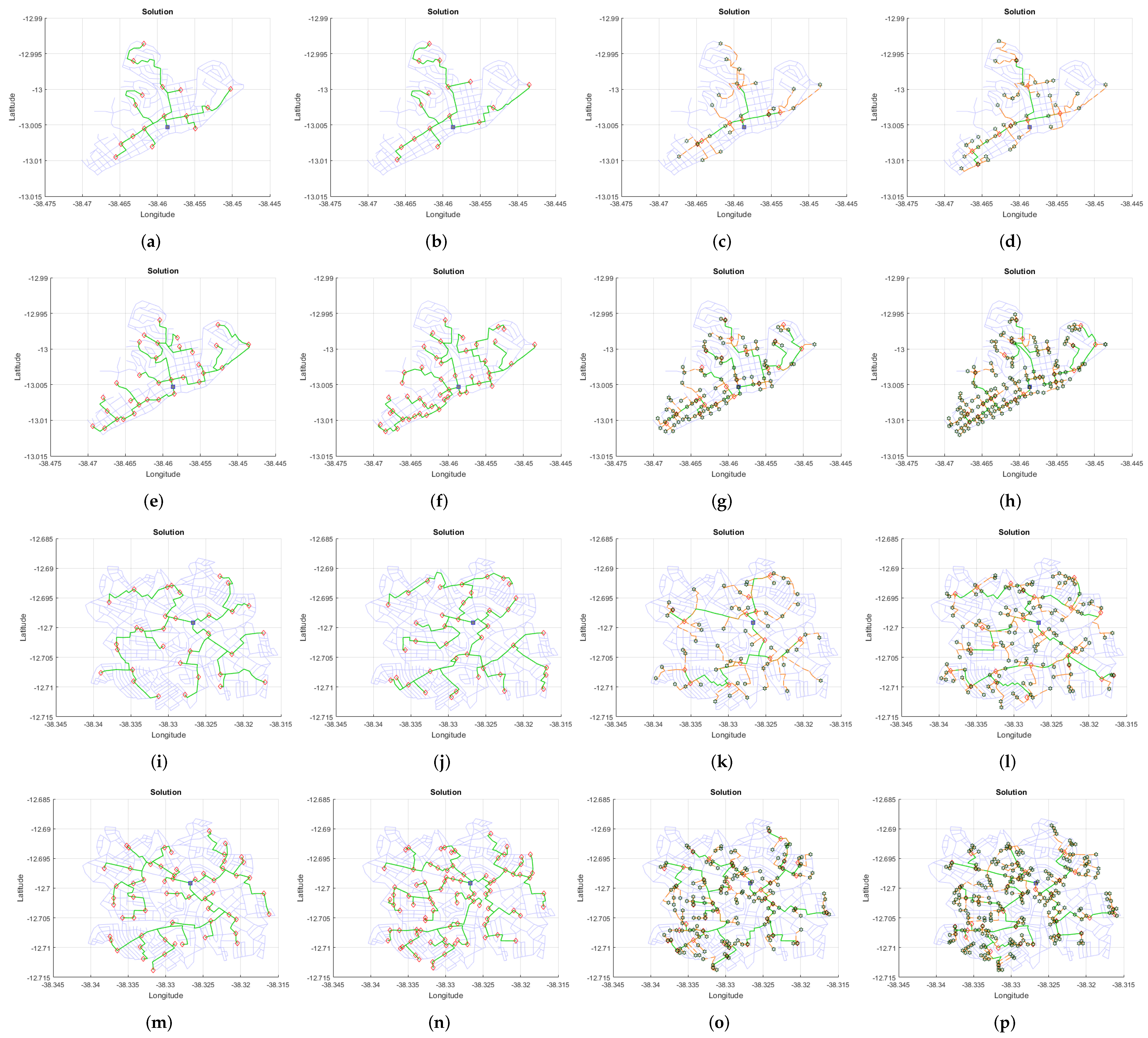
3. Adopted Topologies for Proposed Systems

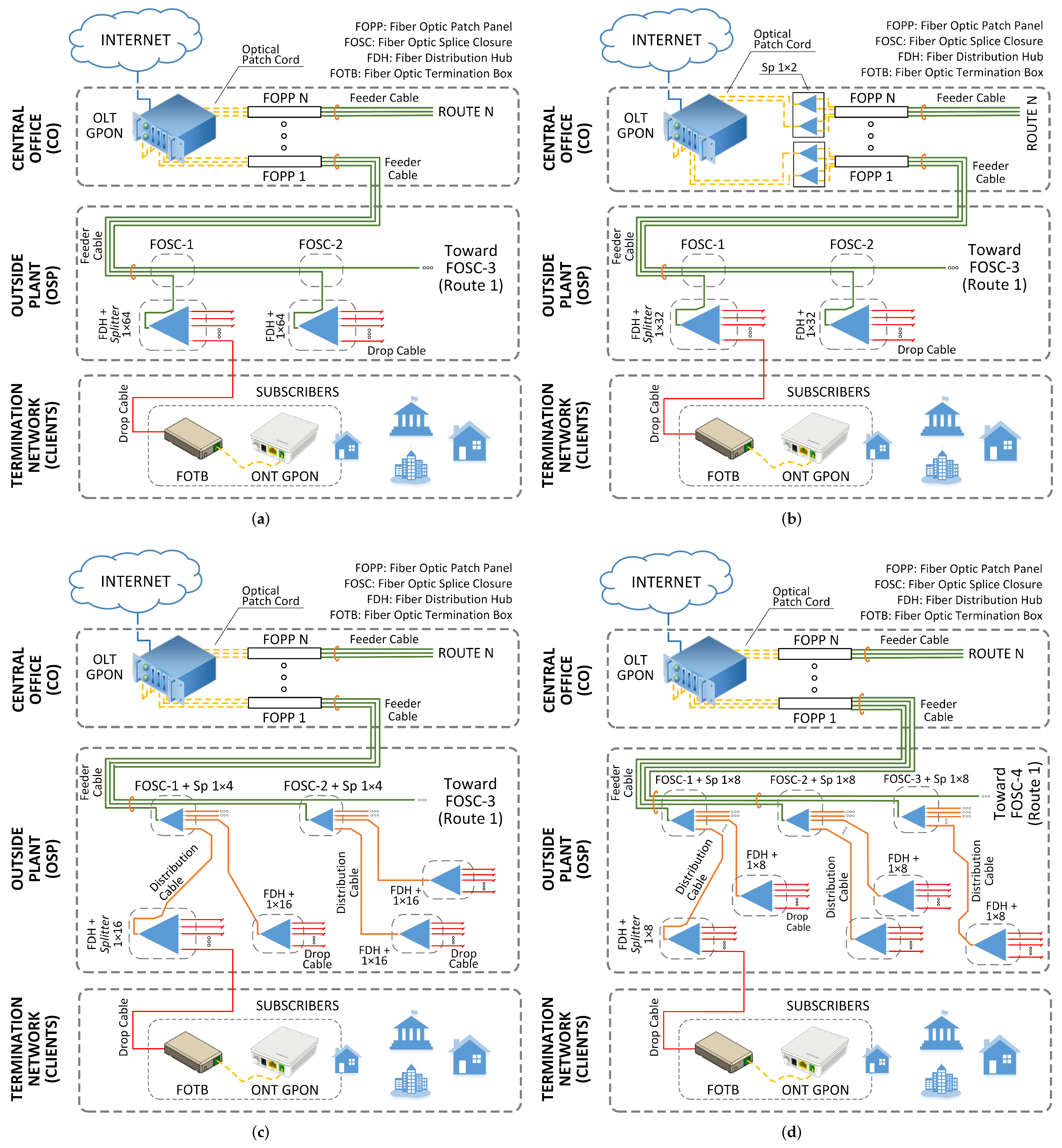
PON systems can use bus, ring, tree or a mix of these previous topologies [21]. This choice occurs at the network planning stage and each topology has different characteristics, being implemented according to the situation and requirements of each project [26]. Therefore, the appropriate topology choice depends on the project premises, such as redundancy requirement, service capillarity and how subscribers and potential subscribers will be geographically arranged.

Among the basic PON topologies, Internet service providers (ISPs) typically adopt the tree topology [27]. This is mainly due to cost reduction and greater network connectivity for subscribers who lives in a certain region [22]. However, the wide range of splitter configuration and placement possibilities create an extensive list of tree-topology types using single or multiple stages. The way the optical splitters are arranged in the network defines whether the system is composed of a centralized topology (with a single splitter stage in the outside plant) or a distributed (also known as cascated) topology (with multiple splitter stages in the outside plant) [26,28]. In general, a centralized approach typically offers lower operational costs and is easier to access and to control for technicians. On the other hand, distributed topology brings faster return-on-investment, lower initial costs and lower fiber costs [28]. This leads to a typical benefits and disadvantages trade-off decision.

It also should be highlighted that the filling rate of an OLT PON port has a direct impact on the number of OLT PON cards and the size of the OLT shelf. Consequently, it has a direct impact on the deployment cost. The way how fiber distribution hubs (FDHs) are distributed and connected in the ODN (e.g., same areas or areas with different fiber service appetites) may influence how PON cards are gradually activated or utilized. In other words, PON cards activations can be postponed or reduced based on how FDHs are inter-connected.

Although our proposal can be easily adapted for different scenarios, this paper focuses on fiber-to-the-home (FTTH) deployment planning using GPON system. For this purpose, the following topologies were considered (Section 3.1, Section 3.2, Section 3.3 and Section 3.4): (1) Centralized Topology—Type 1 (CTT1), (2) Centralized Topology—Type 2 (CTT2), (3) Distributed Topology—Type 1 (DTT1) and (4) Distributed Topology—Type 2 (DTT2). It is worth mentioning that the specifics of these hypothetical topologies are considered in order to represent a real GPON deployment using the two aforementioned approaches for tree topologies (known as centralized and distributed topologies). These topologies are commonly used by ISPs and basic concepts are described in [28]. Figure 1 shows the physical topology diagram for: (a) CTT1, (b) CTT2, (c) DTT1 and (d) DTT2, and

Table 2. Summary of considered topologies in this paper.

Topology	Topology Type Approach	Number of Splitter Stages	Adopted Split Ratio	Splitter’s Placement
CTT1	Centralized	1	1 × 64	OSP
CTT2	Centralized	2	1 × 2 and 1 × 32	CO and OSP
DTT1	Distributed	2	1 × 4 and 1 × 16	OSP
DTT2	Distributed	2	1 × 8 and 1 × 8	OSP

presents the summary of the adopted topologies in terms of topology type approach, number of splitter stages, network split ratio and splitter’s placement.

3.1. CTT1

This topology uses a single-stage splitter configuration with a split ratio of 1 × 64. This single-stage splitter is placed in an outside plant (OSP) telecommunications enclosure or cabinet. In this paper, we call this enclosure a fiber distribution hub (FDH). In comparison with other topologies, due to the high splice ratio of access splitter (1 × 64), this topology has a reduction in the number of passive network elements in the OSP. However, on the other hand, in general, FDH are installed further away from subscribers, leading to a significant increase in the length of drop cables. Figure 1a shows the physical diagram of the network when CTT1 is adopted. A feeder cable with a high amount of fibers feeds access splitters (with split rate of 1 × 64) placed at FDHs in an OSP and these splitters serve subscribers.

3.2. CTT2

This approach uses a combined split ratio of 1 × 64, with two levels of splitters, these being 1 × 2 splitters placed inside the CO and 1 × 32 splitters placed in an OSP-FDH. This topology is also considered centralized because it still only has a single-stage splitter in the OSP. In comparison with the previous presented topology (Section 3.1), an increase of FDHs is expected in the external network (due to the lower capacity of access splitter) and a greater use of fibers in the feeder cable. However, on the other hand, the tendency is a reduction in the length of drop cables (used to serve subscribers) due to the increased number of access splitters in the OSP. Figure 1b shows the physical diagram of the network when CTT2 is adopted.

3.3. DTT1

This topology uses two levels of splitters in the OSP and has no splitter in the CO. The first level of splitting is used for distribution, has a splice ratio of 1 × 4 and is installed in a fiber optic splice closure (FOSC) in the OSP. The second level of splitting is used for subscriber access, has a splice ratio of 1 × 16 and is placed in FDHs. In relation to the above-mentioned topologies (Section 3.1 and Section 3.2), a significant increase in the number of passive elements along the external network is expected, as is a reduction in the used fibers of the feeder cable. However, the tendency is a reduction in the length of drop cables used to serve subscribers once, in these topologies, FDHs will be closer to subscribers. Figure 1c shows the physical diagram of the network when DTT1 is adopted.

3.4. DTT2

This last approach also uses two levels of splitters in the OSP and has no splitters inside the CO. The first splitter (distribution splitter) has a splice ratio of 1 × 8 and is installed in a FOSC in the OSP, while the second level has other 1 × 8 splitters (access splitters) placed in FDHs. In this topology, access splitters are placed very close to subscribers, leading to a great reduction in drop cable length. However, on the other hand, among considered topologies in this paper (Section 3.1 and Section 3.3), this one has a higher number of passive network components in the OSP. Figure 1d shows the physical diagram of the network when DTT2 is adopted.

4. Proposed Algorithm for PON Optimization

For the mathematical representation of the region, in which a PON is planned and optimized (region of interest), the elementary concepts of graphs theory were used. These concepts are discussed in details in Section 4.1. In Section 4.2, some basic aspects of genetic algorithm and, in Section 4.3, our proposed GA are presented.

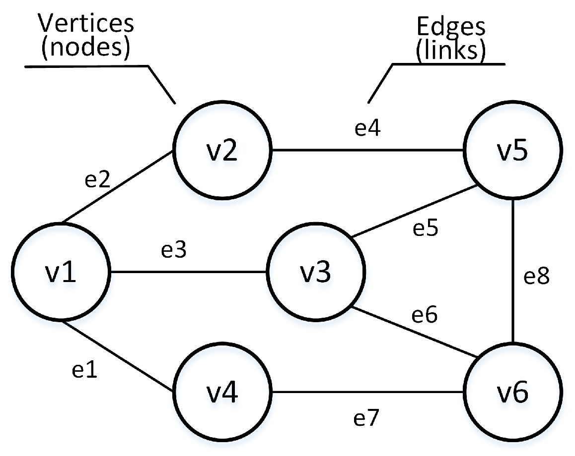
4.1. Theory of Graphs

Graphs are an important mathematical tool and have been widely used to represent problems in the most diverse areas of knowledge [29]. They can reproduce any network, such as a telecommunications network [29]. Figure 2 shows a simple, non-oriented graph, in which V represents vertices (or nodes) and E represents edges (or links).

One of the most simple way to represent a graph mathematically is through the use of adjacency matrices. These matrices describe how vertices of the graph are connected. In general, given a graph with V vertices (nodes), it can be represented using a matrix A of dimension $V\times V$. For the representation of non-directed graphs without weights at the edges, each value of matrix A can be defined by

$$a_{i,j}=\left\{\begin{array}{l}1,\mathrm{if}\mathrm{vertices}{v}_i\mathrm{and}{v}_j\mathrm{are}\mathrm{adjacents};\\ 0,\mathrm{otherwise}.\end{array}\right.$$

(1)

It is then noted that a binary matrix is formed for this case. If the edges have associated weights, the entered value for $a_{ij}$ will have, instead of 1, the numeric value associated with the edge. To illustrate, the graph shown in Figure 2 is represented by the following adjacency matrix (A) (without weights)

$$A=\left[\begin{array}{cccccc}0& 1& 1& 1& 0& 0\\ 1& 0& 0& 0& 1& 0\\ 1& 0& 0& 0& 1& 1\\ 1& 0& 0& 0& 0& 1\\ 0& 1& 1& 0& 0& 1\\ 0& 0& 1& 1& 1& 0\end{array}\right].$$

(2)

It should be emphasized that the use of graphs as a tool for map representation is very common in the literature. The graphs are used to describe the PONs design problem. In general, corners can be represented by vertices, edges can represent streets and avenues, and weights (of each edge) are distances between two vertices [20,21,27].

4.2. Genetic Algorithm

The first research on GAs was developed and published by John Holland [30]. Since then, genetic algorithms have been successfully applied to a wide range of optimization and machine learning problems, including the optimization of PONs planning [21].

Initially, when a GA is executed, P individuals are generated randomly and each individual represents a possible solution to the problem. Each individual is composed of chromosomes and these are represented by a set of genes. As a further process of the algorithm, this set of individuals (population) is evaluated by using a fitness function. The better-fitting individuals are selected from the current population, and unfitted individuals are discarded. From this point on, the selected individuals have their genes modified through genetic operators known as crossover and mutation. The new generation of possible solutions is then used in the next iteration of the algorithm. This cycle is repeated until an appropriate solution is found or the number of interactions (generations), previously defined, is reached. The main goal of this technique is to find the individual that most fit the environment during the evolution process [31].

One of the greatest advantages of GAs is the simplicity in the optimization problem formulation [32]. Usually, fixed-length bit strings are used as input for the algorithm, which perfectly adapts to problems involving graphs [33,34,35]. Another advantage is the fast convergence time, in comparison to polynomial algorithms, for problems that involve a large number of variables [36]. Although GA is an algorithm that usually presents robust results, as it is a meta-heuristic method, the solution can converge to a local minimum, presenting a false optimal response. However, this premature convergence can be minimized with an appropriate adjustment in the number of generations, population size and genetic operators [37,38].

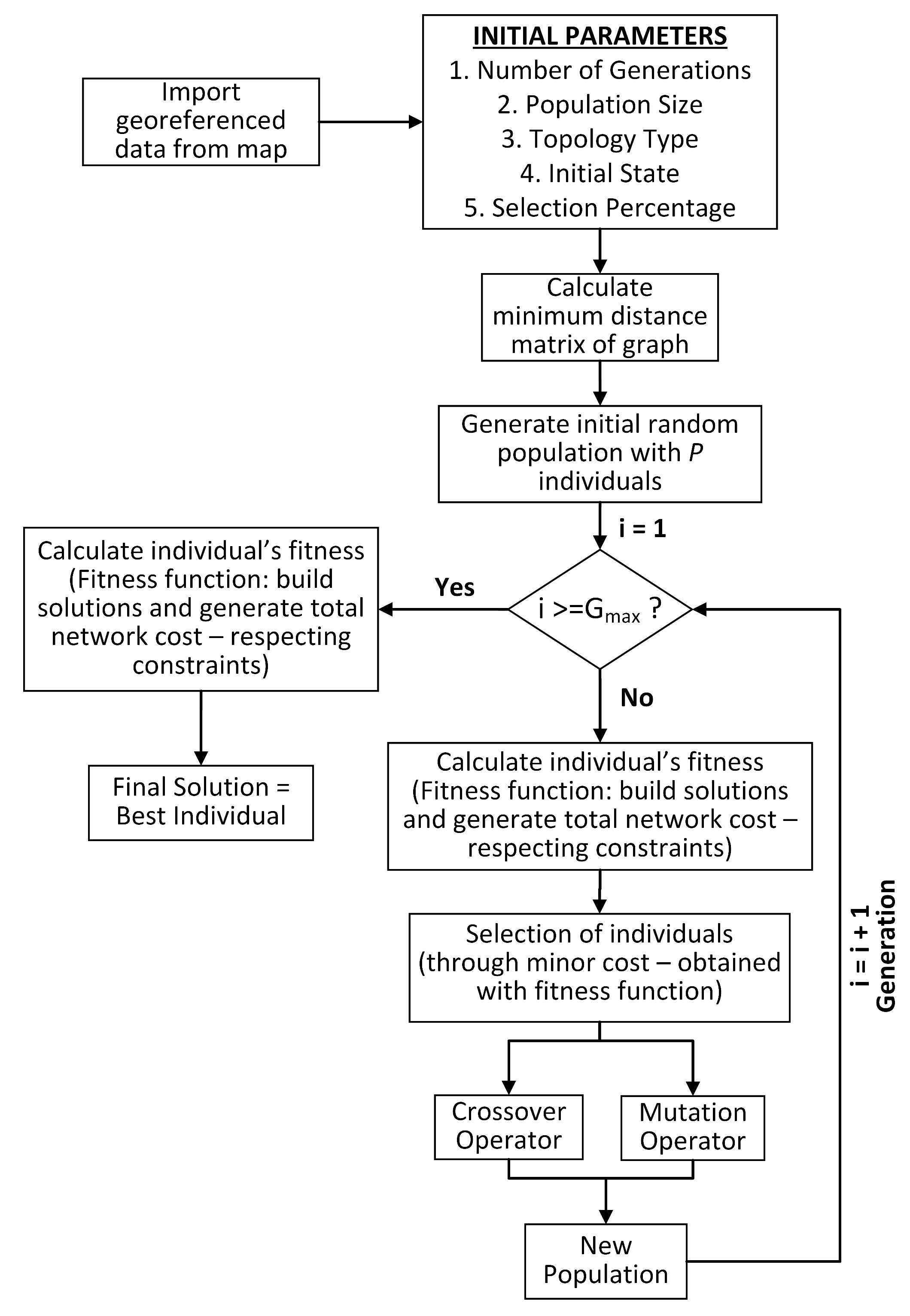
4.3. Our Proposed Genetic Algorithm for Optimization of PONs Planning

Figure 3 shows the flowchart of our proposed genetic algorithm for optimization of PONs planning. The algorithm can be represented by the following steps:

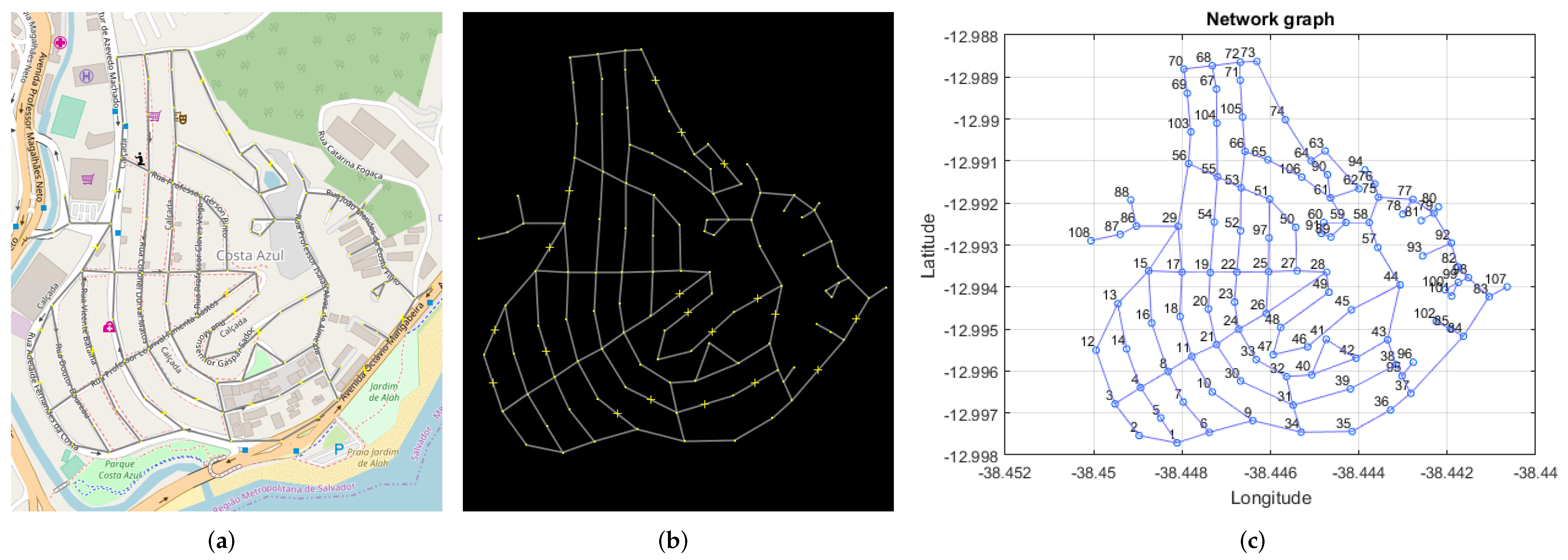
• (1) Import the georeferencing data obtained from the map: In this step, the georeferenced data of the region of interest is imported to Matlab^®. OSM software is used to obtain the region’s raw data. The region of interest is selected and, in the file exported by the OSM, the intersections between streets (corners) are identified with global position system (GPS), as well as the links among those intersections. These raw data (.xml file) are then imported into Matlab^® and a georeferenced graph of the region of interest is created. The weight of each edge of the graph’s adjacency matrix is the calculated distance (in meters) among the network nodes. Figure 4 shows a graphical example of importing georeferenced data to Matlab^®, considering: (a) example of a region of interest (Costa Azul neighborhood, Salvador city, Brazil) with overlapping graph; (b) example of a region of interest to be imported into Matlab^®; and (c) network graph, containing 108 nodes, imported to Matlab^®.
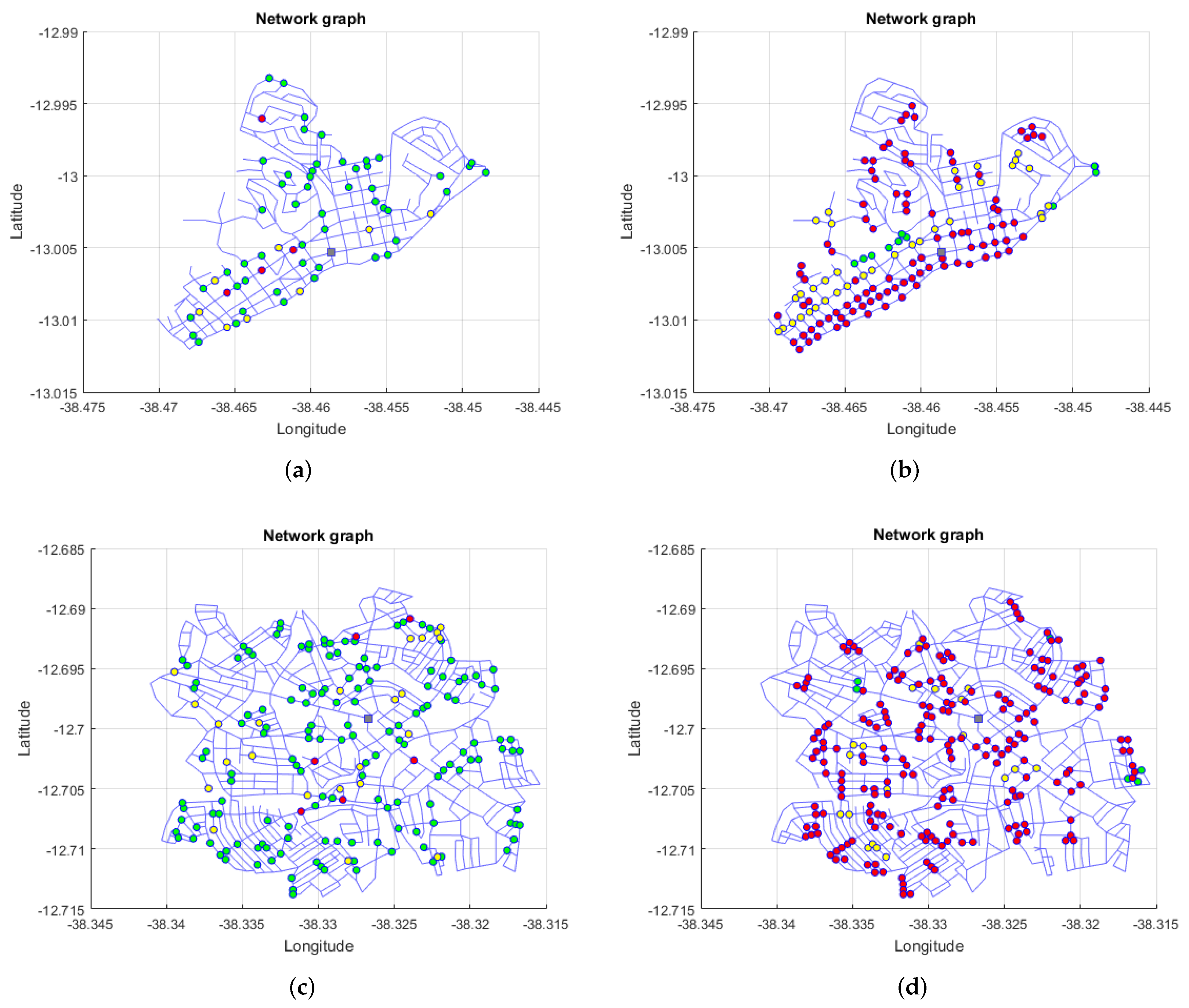
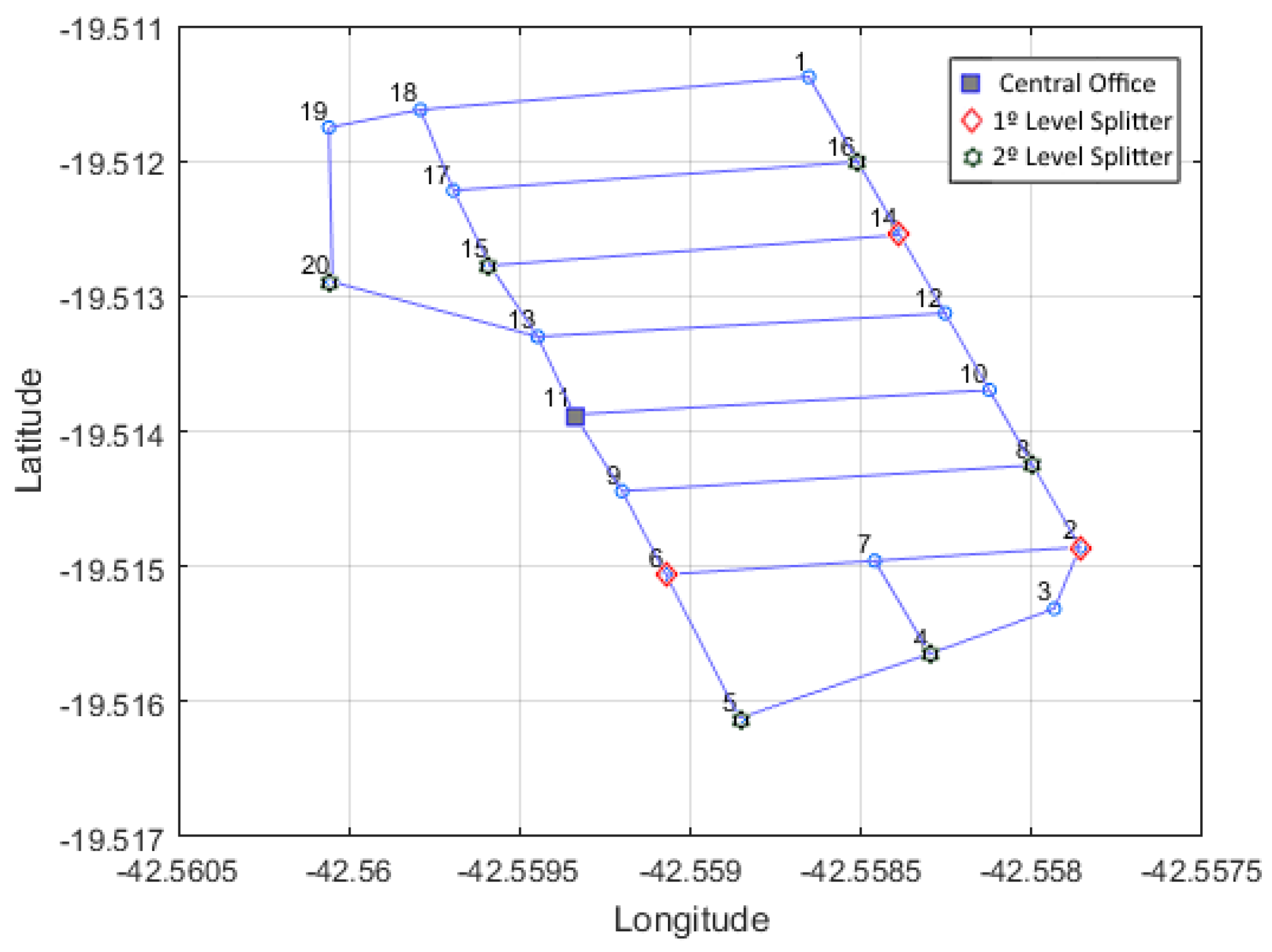
• (2) Set initial parameters: here, initial parameters must be defined. These parameters are:
  ($2.1$) Number of generations: defines how many iterations the GA will run;
  ($2.2$) Population size: defines the number of individuals of each GA generation;
  ($2.3$) Topology type: defines the topology (one of the four possible topologies described in Section 3);
  ($2.4$) Initial state: Defines the position of each potential subscriber in the respective scenario. Subscriber positions are represented by a matrix of $N\times M$, where N is 1 and M is the map graph dimension. Each value of the matrix will be the number of subscribers in that specific node. In this paper, we defined as possibility only two, four or seven subscribers. In this stage, we also set the location of the CO using another matrix $N\times M$. In the matrix, the node position holding the CO is set to 1 while other positions are set to 0. Figure 5 shows examples of initial states used as input of our simulations (as can be seen in Section 6). Green, yellow and red nodes represent, respectively: two, four and seven subscribers on the node;
  ($2.5$) Selection percentage: Defines the number of most fit individuals (in %) who will participate to the subsequent steps (genetic operators—crossover and mutation) in each generation.
• (3) Calculate the minimum graph distance matrix: Using the obtained data in the previous step (step 1), the algorithm performs the calculation of the graph minimum distance matrix, using a well-known Floyd–Warshall algorithm [39]. The choice of this algorithm is due to the good performance and simplicity of its implementation. The minimum distance matrix is $M\times M$ (in which M is the graph dimension) and contains the minimum distances (in meters) among all graph nodes.
• (4) Generate the initial population randomly with P individuals: In this step, a set of P random individuals is generated, allowing a wide range of possible initial solutions. Each individual will be represented by a line in the population matrix. This matrix will be $P\times M$, in which P is the population size and M is the graph dimension. In addition, each gene (of the individuals) represents one possible node position for optical splitters in the network graph. Thus, each individual represents a possible solution to the problem. It is worth mentioning that topologies with two splitting stages will be represented with two population matrices (each one for each splitting level). The following matrices ($A_1$ and $A_2$) represent a random initial population for an hypothetical scenario of a PON using two splitter stage. Figure 6 represents graphically the first individual of both matrices.

  $$A_1=\left[\begin{array}{cccccccccc}0& 1& 0& 0& 0& 1& 0& 0& \cdots & 0\\ ⋮& ⋮& ⋮& ⋮& ⋮& ⋮& ⋮& ⋮& \ddots & ⋮\\ 0& 0& 0& 1& 0& 0& 1& 0& \cdots & 0\end{array}\right],$$

  (3)

  $$A_2=\left[\begin{array}{cccccccccc}0& 0& 0& 1& 1& 0& 0& 1& \cdots & 1\\ ⋮& ⋮& ⋮& ⋮& ⋮& ⋮& ⋮& ⋮& \ddots & ⋮\\ 0& 1& 0& 1& 1& 0& 0& 0& \cdots & 0\end{array}\right].$$

  (4)
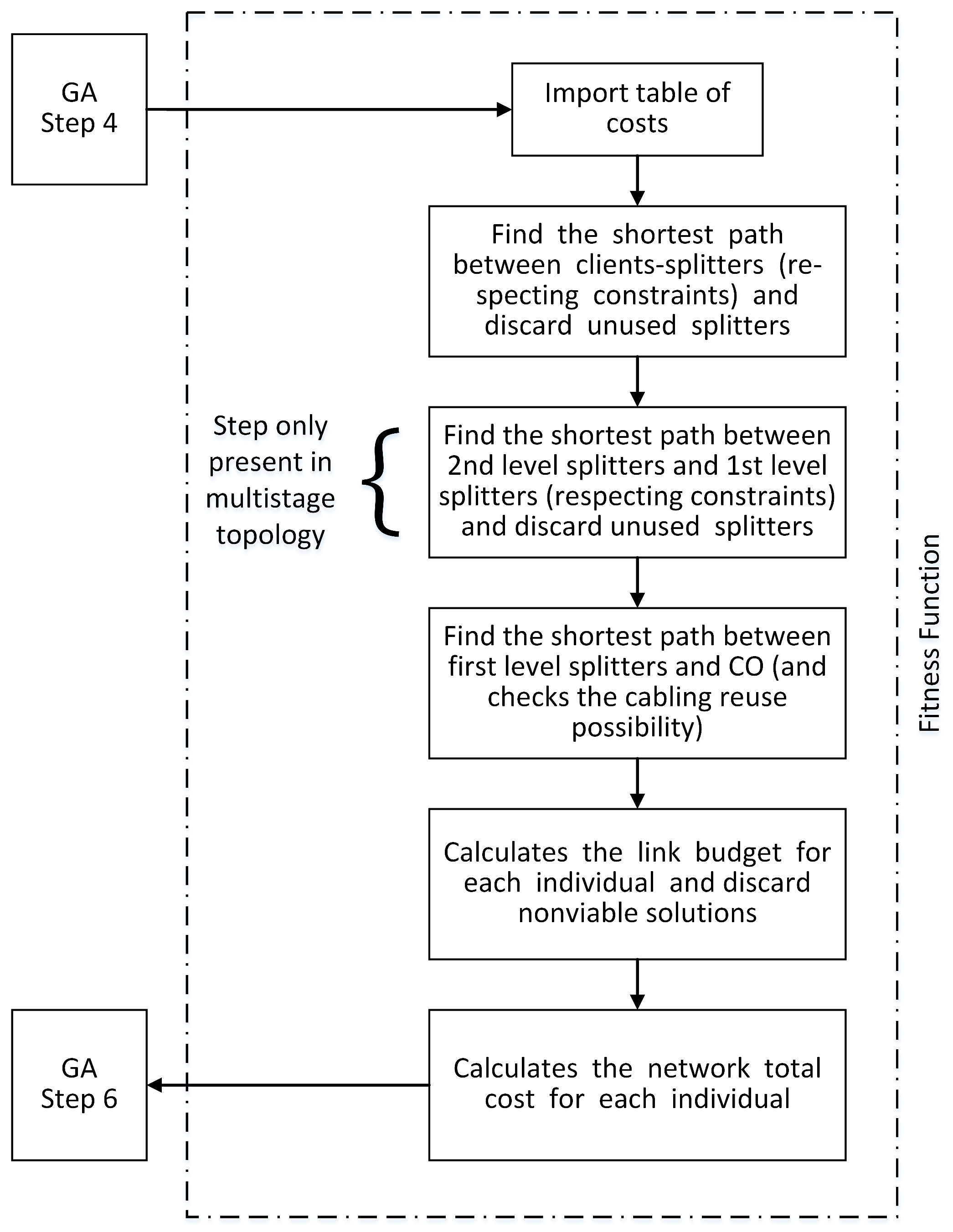
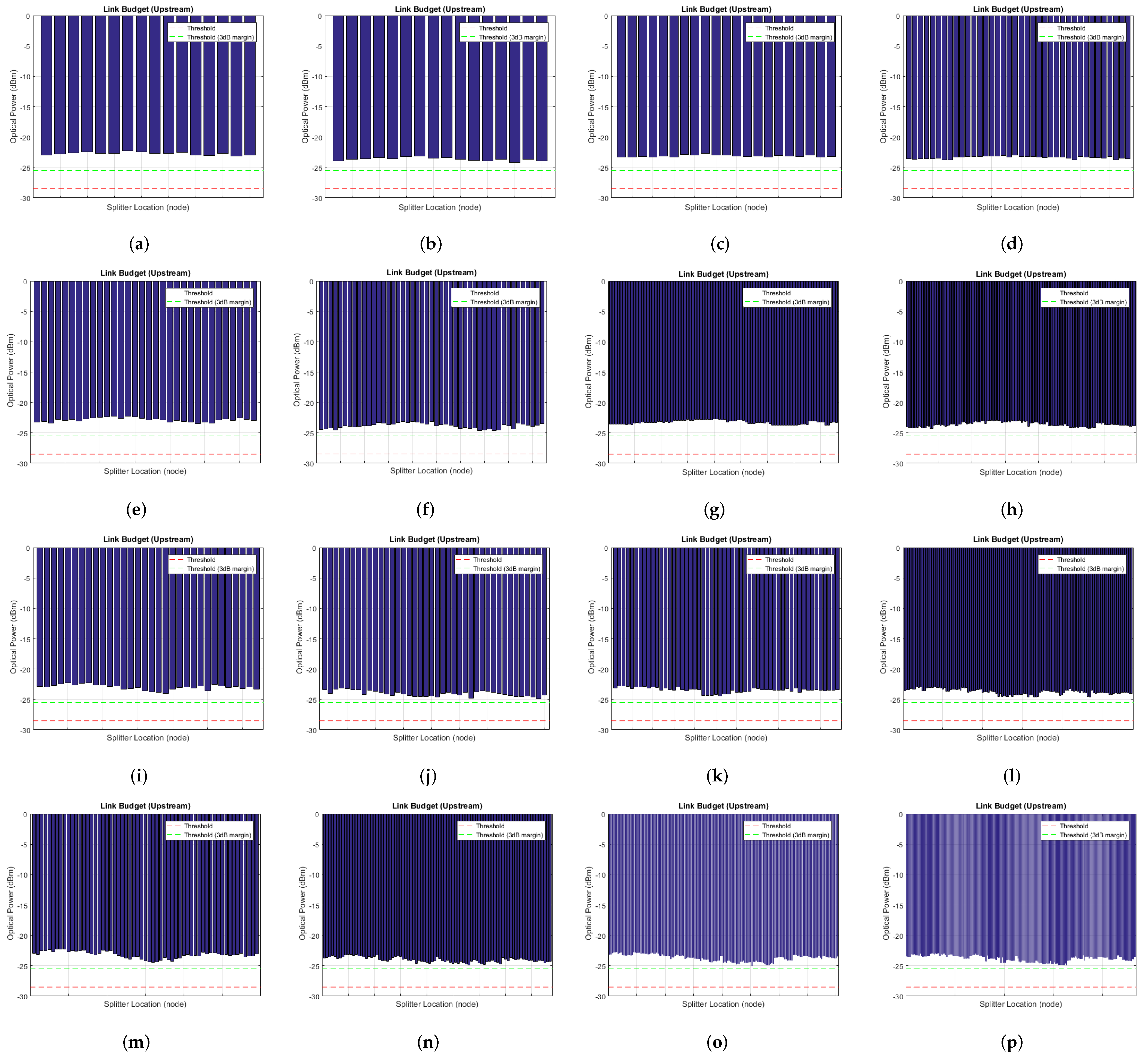
• (5) Calculate the individual cost (fitness function): With the individuals generated in the previous step (step 4), and the obtained information from the map, the network is set up for each individual and the total cost (for each individual) is calculated. The network total cost (in R$) is represented by the sum of all materials and services involved in the network deployment. Figure 7 shows the flowchart and the following steps describe in details the fitness function steps:
  ($5.1$) Import table of costs: First of all, the table of costs for PON deployment containing materials and installing service costs is imported. These costs were reported by a real ISP of Salvador city, Brazil;
  ($5.2$) Find the shortest path between subscribers–splitters (respecting constraints) and discard unused splitters: Using matrix operations, the algorithm finds the shortest path between all subscribers and splitters (respecting the following constraints: (1) the last mile connection will always use a drop cable and must respect the maximum limit of 400 m; (2) the number of subscribers served by an optical splitter cannot be greater than the number of available ports; (3) every subscriber must be connected to an optical splitter). Splitters that do not have assigned subscribers are discarded (gene value in the specific position of the matrix is set to 0). Individuals who do not meet the restrictions have their costs defined as infinite and, consequently, are discarded in the next generations;
  ($5.3$) Find the shortest path between 2nd level splitters and 1st level splitters (respecting constraints) and discard unused splitters: Similarly to step ($5.2$), using matrix operations, the algorithm calculates the shortest path between all 2nd and 1st level splitters (if a multiple stage is adopted). Connections must respect the available ports of first level splitters. Empty splitters are discarded;
  ($5.4$) Find the shortest path between 1st level splitters and CO (and check the cabling reuse possibility): Again, using matrix operations, the algorithm calculates the shortest path between all 1st level splitters and CO. Based on the found minimum distances, the algorithm checks the possibility of creating a shared feeder cable route among 1st level splitters;
  ($5.5$) Calculate the link budget for each individual and discard non-viable solutions: In this step, the individual optical power budget is also calculated. For the calculus of optical attenuation, typical attenuation values defined on the ITU-T G.671 recommendation [40] were used, which characterizes optical components. To complement and to increase the accuracy of the calculation, we also adopted a vendor (Furukawa) real typical values of attenuation for passive (

  Table 3. Typical losses adopted for network passive elements.

  Component	Typical Loss	Reference or Part-Number
  Drop Cable (02F)	0.37 dB/km (for 1310 nm)	17042026
  Distribution Cable (12F)		17045113
  Feeder Cable (48F)		17040049
  Optical Splitter 1 × 2	3.7 dB	35500123
  Optical Splitter 1 × 4	7.1 dB	35505000
  Optical Splitter 1 × 8	10.5 dB	35505001
  Optical Splitter 1 × 16	13.7 dB	35505002
  Optical Splitter 1 × 32	17.1 dB	35505003
  Optical Splitter 1 × 64	20.5 dB	35505047
  Aligned fusion splice	0.08 dB	ITU-T G.671
  Mechanical splice	0.15 dB	ITU-T G.671
  Optical Connector	0.3 dB	ITU-T G.671

  ) and active network elements (

  Table 4. Typical losses adopted for network active elements.

  Component	Average Launch Power	Receiver Optical Overload	Receiver Sensitivity	Reference Part-Number
  OLT (SFP CLASSE B+)	1.5 to 5 dBm	−8 dBm	−28 dBm	35510197
  ONT (ONT FK-G421W)	0.5 to 5 dBm	−8 dBm	−27 dBm	35510133

  ). It is worth mentioning that, for optical link budget calculation, the lowest value of launched power was considered (worst case).
  In the proposed algorithm, the optical attenuation was calculated only for the 1310 nm wavelength (used for GPON upstream). This is due to the greater optical losses in this wavelength and, therefore, it can define the condition of the network functioning properly. The received power and total attenuation can be calculated for each optical link by

  $$P_r=P_{tx}-\sum P_{at},$$

  (5)

  and

  $$\sum P_{at}=\sum {\alpha }_c+\sum {\alpha }_s+\sum {\alpha }_{sp}+\sum \left({\alpha }_{f,\lambda }L\right),$$

  (6)

  in which $P_r$ represents the received power (in dBm), $P_{tx}$ the transmitted power (in dBm), $\sum P_{at}$ the sum of link attenuation (in dB), $\sum {\alpha }_c$ the total loss of each optical connector (in dB), $\sum {\alpha }_s$ the total loss of each splice (in dB), $\sum {\alpha }_{sp}$ the total loss of optical splitters (in dB), $\sum ({\alpha }_{f,\lambda }\times L)$ the fiber loss (in dB/km) for the wavelength $\lambda$ and L the optical link length (in km). In this paper, we only considered power budget in our proposal. Crosstalk analysis between different wavelength channels and the impact of the transmission impairments (chromatic dispersion, laser phase noise, fiber nonlinearity and limitations due to Kerr nonlinearity) are part of proposals for future works;
  ($5.6$) Calculate the network total cost for each individual: using the imported cost table, the shortest distances already stored and knowing the positions of all optical splitters, the network cost (in R$) is calculated (for each individual).
• (6) Select the most fit individuals: In this step, individuals are organized in ascending order according to each value of total deployment cost obtained by using the fitness function (step 5). Part of the most fit individuals are copied and maintained (to guarantee not worse solutions). Then, the most fit individuals (best solutions) are selected and participate in the crossover and mutation procedures (step 7). The rest of the individuals are discarded (do not participate in next generations).
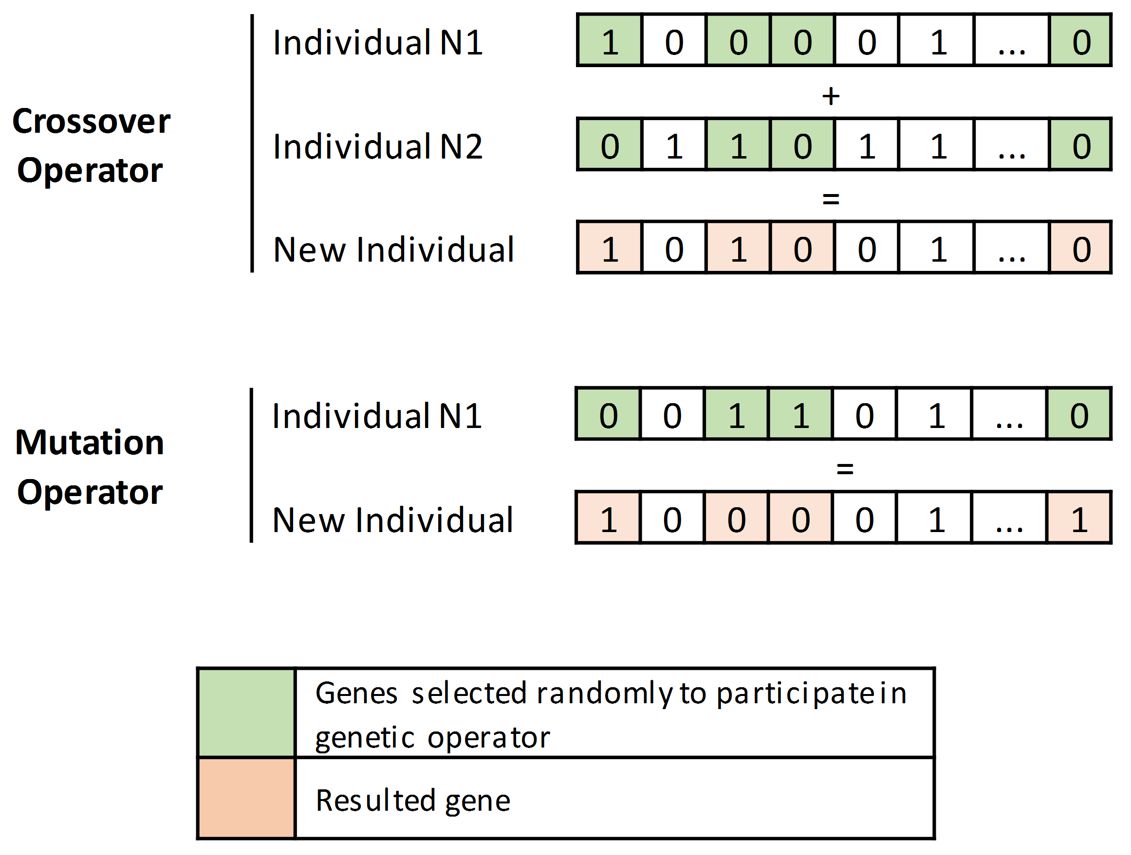
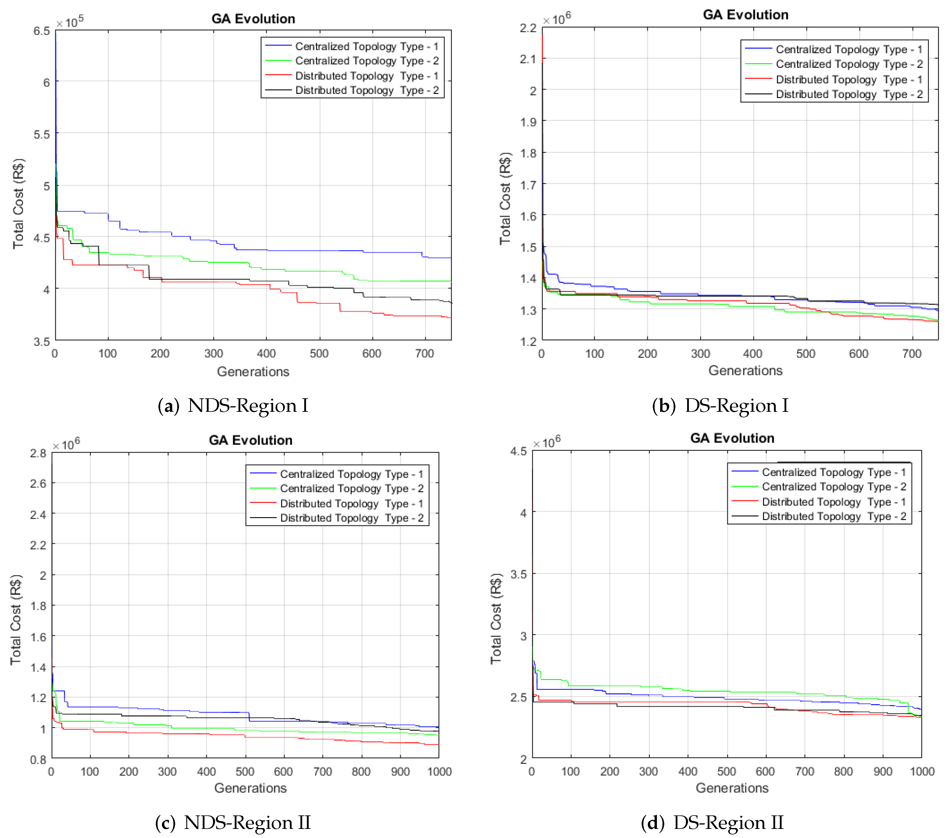
• (7) Crossover and mutation procedures: The genetic operators are applied to the selected individuals in the previous step (step 6). The crossover function randomly combines characteristics (genes) of two individuals (among those selected). In the crossover operation, genes not drawn will inherit the values of the first selected individual. The mutation function arbitrarily alters one or more characteristics (genes) of the selected individual. Figure 8 shows a graphical example of the crossover and mutation genetic operators applied to hypothetical individuals.
  For better results, an index-to-check and method to monitor the remaining number of generations have been developed. In this way, as the generations advance, the system reduces the probability of too many changes in the genes of the selected individuals (through genetic operators). This adjustment allows a greater chance of fine-tuning when individuals have an advanced generation index. It is worth mentioning that all probability parameters were set empirically.
• (8) New population: in this step, the new population is stored and is formed by: a part of the most fit individuals maintained in step (step 6)—for keeping the most fit individuals in case of worsening solutions—and new individuals emerged from the genetic operators such as crossover and mutation. With the new population, the algorithm performs G interactions (repeating the previous steps 1 to 7) until reach the predefined value for generations. When this value reaches $G_{\mathrm{Max}}$, the algorithm recalculates the network cost for the last stored population and the best individual is considered as the final solution to the proposed problem.

5. Simulation Setup

In our simulation scenarios, we considered two Brazilian regions and we called them Region I and Region II. For both regions, we suppose an ISP willing to deploy a new GPON network. The GPON technology operation is outlined in the ITU-T G.984.x standards series and its main characteristics are described in

Table 5. GPON characteristics and adopted values.

	ITU-T G.984 (GPON) [12]	ADOPTED GPON SYSTEM
Downstream Rate	2.5 Gbps	2.5 Gbps
Upstream Rate	1.25 or 2.5 Gbps	1.25 Gbps
Downstream Wavelength	1490 nm	1490 nm
Upstream Wavelength	1310 nm	1310 nm
Broadcast RF Video Wavelength	1510 nm	-
Physical Reach	10 or 20 km	20 km
Split ratio	1:32, 1:64, (1:128 planned)	1:64

(together with values adopted in all simulations carried on in this work).

The first region is the central part of Pituba neighborhood (Region I). This region is located in the south of Salvador city, Bahia, Brazil. This region has approximately $1.85$ km${}^2$ of area and, after the importation process, is represented by a graph of 314 nodes. This choice is due to the medium–large size of the neighborhood. The second region is significantly larger and has a larger number of nodes. It is the central part of Camaçari, another city of Bahia state in Brazil (Region II). This second region has approximately $5.7$ km${}^2$ of area and, after the importation process, is represented by a graph of 714 nodes. This choice is mainly due to the large size of the resultant graph and also because this region represents a large-sized non-capital city in Brazil.

Both regions (Region I and Region II) were tested in two different scenarios, called non-dense and dense scenario (NDS and DS, respectively). The first one (NDS) consists of a scenario in which subscribers are distributed in a dispersed manner in the region of interest. The second scenario (DS) has a considerably higher number of subscribers distributed in a very close way to each other. Figure 5 shows the network initial state for non-dense and dense simulation scenarios, considering a network with 314 nodes (Region I) and 714 nodes (Region II). It is worth mentioning that the subscribers’ distribution in the graph was carried out in a random manner. For the non-dense scenario, there is a predominance of nodes with two subscribers (green nodes). For the dense scenario, there is a higher incidence of nodes with seven subcribers (red nodes).

All the simulations in this paper were done under Intel^® Core i5 $1.8$ GHz processor, with 8 GB of RAM and Windows 8^®. The PONs planning optimization was based on a GA technique (as described in detail in Section 4.3) and developed in Matlab^® software.

Table 6. Network initial characteristics for Region I and Region II (with non-dense and dense scenarios).

Network Characteristics	Region I		Region II
	Values (NDS)	Values (DS)	Values (NDS)	Values (DS)
Initial population (individuals)	125	125	125	125
Number of generations (iterations)	750	750	1000	1000
Selection percentage (%)	40	40	40	40
Reserve for future subscribers (%)	$12.50$	$12.50$	$12.50$	$12.50$
Number of nodes	314	314	714	714
Total number of attended subscribers	164	820	436	1544
Nodes with 2 subscribers (green color)	52	11	151	6
Nodes with 4 subscribers (yellow color)	8	35	21	19
Nodes with 7 subscribers (red color)	4	94	6	208
Map area (km${}^2$)	$1.85$	$1.85$	$5.7$	$5.7$
subscribers/km${}^2$	88	443	76	$270.87$

describes the network initial characteristics for Region I and Region II (with non-dense and dense scenarios).

6. Results

The results are discussed in terms of genetic algorithm solutions and evolution, network optical power link budget and a comparison of the main information generated by the genetic algorithm. For centralized topologies, the green line represents the route of the feeder optical cable and the red diamond represents access splitters. For distributed topologies, the orange line represents the distribution cable. In addition, the red diamond represents first level splitters (distribution) and the black star represents second level splitters (access).

Figure 5a,b (Figure 5c,d) show, respectively, the network initial state for non-dense and dense scenario, considering Region I with 314 nodes (and Region II with 714 nodes). This initial state will be used as an algorithm’s input to find a solution for each one of the four considered topologies in this paper (as can be seen in details in Section 3).

For non-dense scenario, an index of approximately 88 subscribers was obtained per km${}^2$ for Region I (76 subscribers was obtained per km${}^2$ for Region II). The number of generations was set, empirically, at 750. It was observed that, using higher values, there are no major changes in the final network total cost. For dense scenario, the incidence of nodes with seven subscribers in the initial state was predominant. An index of approximately 443 subscribers was obtained per km${}^2$ for Region I ($270.87$ subscribers was obtained per km${}^2$ for Region II). Again, it should be noted that subscribers were randomly distributed in the graph.

Figure 9a–d (Figure 9i–l) shows the GA solutions for non-dense and Figure 9e–h (Figure 9m–p) for dense scenario in Region I (Region II), considering: (a) CTT1; (b) CTT2; (c) DTT1 and (d) DTT2. In CTT2, first level splitters are not represented (because they are placed at CO). Although considered in total cost, the last mile of cable is not represented in the figure to avoid too much data exhibition.

Figure 10a,b and Figure 10c,d show, respectively, the GA evolution for each topology for the non-dense and dense scenarios, considering Region I Region II. As can be observed, there is a substantial reduction of the total network cost between the initial populations and the last ones. In addition, we can observe that negligible reductions are achieved if more generations are used. The stop criteria of 750 generations for Region I NDS and 1000 generations for Region I DS was set empirically.

Figure 11a–d (Figure 11i–l) show the network link budget for non-dense and Figure 11f–h (Figure 11m–p) for dense scenario in Region I (Region II), considering: (a) CTT1; (b) CTT2; (c) DTT1 and (d) DTT2. Each bar represents the received optical power (in the upstream transmission) of each link between OLT and network proposed access splitters. We chose not to consider each ONT here to avoid too much data exhibition. However, in each link calculation, it was considered the longest drop cable connected to each access splitter (furthest subscriber—worst case). In addition, x axis represents, sequentially, the position (node) of each access splitter on the graph. Due to the high number of access splitters and the reduced scale, we chose not to show this information. The red and the green dotted line show, respectively, the receiver sensitivity (threshold) in upstream transmission and the receiver sensitivity considering an additional safety margin of 3 dB. This safety margin is used to allow for unexpected losses and ensure performance criteria are met.

Table 7. Comparison of the main information generated by the genetic algorithm for the four possible topologies, considering non-dense and dense scenario, for Region I.

Item	Region I (NDS)				Region I (DS)
	CTT1	CTT2	DTT1	DTT2	CTT1	CTT2	DTT1	DTT2
Execution time (min)	25.14	31.52	27.13	33.62	19.21	35.12	27.14	29.02
2F cable (drop cable) (km)	26.98	26.46	21.65	12.78	78.09	60.99	48.67	40.35
12F cable (distribution cable) (km)	-	-	6.78	11.09	-	-	12.22	22.65
48F cable (feeder cable) (km)	6.58	6.64	2.05	2.99	9.83	11.57	7.31	7.16
Total used optical cables (km)	33.56	33.10	30.49	26.86	87.92	72.56	68.19	70.16
Total used 1st level splitters (unit)	16	8	8	8	32	24	28	24
Total used 2nd level splitters (unit)	-	16	21	38	-	47	86	138
Total used FOSC (unit)	16	16	7	8	32	47	22	22
Total used PON ports (unit)	16	8	8	8	32	24	28	24
Network total cost (R$)	430,122.38	406,639.48	371,720.02	385,718.94	1,294,399.87	1,261,623.09	1,259,180.97	1,312,597,11
Increased cost (%)	13.58	8.59	-	3.63	2.72	0.19	-	4.06

and

Table 8. Comparison of the main information generated by the genetic algorithm for the four possible topologies, considering non-dense and dense scenario, for Region II.

Item	Region II (NDS)				Region II (DS)
	CTT1	CTT2	DTT1	DTT2	CTT1	CTT2	DTT1	DTT2
Execution time (min)	63.35	61.08	64.17	63.55	76.58	70.05	66.73	72.27
2F cable (drop cable) (km)	79.93	63.83	54.15	27.82	141.20	114.68	84.78	73.03
12F cable (distribution cable) (km)	-	-	19.66	29.07	-	-	23.32	42.17
48F cable (feeder cable) (km)	13.95	16.16	6.69	11.09	17.73	19.64	14.16	13.01
Total used optical cables (km)	93.88	79.99	80.50	67.98	158.93	134.31	122.26	128.21
Total used 1st level splitters (unit)	32	20	16	24	59	44	51	39
Total used 2nd level splitters (unit)	-	40	54	115	-	87	161	233
Total used FOSC (unit)	32	40	13	24	59	87	43	36
Total used PON ports (unit)	32	20	16	24	59	44	51	39
Network total cost (R$)	1,005,588.35	945,542.69	889,545.10	971,691.88	2,394,071.30	2,237,337.33	2,329,664.76	2,343,312.70
Increased cost (%)	11.54	5.92	-	8.45	2.69	0.32	-	0.66

describe a comparison of the main information generated by the genetic algorithm for the four possible topologies, considering the non-dense and dense scenarios, for Region I Region II, respectively. It is worth mentioning that, in the maps plotted by the GA, the identification number of each node was hidden to improve the visualization of the graphical results (due to the reduced scale).

7. Conclusions

We proposed a new approach based on GA for optimization of PON planning. Tests on a large-size scenario proved the potential of the tool. In addition, the obtained results for the proposed scenarios show that the adopted topology in each project has a direct influence on the total cost of the network deployment. The distributed topology type 1 (DTT1) presented the lowest implantation cost, followed closely by the distributed topology type 2 (DTT2). This fact is justified due to the greater amount of splitters (of access) used in the network, reducing the amount of last mile cables (which represents a considerable part of the total cost of implementation). However, splitters with large capacity have a high cost and need a large concentration of subscribers in order to dilute their cost among them. Therefore, the trend is that, in scenarios with few subscribers, access splitters with smaller capacities have lower related costs, which makes distributed solutions more adapted to these situations. It is then noted that there is a clear relationship between subscribers location, splitters, PON ports and optical cables. Regarding the optical power link budget, all the solutions found by GA are above the threshold, which means an adequate operation of the proposed GPON system.

References

1. Butt, R.A.; Faheem, M.; Ashraf, M.W. Efficient upstream bandwidth utilization with minimum bandwidth waste for time and wavelength division passive optical network. Opt. Quant. Electron. 2020, 52, 14. [Google Scholar] [CrossRef]
2. Mat Sharif, K.A.; Ngah, N.A.; Ahmad, A.; Khairi, K.; Manaf, Z.A.; Tarsono, D. Demonstration of xgs-pon and gpon co-existing in the same passive optical network. In Proceedings of the IEEE 7th International Conference on Photonics (ICP), Langkawi, Malaysia, 9–11 April 2018. [Google Scholar] [CrossRef]
3. Liu, X.; Effenberger, F. Emerging Optical Access Network Technologies for 5G Wireless [Invited]. J. Opt. Commun. Netw. 2016, 8, B70–B79. [Google Scholar] [CrossRef]
4. Cisco Annual Internet Report (2018–2023). Available online: https://www.cisco.com/c/en/us/solutions/collateral/executive-perspectives/annual-internet-report/white-paper-c11-741490.html (accessed on 26 February 2022).
5. Household Broadband Guide. Available online: https://www.fcc.gov/consumers/guides/household-broadband-guide (accessed on 26 February 2022).
6. Fourie, H.; Bijl, P.W. Race to the top: Does competition in the DSL market matter for fibre penetration? Telecomm Policy 2018, 42, 778–793. [Google Scholar] [CrossRef]
7. Prat, J. Next-Generation FTTH Passive Optical Networks; Springer: Dordrecht, The Netherlands, 2008. [Google Scholar] [CrossRef]
8. Muciaccia, T.; Gargano, F.; Passaro, V.M.N. Passive Optical Access Networks: State of the Art and Future Evolution. Photonics 2014, 1, 323–346. [Google Scholar] [CrossRef]
9. Fixed Broadband Access in Brazil. Available online: https://informacoes.anatel.gov.br/paineis/acessos/banda-larga-fixa (accessed on 26 February 2022).
10. Chen, J.; Wosinska, L.; Mas Machuca, C.; Jaeger, M. Cost vs. reliability performance study of fiber access network architectures. IEEE Commun. Mag. 2010, 48, 56–65. [Google Scholar] [CrossRef]
11. Lam, C.F. Passive Optical Networks: Principles and Practice; Academic Press: Burlington, VT, USA, 2007; pp. 1–324. [Google Scholar]
12. Recommendation G.984.1: Gigabit-Capable Passive Optical Networks (GPON): General Characteristics. Available online: https://www.itu.int/rec/T-REC-G.984.1 (accessed on 26 February 2022).
13. Recommendation G.9807.1: 10-Gigabit-Capable Symmetric Passive Optical Network (XGS-PON). Available online: https://www.itu.int/rec/T-REC-G.9807.1/en (accessed on 26 February 2022).
14. Recommendation G.9804.1: Higher Speed Passive Optical Networks. Available online: https://www.itu.int/rec/T-REC-G.9804.1-201911-I/en (accessed on 26 February 2022).
15. Poon, K.F.; Mortimore, D.B.; Mellis, J. Designing optimal FTTH and PON networks using new automatic methods. In Proceedings of the International Conference on Access Technologies, Cambridge, UK, 21–22 June 2006; pp. 45–48. [Google Scholar] [CrossRef]
16. Arokkiam, J.A.; Alvarez, P.; Wu, X.; Brown, K.N.; Sreenan, C.J.; Ruffini, M.; Marchetti, N.; Doyle, L.; Payne, D. Design, implementation, and evaluation of an xg-pon module for the ns-3 network simulator. Simulation 2017, 93, 409–426. [Google Scholar] [CrossRef]
17. Kokangul, A.; Ari, A. Optimization of passive optical network planning. Appl. Math. Modell. 2011, 35, 3345–3354. [Google Scholar] [CrossRef]
18. Chu, A.; Poon, K.F.; Ouali, A. Using ant colony optimization to design GPON-FTTH networks with aggregating equipment. In Proceedings of the Symposium on Computational Intelligence for Communication Systems and Networks (CIComms), Singapore, 16–19 April 2013; pp. 10–17. [Google Scholar] [CrossRef]
19. Ouali, A.; Poon, K.F.; Lee, B.; Romaithi, K.A. Towards achieving practical GPON FTTH designs. In Proceedings of the International Workshop on Computer Aided Modelling and Design of Communication Links and Networks (CAMAD), Guildford, UK, 7–9 September 2015; pp. 108–113. [Google Scholar] [CrossRef]
20. Pehnelt, T.; Lafata, P. Optimizing of passive optical network deployment using algorithm with metrics. Adv. Electr. Electron. Eng. 2018, 15, 866–876. [Google Scholar] [CrossRef]
21. Villalba, T.V.Y.; Rossi, S.M.; Mokarzel, M.P.; Salvador, M.R.; Neto, H.M.A.; Cesar, A.C.; Romero, M.A.; Rocha, M.D.L. Design of passive optical networks using genetic algorithm. In Proceedings of the SBMO/IEEE MTT-S International Microwave and Optoelectronics Conference (IMOC), Belem, Brazil, 3–6 November 2009; pp. 682–688. [Google Scholar] [CrossRef]
22. Eira, A.; Pedro, J.; Pires, J. Optimized design of multistage passive optical networks. J. Opt. Commun. Netw. 2012, 4, 402–411. [Google Scholar] [CrossRef]
23. Yang, H.; Zhang, J.; Ji, Y.; Lee, Y. C-RoFN: Multi-stratum resources optimization for cloud-based radio over optical fiber networks. IEEE Commun. Mag. 2016, 54, 118–125. [Google Scholar] [CrossRef]
24. Yang, H.; Yuan, J.; Li, C.; Zhao, G.; Sun, Z.; Yao, Q.; Bao, B.; Vasilakos, A.V.; Zhang, J. BrainIoT: Brain-like productive services provisioning with federated learning in industrial IoT. IEEE Internet Things J. 2021, 9, 2014–2024. [Google Scholar] [CrossRef]
25. Yang, H.; Zhang, J.; Zhao, Y.; Han, J.; Lin, Y.; Lee, Y. SUDOI: Software defined networking for ubiquitous data center optical interconnection. IEEE Commun. Mag. 2016, 54, 86–95. [Google Scholar] [CrossRef]
26. Europe, F.C. FTTH Handbook, 8th ed.; FTTH Council Europe: Brussel, Belgium, 2018; Available online: https://www.c3comunicaciones.es/Documentacion/FTTH%20Handbook_2017_V8_FINAL.pdf (accessed on 26 February 2022).
27. Arévalo, G.V.; Hincapié, R.C.; Gaudino, R. Optimization of multiple PON deployment costs and comparison between GPON, XGPON, NGPON2 and UDWDM PON. Opt. Switch. Net. 2017, 25, 80–90. [Google Scholar] [CrossRef] [Green Version]
28. FTTH Architecture White Paper Series. Available online: https://www.commscope.com/globalassets/digizuite/2597-ftth-architectures-wp-110964-en.pdf?r=1 (accessed on 26 February 2022).
29. Cavalcante, M.A.; Pereira, H.A.; Chaves, D.A.R.; Almeida, R.C. An auxiliary-graph-based methodology for regenerator assignment problem optimization in translucent elastic optical networks. Opt. Fiber Technol. 2019, 53, 102008. [Google Scholar] [CrossRef]
30. Holland, J.H. Genetic Algorithms. Sci. Am. 1992, 267, 66–73. [Google Scholar] [CrossRef]
31. Srinivas, M.; Patnaik, L.M. Genetic algorithms: A survey. IEEE Comput. 1994, 27, 17–26. [Google Scholar] [CrossRef]
32. Sivanandam, S.N.; Deepa, S.N. Genetic Algorithm Optimization Problems; Introduction to Genetic Algorithms; Springer: Berlin/Heidelberg, Germany, 2008. [Google Scholar] [CrossRef]
33. Moza, M.; Kumar, S. Routing in networks using genetic algorithm. Int. J. Commun. Net. Dist. Syst. 2018, 20, 291–311. [Google Scholar] [CrossRef]
34. Moza, M.; Kumar, S. Network routing protocol using genetic algorithms. Int. J. Electr. Comput. Sci. 2010, 10, 36–40. [Google Scholar]
35. Leung, Y.; Li, G.; Xu, Z.B. A genetic algorithm for the multiple destination routing problems. IEEE Trans. Evol. Comput. 1998, 2, 150–161. [Google Scholar] [CrossRef]
36. Sun, B.; Li, L. A QoS multicast routing optimization algorithm based on genetic algorithm. J. Commun. Netw. 2006, 8, 116–122. [Google Scholar] [CrossRef]
37. Beckmann, D.; Killat, U. Routing and wavelength assignment in optical networks using genetic algorithms. Eur. Trans. Telecom. 1999, 10, 537–544. [Google Scholar] [CrossRef]
38. Rani, K.S.K.; Deepa, S.N. Hybrid evolutionary computing algorithms and statistical methods based optimal fragmentation in smart cloud networks. Cluster Comput 2019, 22, 241–254. [Google Scholar] [CrossRef]
39. Floyd, R.W. Algorithm 97: Shortest path. Comm. ACM 1962, 5, 318–328. [Google Scholar] [CrossRef]
40. G.671: Transmission Characteristics of Optical Components and Subsystems. Available online: https://www.itu.int/rec/T-REC-G.671/en (accessed on 26 February 2022).
Figure 1. Physical topology diagram for: (a) CTT1, (b) CTT2, (c) DTT1 and (d) DTT2.
Photonics 09 00278 g001
Figure 2. A simple, non-oriented graph, in which V represents vertices (or nodes) and E represents edges (or links).
Photonics 09 00278 g002
Figure 3. Flowchart of our proposed genetic algorithm for optimization of PONs planning.
Photonics 09 00278 g003
Figure 4. Graphical example of importing georeferenced data to Matlab®, considering: (a) interest (Costa Azul neighborhood) with overlapping graph; (b) example of a region of interest to be imported into Matlab®; and (c) network graph, containing 108 nodes, imported into Matlab®.
Photonics 09 00278 g004
Figure 5. Network initial state for non-dense and dense simulation scenarios, considering network topologies with 314 nodes (Region I) and 714 nodes (Region II). (a) NDS-Region I, (b) DS-Region I, (c) NDS-Region II, (d) DS-Region II.
Photonics 09 00278 g005
Figure 6. Graphical example of the first individuals of the initial population matrices (with two optical splitter levels) presented in Equations (3) and (4). Each pair of individuals in the matrices will represent a different solution for the problem.
Photonics 09 00278 g006
Figure 7. Flowchart of the fitness function steps.
Photonics 09 00278 g007
Figure 8. Graphical example of the crossover and mutation genetic operators applied to hypothetical individuals.
Photonics 09 00278 g008
Figure 9. GA solutions for non-dense and dense scenario (with 314 and 714 nodes), considering four possible topologies (CTT1, CTT2, DTT1 and DTT2). (a) NDS-Region I-CTT1, (b) NDS-Region I-CTT2, (c) NDS-Region I-DTT1, (d) NDS-Region I-DTT2, (e) DS-Region I-CTT1, (f) DS-Region I-CTT2, (g) DS-Region I-DTT1, (h) DS-Region I-DTT2, (i) NDS-Region II-CTT1, (j) NDS-Region II-CTT2, (k) NDS-Region II-DTT1, (l) NDS-Region II-DTT2, (m) DS-Region II-CTT1, (n) DS-Region II-CTT2, (o) DS-Region II-DTT1, (p) DS-Region II-DTT2.
Photonics 09 00278 g009
Figure 10. GA solutions for non-dense and dense scenario (with 314 and 714 nodes), considering: (a) CTT1; (b) CTT2; (c) DTT1 and (d) DTT2.
Photonics 09 00278 g010
Figure 11. Network link budget for non-dense and dense scenario (with 314 and 714 nodes), considering four possible topologies (CTT1, CTT2, DTT1 and DTT2). (a) NDS-Region I-CTT1, (b) NDS-Region I-CTT2, (c) NDS-Region I-DTT1, (d) NDS-Region I-DTT2, (e) DS-Region I-CTT1, (f) DS-Region I-CTT2, (g) DS-Region I-DTT1, (h) DS-Region I-DTT2, (i) NDS-Region II-CTT1, (j) NDS-Region II-CTT2, (k) NDS-Region II-DTT1, (l) NDS-Region II-DTT2, (m) DS-Region II-CTT1, (n) DS-Region II-CTT2, (o) DS-Region II-DTT1, (p) DS-Region II-DTT2.
Photonics 09 00278 g011