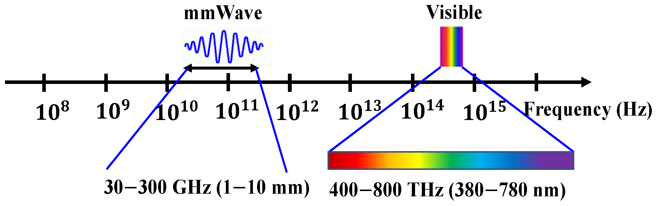
Propagation Characteristics Comparisons between mmWave and Visible Light Bands in the Conference Scenario


Abstract
:1. Introduction
1.1. Literature Review
1.2. Contributions of This Paper
- Channel characteristics comparisons between mmWave and VLC bands are performed based on the same conference scenario and parameter settings.
- A unique optical path loss (OPL) model dependent on the physical size of photodetectors (PDs) is first proposed for VLC based on the widely used floating-intercept (FI) model in mmWave. The size of PDs can be estimated to meet the required coverage range by using this model while designing systems.
- The large-scale fading characteristics and multipath-related characteristics, including root mean square (RMS) delay spread (DS), K-factor, and cluster characteristics, between mmWave and VLC bands are compared fairly based on the same scenario.
2. Scenarios and Setup
2.1. Measurement Scenario and Setup in mmWave Bands
- Setup one: Two omnidirectional biconical antennas (360° and 40° half power beam width (HPBW) in azimuth and elevation, respectively) were used at TX and RX sides to collect all multipath components (MPCs), and then 1000 channel impulse responses (CIRs) samples were measured in each position.
- Setup two: An omnidirectional biconical antenna was used at TX side while a directional horn antenna (10° and 11° HPBW in azimuth and elevation, respectively) was mounted in an electrical positioner at RX side. In these virtual measurements, the TX antenna was fixed and the RX antenna was rotated in steps of 5° in azimuth from 0° to 360°, and there were three different elevations, −10°, 0° and 10°. Channel characteristics in the spatial domain can be obtained through these virtual measurements. In each horn antenna pointing direction, we measured 1000 CIR samples.
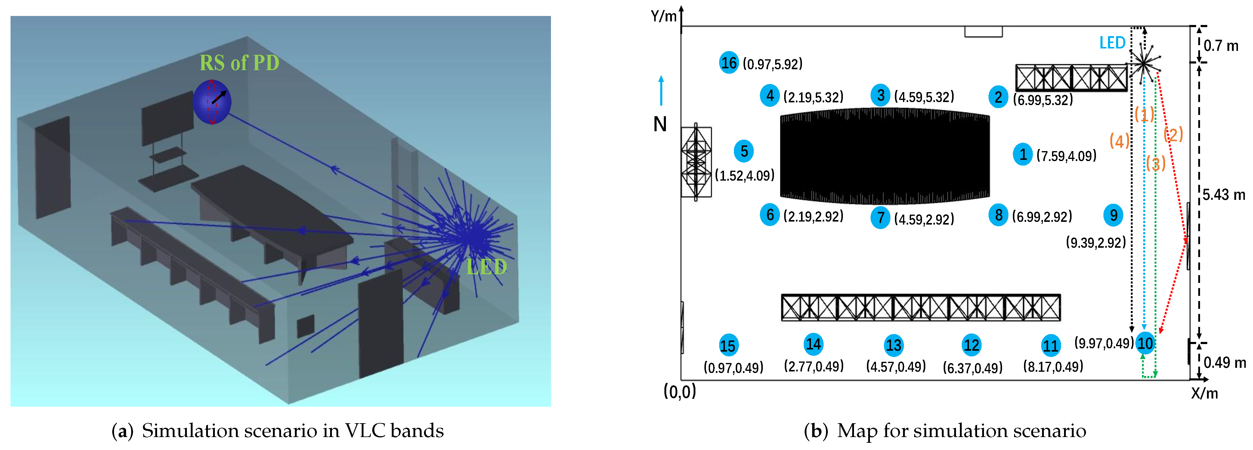
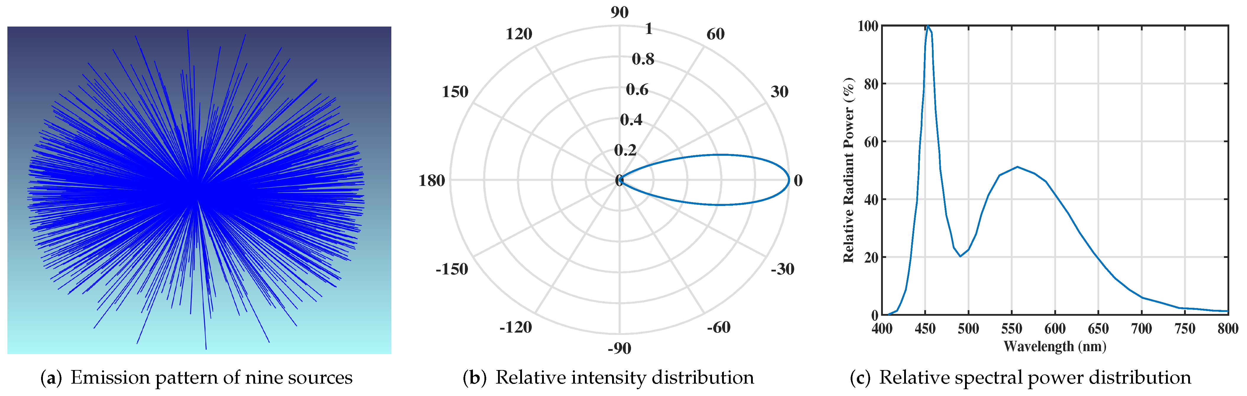
2.2. Simulation Scenario and Setup in VLC Bands
3. Channel Characteristics Comparisons
3.1. Channel Impulse Responses
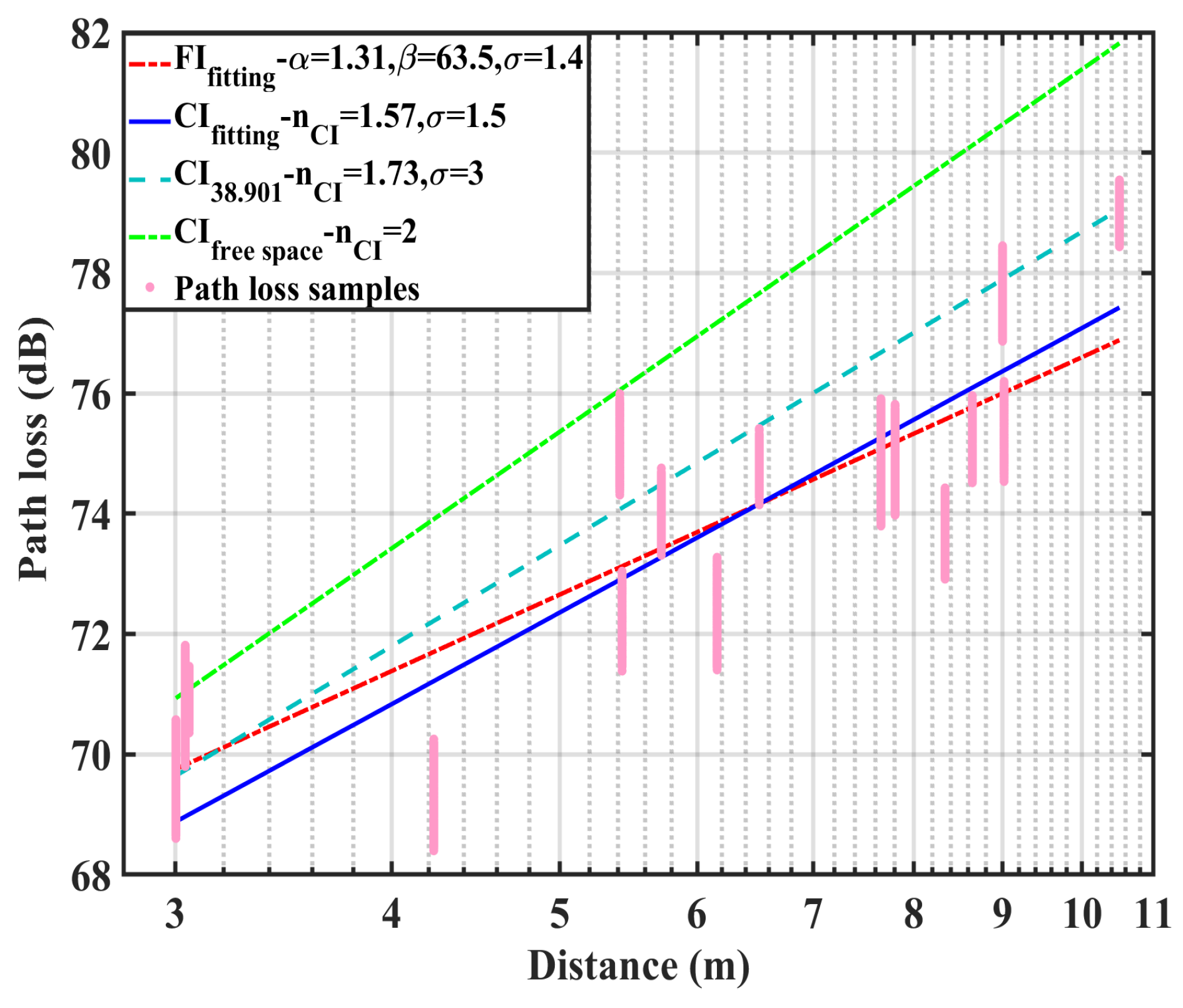
3.2. Path Loss
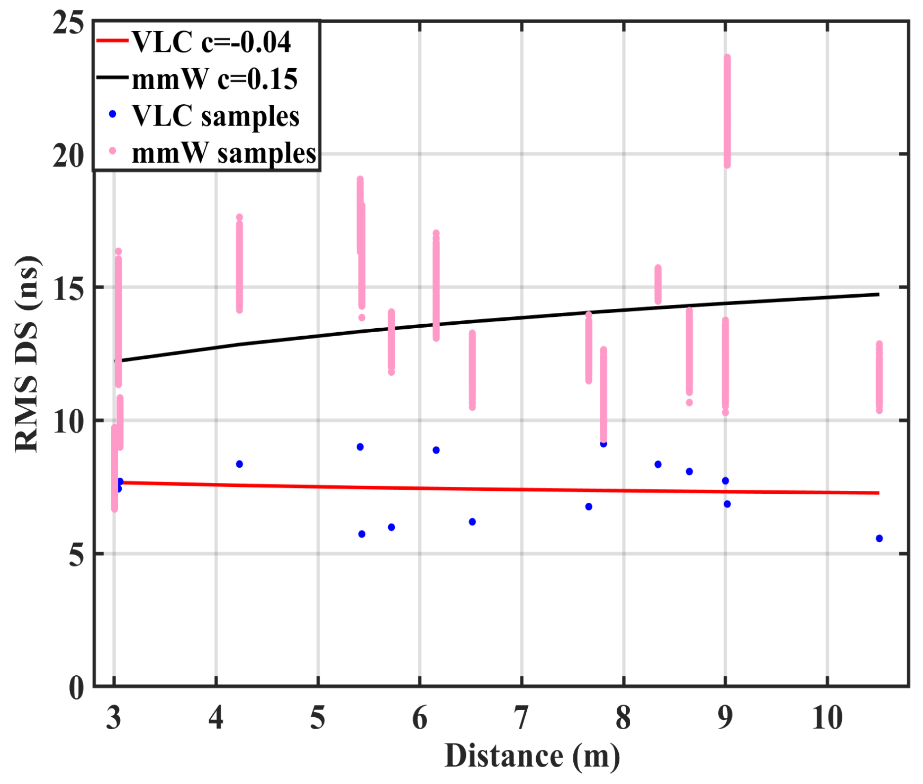
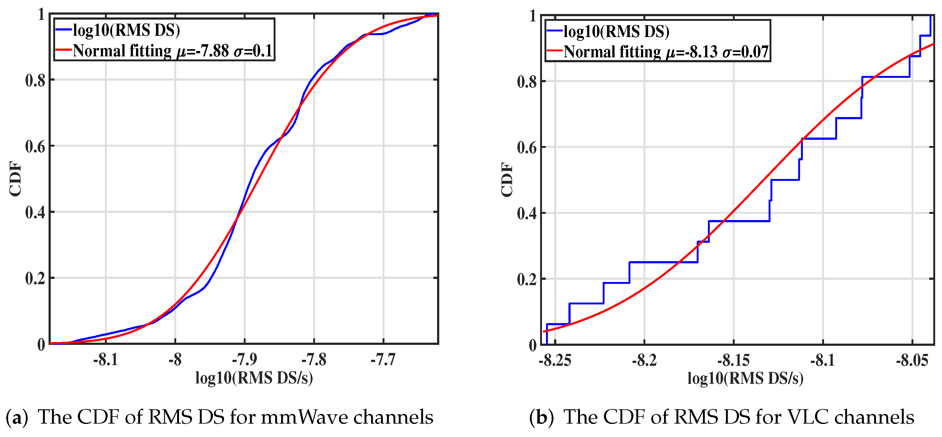
3.3. RMS DS
3.4. K-Factor
3.5. Cluster Characteristics
4. Conclusions and Future Work
Author Contributions
Funding
Institutional Review Board Statement
Informed Consent Statement
Data Availability Statement
Conflicts of Interest
References
- Sun, S.; Rappaport, T.S.; Shafi, M.; Tang, P.; Zhang, J.; Smith, P.J. Propagation models and performance evaluation for 5G millimeter-wave bands. IEEE Trans. Veh. Technol. 2018, 67, 8422–8439. [Google Scholar] [CrossRef]
- Tang, P.; Zhang, J.; Molisch, A.F.; Smith, P.J.; Shafi, M.; Tian, L. Estimation of the K-factor for temporal fading from single-snapshot wideband measurements. IEEE Trans. Veh. Technol. 2018, 68, 49–63. [Google Scholar] [CrossRef]
- Zhang, J.; Shafi, M.; Molisch, A.F.; Tufvesson, F.; Wu, S.; Kitao, K. Channel models and measurements for 5G. IEEE Commun. Mag. 2018, 56, 12–13. [Google Scholar] [CrossRef]
- Zhang, J.; Kang, K.; Huang, Y.; Shafi, M.; Molisch, A.F. Millimeter and THz wave for 5G and beyond. China Commun. 2019, 16. [Google Scholar]
- 3GPP. Study on Channel Model for Frequencies from 0.5 to 100 GHz. 3rd Generation Partnership Project, Technical Report TR 38.901 V16.1.0. 2019. Available online: https://portal.3gpp.org/desktopmodules/Specifications/SpecificationDetails.aspx?specificationId=3173 (accessed on 12 December 2021).
- Chi, N.; Zhou, Y.; Wei, Y.; Hu, F. Visible light communication in 6G: Advances, challenges, and prospects. IEEE Veh. Technol. Mag. 2020, 15, 93–102. [Google Scholar] [CrossRef]
- Zhang, J.H.; Tang, P.; Yu, L.; Jiang, T.; Tian, L. Channel measurements and models for 6G: Current status and future outlook. Front. Inf. Technol. Electron. Eng. 2020, 21, 39–61. [Google Scholar] [CrossRef]
- Chen, C.; Yang, H.; Du, P.; Zhong, W.D.; Alphones, A.; Yang, Y.; Deng, X. User-centric MIMO techniques for indoor visible light communication systems. IEEE Syst. J. 2020, 14, 3202–3213. [Google Scholar] [CrossRef]
- Gunawan, W.H.; Liu, Y.; Chow, C.W.; Chang, Y.H.; Yeh, C.H. High speed visible light communication using digital power domain multiplexing of orthogonal frequency division multiplexed (OFDM) signals. Photonics 2021, 8, 500. [Google Scholar] [CrossRef]
- Ji, R.; Wang, S.; Liu, Q.; Lu, W. High-speed visible light communications: Enabling technologies and state of the art. Appl. Sci. 2018, 8, 589. [Google Scholar] [CrossRef] [Green Version]
- Delgado-Rajo, F.; Melian-Segura, A.; Guerra, V.; Perez-Jimenez, R.; Sanchez-Rodriguez, D. Hybrid RF/VLC network architecture for the internet of things. Sensors 2020, 20, 478. [Google Scholar] [CrossRef] [Green Version]
- Qin, D.; Wang, Y.; Zhou, T. Performance analysis of hybrid radio frequency and free space optical communication networks with cooperative spectrum sharing. Photonics 2021, 8, 108. [Google Scholar] [CrossRef]
- Abuella, H.; Elamassie, M.; Uysal, M.; Xu, Z.; Serpedin, E.; Qaraqe, K.A.; Ekin, S. Hybrid RF/VLC systems: A comprehensive survey on network topologies, performance analyses, applications, and future directions. IEEE Access 2021, 9, 160402–160436. [Google Scholar] [CrossRef]
- Molisch, A.F. Wireless Communications, 2nd ed.; John Wiley & Sons: New York, NY, USA, 2012. [Google Scholar]
- Tavakkolnia, I.; Cheadle, D.; Bian, R.; Loh, T.H.; Haas, H. High speed millimeter-wave and visible light communication with off-the-shelf components. In Proceedings of the 2020 IEEE Globecom Workshops (GC Wkshps), Taiwan, China, 7–11 December 2020; pp. 1–6. [Google Scholar]
- Uyrus, A.; Turan, B.; Basar, E.; Coleri, S. Visible light and mmWave propagation channel comparison for vehicular communications. In Proceedings of the 2019 IEEE Vehicular Networking Conference (VNC), Los Angeles, CA, USA, 4–6 December 2019; pp. 1–7. [Google Scholar]
- Feng, L.; Yang, H.; Hu, R.Q.; Wang, J. MmWave and VLC-based indoor channel models in 5G wireless networks. IEEE Wirel. Commun. 2018, 25, 70–77. [Google Scholar] [CrossRef]
- Miramirkhani, F.; Uysal, M. Channel modeling and characterization for visible light communications. IEEE Photonics J. 2015, 7, 1–16. [Google Scholar] [CrossRef]
- Rajagopal, S.; Roberts, R.D.; Lim, S.K. IEEE 802.15. 7 visible light communication: Modulation schemes and dimming support. IEEE Commun. Mag. 2012, 50, 72–82. [Google Scholar] [CrossRef]
- Uysal, M.; Miramirkhani, F.; Narmanlioglu, O.; Baykas, T.; Panayirci, E. IEEE 802.15. 7r1 reference channel models for visible light communications. IEEE Commun. Mag. 2017, 55, 212–217. [Google Scholar] [CrossRef]
- Eldeeb, H.B.; Uysal, M.; Mana, S.M.; Hellwig, P.; Hilt, J.; Jungnickel, V. Channel modelling for light communications: Validation of ray tracing by measurements. In Proceedings of the 2020 12th International Symposium on Communication Systems, Networks and Digital Signal Processing (CSNDSP), Porto, Portugal, 20–22 July 2020; pp. 1–6. [Google Scholar]
- Eldeeb, H.B.; Elamassie, M.; Sait, S.M.; Uysal, M. Infrastructure-to-Vehicle Visible Light Communications: Channel Modelling and Performance Analysis. IEEE Trans. Veh. Technol. 2022, 71, 2240–2250. [Google Scholar] [CrossRef]
- ASTER Spectral Library-Version 2.0. Available online: http://speclib.jpl.nasa.gov (accessed on 12 December 2021).
- CREE LEDs. Available online: https://www.creelighting.com/products/indoor/lamps/ (accessed on 12 December 2021).
- Tang, P.; Zhang, J.; Tian, H.; Chang, Z.; Men, J.; Zhang, Y.; Tian, L.; Xia, L.; Wang, Q.; He, J. Channel measurement and path loss modeling from 220 GHz to 330 GHz for 6G wireless communications. China Commun. 2021, 18, 19–32. [Google Scholar] [CrossRef]
- Yu, X.; Zhang, J.; Haenggi, M.; Letaief, K.B. Coverage analysis for millimeter wave networks: The impact of directional antenna arrays. IEEE J. Sel. Areas Commun. 2017, 35, 1498–1512. [Google Scholar] [CrossRef]
- Ashikhmin, A.; Li, L.; Marzetta, T.L. Interference reduction in multi-cell massive MIMO systems with large-scale fading precoding. IEEE Trans. Inf. Theory 2018, 64, 6340–6361. [Google Scholar] [CrossRef]
- Maccartney, G.R.; Rappaport, T.S.; Sun, S.; Deng, S. Indoor office wideband millimeter-wave propagation measurements and channel models at 28 and 73 GHz for ultra-dense 5G wireless networks. IEEE Access 2015, 3, 2388–2424. [Google Scholar] [CrossRef]
- Miramirkhani, F. A path loss model for link budget analysis of indoor visible light communications. Electrica 2021, 21, 242–249. [Google Scholar] [CrossRef]
- Lee, K.; Park, H.; Barry, J.R. Indoor channel characteristics for visible light communications. IEEE Commun. Lett. 2011, 15, 217–219. [Google Scholar] [CrossRef]
- Qiu, Y.; Chen, H.H.; Meng, W.X. Channel modeling for visible light communications—A survey. Wirel. Commun. Mob. Comput. 2016, 16, 2016–2034. [Google Scholar] [CrossRef] [Green Version]
- Elamassie, M.; Karbalayghareh, M.; Miramirkhani, F.; Kizilirmak, R.C.; Uysal, M. Effect of fog and rain on the performance of vehicular visible light communications. In Proceedings of the 2018 IEEE 87th Vehicular Technology Conference (VTC-Spring), Porto, Portugal, 3–6 June 2018; pp. 1–6. [Google Scholar]
- Hamamatsu Products. Available online: http://www.hamamatsu.com.cn/product/23464.html (accessed on 12 December 2021).
- Janssen, G.J.; Stigter, P.A.; Prasad, R. Wideband indoor channel measurements and BER analysis of frequency selective multipath channels at 2.4, 4.75, and 11.5 GHz. IEEE Trans. Commun. 1996, 44, 1272–1288. [Google Scholar] [CrossRef]
- Hashemi, H.; Tholl, D. Statistical modeling and simulation of the RMS delay spread of indoor radio propagation channels. IEEE Trans. Veh. Technol. 1994, 43, 110–120. [Google Scholar] [CrossRef]
- Jiang, T.; Zhang, J.; Tang, P.; Tian, L.; Zheng, Y.; Dou, J.; Asplund, H.; Raschkowski, L.; D’Errico, R.; Jamsa, T. 3GPP standardized 5G channel model for IIoT scenarios: A survey. IEEE Internet Things J. 2021, 8, 8799–8815. [Google Scholar] [CrossRef]
- Karedal, J.; Wyne, S.; Almers, P.; Tufvesson, F.; Molisch, A.F. A measurement-based statistical model for industrial ultra-wideband channels. IEEE Trans. Wirel. Commun. 2007, 6, 3028–3037. [Google Scholar] [CrossRef] [Green Version]
- Greenstein, L.J.; Michelson, D.G.; Erceg, V. Moment-method estimation of the Ricean K-factor. IEEE Commun. Lett. 1999, 3, 175–176. [Google Scholar] [CrossRef]
- Bernadó, L.; Zemen, T.; Karedal, J.; Paier, A.; Thiel, A.; Klemp, O.; Czink, N.; Tufvesson, F.; Molisch, A.F.; Mecklenbrauker, C.F. Multi-dimensional K-factor analysis for V2V radio channels in open sub-urban street crossings. In Proceedings of the 21st Annual IEEE International Symposium on Personal, Indoor and Mobile Radio Communications, Istanbul, Turkey, 26–30 September 2010; pp. 58–63. [Google Scholar]
- Czink, N.; Cera, P.; Salo, J.; Bonek, E.; Nuutinen, J.P.; Ylitalo, J. Improving clustering performance using multipath component distance. Electron. Lett. 2006, 42, 33–35. [Google Scholar] [CrossRef] [Green Version]
- Huang, C.; Zhang, J.; Nie, X.; Zhang, Y. Cluster characteristics of wideband MIMO channel in indoor hotspot scenario at 2.35 GHz. In Proceedings of the 2009 IEEE 70th Vehicular Technology Conference Fall (VTC-Fall), Anchorage, AK, USA, 20–23 September 2009; pp. 1–5. [Google Scholar]
- Fleury, B.H.; Tschudin, M.; Heddergott, R.; Dahlhaus, D.; Pedersen, K.I. Channel parameter estimation in mobile radio environments using the SAGE algorithm. IEEE J. Sel. Areas. Commun. 1999, 17, 434–450. [Google Scholar] [CrossRef]
- Jiang, T.; Zhang, J.; Shafi, M.; Tian, L.; Tang, P. The comparative study of SV model between 3.5 and 28 GHz in indoor and outdoor scenarios. IEEE Trans. Veh. Technol. 2019, 69, 2351–2364. [Google Scholar] [CrossRef]
- Jameel, F.; Wyne, S.; Nawaz, S.J.; Chang, Z. Propagation channels for mmWave vehicular communications: State-of-the-art and future research directions. IEEE Wirel. Commun. 2018, 26, 144–150. [Google Scholar] [CrossRef] [Green Version]
- Ju, S.; Xing, Y.; Kanhere, O.; Rappaport, T.S. Millimeter wave and sub-terahertz spatial statistical channel model for an indoor office building. IEEE J. Sel. Areas Commun. 2021, 39, 1561–1575. [Google Scholar] [CrossRef]
- Samimi, M.K.; Rappaport, T.S. 3-D millimeter-wave statistical channel model for 5G wireless system design. IEEE Trans. Microw. Theory Tech. 2016, 64, 2207–2225. [Google Scholar] [CrossRef]
- Frey, J. An exact Kolmogorov–Smirnov test for the Poisson distribution with unknown mean. J. Stat. Comput. Simul. 2012, 82, 1023–1033. [Google Scholar] [CrossRef]
- Arrenberg, J. Analysis of Multivariate Data with SPSS: Workbook with Detailed Examples; Books on Demand Gmbh: Norderstedt, Germany, 2020. [Google Scholar]


| Parameter | Value |
|---|---|
| Central frequency | 28 GHz |
| RF bandwidth | 600 MHz |
| Chip sequence length | 511 |
| Chip rate | 400 MHz |
| Delay resolution | 2.5 ns |
| Pulse repetition interval | 1277.5 ns |
| Biconical antenna/Horn antenna gain | 2.93 dBi/25 dBi |
| Biconical antenna/Horn antenna polorization | Vertical/Vertical |
| Biconical antenna/Horn antenna azimuth HPBW | 360°/10° |
| Biconical antenna/Horn antenna elevation HPBW | 40°/11° |
| TX antenna/RX antenna height | 1.68 m/1.68 m |
| Item | Parameter | Value |
|---|---|---|
| Room | Size | |
| Reflections specifications | Number of reflections | 4 |
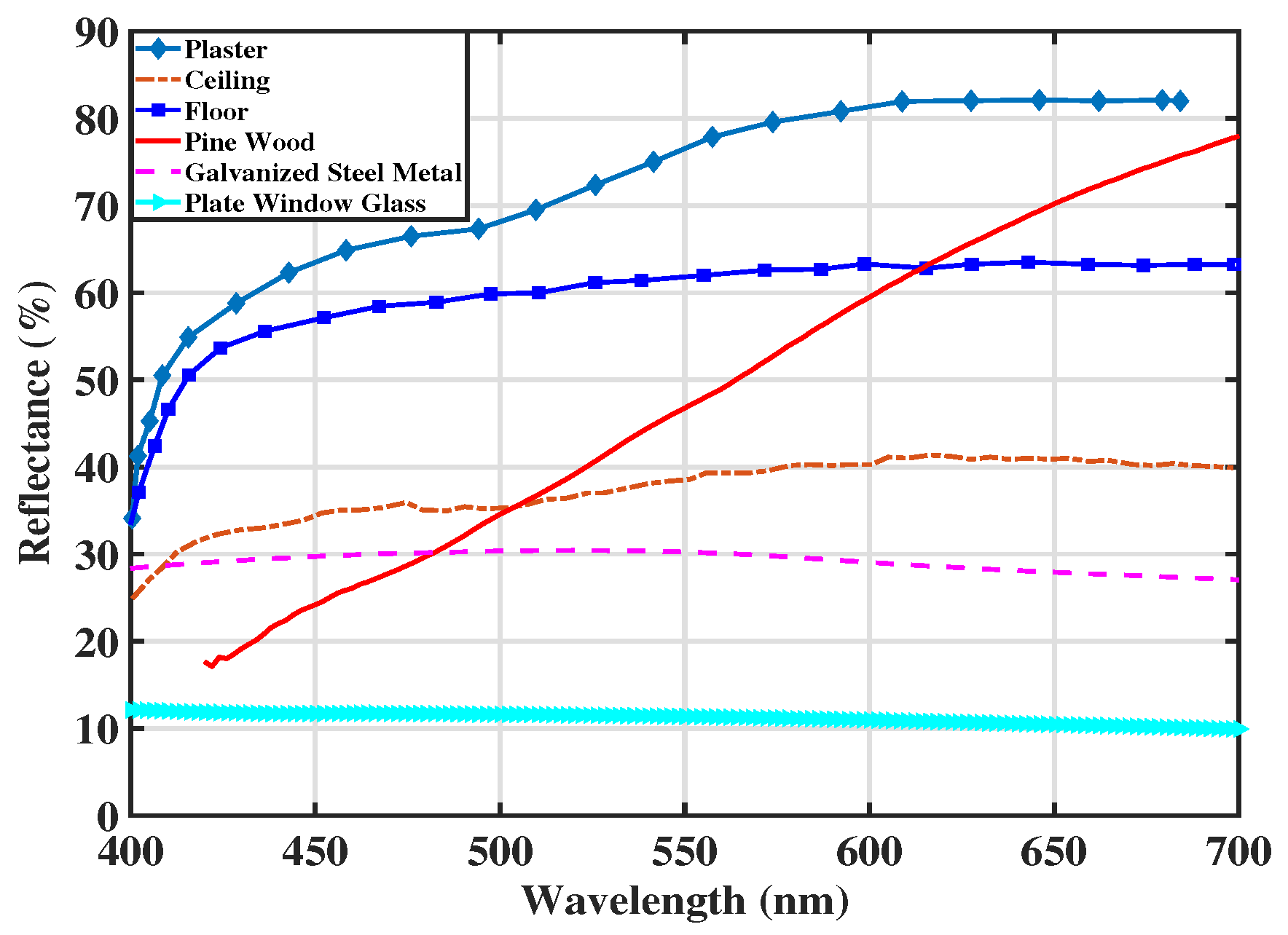
| Material reflectance | Wavelength-dependent | |
| Type of reflections | Specular and diffuse reflections | |
| Coating material | Walls | Plaster |
| Ceiling | Ceiling | |
| Floor | Floor | |
| Table, desks, and doors | Pine Wood | |
| TV screen | Plate Window Glass | |
| TV shelf and electric box | Galvanized Steel Metal | |
| Scatter fraction | TV screen | 0.2 |
| Desks and doors | 0.5 | |
| Other objects | 1 | |
| TX | Model of LED | PAR20 |
| Number of LED | 9 | |
| Optical power of each LED | 2 W | |
| Analysis rays | ||
| Minimum relative ray intensity | ||
| Channel | Length | 3–10.51 m |
| Delay resolution | 0.2 ns | |
| RX | Type of receiver | Detector Polar |
| Radial size | 10 mm |
Publisher’s Note: MDPI stays neutral with regard to jurisdictional claims in published maps and institutional affiliations. |
© 2022 by the authors. Licensee MDPI, Basel, Switzerland. This article is an open access article distributed under the terms and conditions of the Creative Commons Attribution (CC BY) license (https://creativecommons.org/licenses/by/4.0/).
Share and Cite
Liu, B.; Tang, P.; Zhang, J.; Yin, Y.; Liu, G.; Xia, L. Propagation Characteristics Comparisons between mmWave and Visible Light Bands in the Conference Scenario. Photonics 2022, 9, 228. https://doi.org/10.3390/photonics9040228
Liu B, Tang P, Zhang J, Yin Y, Liu G, Xia L. Propagation Characteristics Comparisons between mmWave and Visible Light Bands in the Conference Scenario. Photonics. 2022; 9(4):228. https://doi.org/10.3390/photonics9040228
Chicago/Turabian StyleLiu, Baobao, Pan Tang, Jianhua Zhang, Yue Yin, Guangyi Liu, and Liang Xia. 2022. "Propagation Characteristics Comparisons between mmWave and Visible Light Bands in the Conference Scenario" Photonics 9, no. 4: 228. https://doi.org/10.3390/photonics9040228
APA StyleLiu, B., Tang, P., Zhang, J., Yin, Y., Liu, G., & Xia, L. (2022). Propagation Characteristics Comparisons between mmWave and Visible Light Bands in the Conference Scenario. Photonics, 9(4), 228. https://doi.org/10.3390/photonics9040228